This document is a thesis submitted by Aad Vijn to the Delft University of Technology in partial fulfillment of the requirements for a Master of Science degree in Applied Mathematics. The thesis investigates inverse modeling techniques to predict the magnetic signature of naval ships based on onboard measurements of the magnetic field and an accurate description of the ship's steel geometry. The thesis first derives the relevant forward and inverse problems and discusses the ill-posed nature of the inverse problem. It then presents methods for discretizing and solving the inverse problem, including regularization techniques. The performance of the resulting prediction model is analyzed using both simulated and real measurement data obtained from a measurement campaign on a mock-up model. While initial results are promising, the thesis identifies several


![TNO report S10099 2016 iii/116
Nomenclature
Below one can find a list with acronyms and notations used in this thesis. The list is
ordered by first appearance in this thesis and per chapter.
Symbols used in Chapter 1
E Electromotive force
ΦB Magnetic flux
n Unit normal vector
B Magnetic induction field
H Magnetic field
µ0 Magnetic permeability in vacuum
M Magnetization of some object
· M Divergence of the magnetization [A/m2
]
M4 Mock-up for Magnetic Monitoring Measurements
Symbols used in Chapter 2
D Electric flux intensity [C/m]
ρ Electric charge [C/m3
]
B Magnetic induction field in tesla [T]
E Electric field intensity [V/m]
H Magnetic field intensity [A/m]
J Electric current density [A/m3
]
∂
∂t Time-derivative
× H curl of H
µ0 Magnetic permeability in vacuum
Ω Steel object
ϕ Magnetic scalar potential
σ Magnetic surface charge
n normal vector w.r.t. Ω
t Thickness of Ω
(f) Gradient of f
∂
∂ν Normal derivative
E Set of triangular elements](https://image.slidesharecdn.com/f392f75a-f6d2-48ac-b3d4-ead9525b344d-160228130847/85/Thesis-9-320.jpg)


![TNO report S10099 2016 3/116
the magnetic signature, electric signature and acoustic signatures and above water
ship signatures such as IR and RCS signatures.
In figure (1.3) one can find the Zr.Ms. Van Speijk (F828) multi-purpose frigate. The
Royal Netherlands Navy has the ambition to equip future naval vessels with a so-
called signature monitoring system. This system should visualize the signature of
different influences. To reduce the signatures of a vessel, the signature monitoring
system has to be coupled to some control system that minimizes the signals. Such
a system is then called a signature management system. During a mission the
signature management system should also warn and give advice if the threat level
becomes critical.
With a so-called degaussing system the magnetic field around the naval vessel can be
reduced. By placing large coils in a ship’s hull (in all three directions) the degaussing
system is able to generate a magnetic field. Such a magnetic field is then used to
reduce the magnetic induction field around a vessel. An extensive explanation of
these systems can be found in [15].
The ultimate task is to complete the creation of a closed-loop degaussing system.
This is essentially the connection between the signature monitoring system and the
degaussing system (and thus a crucial module in the signature management system).
By using the magnetic signature from the signature monitoring system the degauss-
ing system can operate optimally.
Figure 1.3: Multi-purpose frigate Zr.Ms. Van Speijk (F828). Source:
http://www.defensie.nl](https://image.slidesharecdn.com/f392f75a-f6d2-48ac-b3d4-ead9525b344d-160228130847/85/Thesis-27-320.jpg)


![6/116 TNO report S10099 2016
1.2 The magnetic naval mine
The following is an excerpt of chapter 3 in [13]. A summary is given of the history of
the naval mine and the mechanics behind the magnetic naval mine. It will become
clear why there is a need of precise magnetic signature computations for future naval
vessels.
1.2.1 The very first naval mine
The naval mine was first invented by David Bushnell during the American Revolu-
tionary War in the eighteenth century. This primitive mine, if one could speak of a
“mine” at all, was in principle a tar covered beer keg filled with gunpowder. The tar
was necessary to make the keg waterproof. the wood lets the kegs float on water.
The detonation was based on a flintlock mechanism that hopefully got triggered when
the beer keg made contact with a ship’s hull. This type of mine is called a contact
mine. These contact mines were obviously unreliable as the trigger mechanism would
not always work properly. Furthermore, the gunpowder could get wet so that the mine
could not work at all. Yet it was a brilliant first step to the modern naval mines. An
illustration of such a typical beer keg mine can be found in figure 1.4.
Figure 1.4: Beer keg mines in the 18th century. [13]
After the American Revolutionary War, further development of contact mines led to
a reliable detonation mechanism based on pressure/touch. The flintlock mechanism
was replaced by the typical pins.
A pin was “made out of a soft lead that covered a glass vile filled with an electrolyte”.
When a pin contacted the ship’s hull, the glass would break and the electrolyte would
flow between two contacts so that a closed circuit was formed. This then led to the
detonation of the mine.](https://image.slidesharecdn.com/f392f75a-f6d2-48ac-b3d4-ead9525b344d-160228130847/85/Thesis-30-320.jpg)
![TNO report S10099 2016 7/116
The contact mines had a spherical shape, with the typical pins on top of the sphere,
and were held in place by an anchor below the water surface in such a way that
the mines were out of sight of the human eye, but in reach of the vessel’s hull. This
type of naval mine was used excessively in the first World War. They were moored
throughout the waters of Europe and the North sea. It appeared to be an effective
device to defend against submarines.
1.2.2 From contact mines to influence mines
After World War I, Germany started the development of mines that are actuated not
by contact, but rather by influence fields from ships, such as magnetic fields and
electric fields. Germany developed a bottom influence mine that lies on the sea floor
and explodes when it detect a ship’s magnetic field by its distortion of the background
field.
In figure 1.5, one can see the typical detonation mechanism. A dip-needle, which
is also used in a simple compass, reacts on the change from the background field
when a ship is nearby, and closes a circuit when the change was significant enough.
This simple idea is rather brilliant. Without any modern technology they were able to
build a sensor that was rather cheap and worked very well. These mines were used
extensively during World War II.
Figure 1.5: Schematic of a dip needle firing circuit in a magnetic bottom mine used in
World War II. [13]
The U.S. took a different approach in the development of a magnetic mine. Their
magnetic mine sensor was not based on a dip-needle but rather on Faraday’s law of
induction. Given a closed circuit C which encloses an open surface S, Faraday’s law
of induction is expressed by the following formula
E = −
dΦB
dt](https://image.slidesharecdn.com/f392f75a-f6d2-48ac-b3d4-ead9525b344d-160228130847/85/Thesis-31-320.jpg)


![TNO report S10099 2016 13/116
2 Model formulation
In this chapter we start with the formulation of two problems that are used in the
construction of our prediction model, namely the forward and inverse formulation.
The forward problem is derived from the Maxwell’s equations and the inverse problem
follows from the forward problem.
After the computation and approximation of solutions of the forward problem we use
these expressions as a start of the formulation of the inverse problem. Together with
the forward formulation we can define the prediction model.
2.1 Maxwell’s Equation
In the late 1800s the knowledge of electric and magnetic fields was summarized by
Maxwell’s equations:
· D = ρ Gauss’ law: electrical fields are produced by
electrical charges
· B = 0 Gauss’ law: there exist no magnetic
monopoles
× E = −∂B
∂t Faraday’s law of induction: changing mag-
netic fields produce electric fields
× H = ∂D
∂t + J Amp`ere’s law: magnetic fields result from
currents and changing electric fields
In these equations E stands for the electric field intensity [V/m] and H stands for
the magnetic field intensity [A/m]. The quantities D and B stand for the electric and
magnetic flux densities respectively. The units of these quantities are [C/m2
] and [T]
respectively. The magnetic flux density may also be called the magnetic induction
field. The electric charge density [coulomb/m3
] is given by ρ and J stands for the
electric current density measured in [A/m2
].
We see that in general the electric and magnetic fields are coupled by the above
equations. We therefore speak of the electromagnetic field. When we assume that
the fields are static, i.e., the fields do not change in time, then the four equations de-
couple into two sets of two equations that describe the electric field and the magnetic
field. Assuming that there are no currents present (J ≡ 0), the static magnetic field is
described by
· B = 0
× H = 0](https://image.slidesharecdn.com/f392f75a-f6d2-48ac-b3d4-ead9525b344d-160228130847/85/Thesis-37-320.jpg)


![TNO report S10099 2016 17/116
2.4 Derivation of the inverse problem
In this section the linear inverse problem is derived. We want to note that in Chapter 3
we give a general overview of inverse theory. For now we give a heuristic idea behind
the inverse problem. From the forward problem description in the previous section we
know that, given some magnetization M of an object Ω, the induced magnetic field
can be computed via formula 2.3.
The integral equation that defines the inverse problem is given in the following formu-
lation: Given the function B : R3
Ω → R3
, determine continuous source functions
f, g and h such that
B(r) = −
µ0t
4π
Ω
r − r
|r − r |3
f(r )dr +
µ0t
4π ∂Ω
r − r
|r − r |3
g(r )dr
+
µ0t
4π
Ω
∂
∂ν
r − r
|r − r |3
h(r )dr := R(f)(r) + S(g)(r) + T(h)(r)
(2.5)
where R, S, T are the corresponding integral operators. The volume of object Ω is a
compact subset of R3
. Here, f and h respresent the magnetic sources in Ω and g
is the magnetic source on the boundary ∂Ω. The vector function B is the magnetic
induction field, generated by these sources.
Therefore the task is, given measurements of the magnetic induction field B, to find
source functions f, g and h such that the generated field by these sources matches
the measurements as accurate as possible.
Unfortunately in the situation we just described, we normally do not have access to
a full description of the magnetic induction field B. However, we can measure the
magnetic induction field by means of magnetic field sensors. We can measure the
field by a finite number of measurements and the more measurement points available,
the more information about B may be known.
To be able to solve the inverse problem, we reduce it to a finite-dimensional one.
For instance this can be done by a so-called expansion method or by approximating
the integrals involved in the inverse formulation by appropriate quadrature rules. This
finite-dimensional formulation allows us to use magnetic field measurements as input
for the inverse problem.
2.4.1 Petrov-Galerkin Expansion Method
In [10, Ch. 3, p. 25-26] the so-called Petrov-Galerkin method is described for inverse
problems defined over intervals. This expansion method can be used (like finite ele-
ment methods) to derive a system of linear equations. Solutions of such systems are
then approximations of solutions of the inverse problem.
In this section we extend the Petrov-Garlerkin method mentioned in [10] to multiple
dimensions and apply this method to our inverse problem.](https://image.slidesharecdn.com/f392f75a-f6d2-48ac-b3d4-ead9525b344d-160228130847/85/Thesis-41-320.jpg)


![20/116 TNO report S10099 2016
Here, the inner product ·, · 2is defined by
f, g 2 =
R3Ω
f(r)g(r)dr
For simplicity the following “inner product” between a function f : R3
Ω → R and
g : R3
Ω → R3
is defined
f, g :=
(f)x, (g)x 2
(f)y, (g)y 2
(f)z, (g)z 2
=
R3Ω
f(r) g(r)dr
Returning to the orthogonality relations, for each ψi equation 2.6 can be expressed
as
ψi, ν − B =
M
j=1
pj ψi, Rϕj +
N
j=1
pj+M ψi, Sϕj +
M
j=1
pj+(M+N) ψi, Tϕj (2.7)
which leads to a system of linear equations
[Af |Ag|Ah]
pf
pg
ph
= b or simply Ap = b (2.8)
where A is a 3K × (M + N + M) matrix, p is a (M + N + M) × 1 vector and b is a
3K × 1 vector. The matrix A is called the field matrix that contains the physics model
involved, and b is called the load vector. For i = 1, 2, . . . , K equation 2.7 leads to
three rows in A and 3 entries in the vector b:
[3 × 1] aij = ψi, Rϕj for j = 1, 2, · · · , M
[3 × 1] aij = ψi, Sϕj for j = M + 1, 2, · · · , M + N
[3 × 1] aij = ψi, Tϕj for j = (M + N) + 1, 2, · · · , 2M + N
[3 × 1] bi = ψi, B
To solve our specific integral equation we choose the following basis functions:
(I) (ϕi)M
i=1 are linear functions on E [three basis functions per internal element e (tri-
angles)]
(II) (ϕi)N
i=1 are linear functions on BE [two basis functions per boundary element be
(line elements)]
(III) (ψi)K
i=1 are vector functions that consist of delta functions defined on R3
Ω:
ψi(r) =
δ(x − xi)
δ(y − yi)
δ(z − zi)
:= δ(r − ri) where ri = (xi, yi, zi)T
is the location of a
measurement.](https://image.slidesharecdn.com/f392f75a-f6d2-48ac-b3d4-ead9525b344d-160228130847/85/Thesis-44-320.jpg)

![22/116 TNO report S10099 2016
Let u1, u2 and u3 denote the three linear basis functions on the standard triangle Tst.
This means that u1 is one in the vertex (0, 0) and zero in the other vertices, u2 is one
in the vertex (1, 0) and zero in the others, and u3 is one in the vertex u(0, 1) and zero
in the others. Each of the ui is of the form ui(r) = ai
0 + ai
1s + ai
2t for i = 1, 2, 3. It is
now the task to determine the coefficients such that the above conditions holds for
i = 1, 2, 3. The ui(r) should be right in their own vertices:
1 0 0
1 1 0
1 0 1
a1
0 a1
1 a1
2
a2
0 a2
1 a2
2
a3
0 a3
1 a3
2
=
1 0 0
0 1 0
0 0 1
The above system is non singular, hence for every internal element e we can compute
the coefficients exactly, leading to
u1(s, t) = 1 − s − t, u2(s, t) = s, u3(s, t) = t, for (s, t) ∈ Tst
These functions can be used to define the basis functions ϕ1, ϕ2 and ϕ3 on the in-
ternal element E (By taking suitable compositions of u with the transformation r).
However, only the basis functions u1,2 and u3 on each triangular element E are re-
quired to compute the entries of the matrix A in equation 2.8. This becomes clear
when we approximate the entries of the matrix A in the next section.
2.4.4 Construction of basis functions ϕi
Suppose that BE denotes a boundary element with vertices v1 and v2. We look for
two linear basis functions ϕ1 and ϕ2 such that
ϕi(vj) = δij, ϕi is linear on be, ϕi ≡ 0 outside be
Similar to the steps we have taken in the previous subsection, we look at basis func-
tions defined on the interval [−1, 1]. Let r : [−1, 1] → be given by
r =
1
2
(v1 + v2) −
1
2
ξ(v2 − v1), ξ ∈ [−1, 1]
See Figure 2.3. The corresponding basis functions u1 and u2 are given by:
u1(ξ) =
1
2
−
1
2
ξ, u2(ξ) =
1
2
+
1
2
ξ, for ξ ∈ [−1, 1]
which satisfies u1(−1) = 1, u1(1) = 0 and u2(−1) = 0, u2(1) = 1.
x
y
z
[ | ]
r
(x1, y1, z1)
(x2, y2, z2)
−1 1ξ
Figure 2.3: Boundary line element transformation.](https://image.slidesharecdn.com/f392f75a-f6d2-48ac-b3d4-ead9525b344d-160228130847/85/Thesis-46-320.jpg)


![TNO report S10099 2016 27/116
we measure the magnetic signature at different positions, hence the rows of matrix A
are independent and therefore our discrete inverse problem is always consistent.
This means that we always encounter non-uniqueness of a solution of our inverse
problem. To resolve this issue, we can enforce extra constraints on the solution that
we seek. An example of such a constraint is given in example 3.3.1.
2.6.2 Different approach
In this chapter, we have derived the forward formulation of the magnetic field of some
steel object Ω, based on magnetization M. Next, based on the forward formulation,
an inverse formulation is derived. The Petrov-Galerkin method is used to reduce the
inverse formulation to a discrete linear inverse problem (based on a predefined mesh
of object Ω).
As explained in the introduction (section 1.3), Chadebec and his colleagues devel-
oped inverse formulations based on finding some magnetization M of the steel ob-
ject. In [26] they state that the magnetic field of some ferromagnetic material can be
calculated via
Hred = −
1
4π
grad
Ω
M ·
r − r
r − r 3
dΩ
where M is the magnetization of the ferromagnetic material Ω. The inverse problem
is finding the magnetization M via
M +
χr
4π
grad
Ω
M ·
r − r
r − r 3
dΩ = χrH0
where H0 is some external background field and χr is the magnetic susceptibility.
We want to emphasize the different approach of our derivation of the inverse prob-
lem, compared to the approaches in [3, 26, 5]. While the above stated formulation
searches for the magnetization, we are actually not interested in the specific magne-
tization M of Ω itself. We only need some description of the magnetic sources f, g
and h, where f is (a discretised version of) · M, h is one of ν · M in Ω and g a
discretised version of n · M on ∂Ω. By this choice we believe that we can achieve
better approximations of the magnetic sources. Furthermore, in our formulation we
always find magnetic sources that come from a physical magnetization, whereas the
formulation of Chadebec and his colleagues may produce magnetizations that are
not physical.](https://image.slidesharecdn.com/f392f75a-f6d2-48ac-b3d4-ead9525b344d-160228130847/85/Thesis-51-320.jpg)


![TNO report S10099 2016 31/116
precisely the opposite of a forward problem. Such problems are called inverse prob-
lems, see figure 3.2.
When considering inverse problems one wants to determine causes for some ob-
served effects or one wants to determine material properties that can not be observed
directly.
Definition 3.2.1 (Inverse problem). Consider the Fredholm integral equation of the first kind
g(s) =
Ω
K(x, s)f(x)dx
where the (smooth) kernel K and the function g are known. The kernel represents the under-
lying (physical) model. The inverse problem consists of computing f given the function g and
kernel K.
Remark: Throughout this thesis we talk about a specific type of inverse prob-
lems, namely the task of approximating the sources that cause some measured
effect. Therefore, if we talk about an inverse problem, we are always referring to
such inverse problems.
Return to the inverse problem. For the one-dimensional unbounded case (where Ω =
R, f = 0 and k = 1) the final temperature distribution u(x, T) at time T is related to
the initial temperature distribution u(x, 0) via [7]
1
2
√
πT
∞
−∞
u(s, 0) exp −
(x − s)2
4T
ds = u(x, T) (3.1)
Such a problem can also be seen as an inverse problem, although in this case we
are not looking for the sources that have caused the final temperature distribution but
rather the initial temperature distribution.
The above equation is a so-called convolution equation with kernel
K(x, s) =
1
2
√
πT
exp −
(x − s)2
4T
One can show that solutions of the above convolution equation are smooth due to the
properties of the kernel k(x, s). This makes the inverse problem very hard to solve as
initial temperature distributions are not a priori smooth (if the initial temperature dis-
tribution u(s, 0) contains some discontinuities, then the smooth kernel resolves these
in the final temperature distribution). The local variations in the initial temperature
distribution cannot be well determined in an inverse problem.
Cause Effect
inverse
problem
Figure 3.2: Inverse Problem](https://image.slidesharecdn.com/f392f75a-f6d2-48ac-b3d4-ead9525b344d-160228130847/85/Thesis-55-320.jpg)
![32/116 TNO report S10099 2016
3.2.1 Smoothing properties of integral equations
The integral equation in its general form defined by
y(s) =
Ω
K(x, s)f(x)dx
has so-called smoothing properties. In the heat equation example, the function u(x, T)
is in general much smoother compared to u(s, 0). This behavior makes it hard to find
the correct solutions of the inverse problem. The smoothing property of these integral
operators is formulated in the following lemma of Riemann-Lebesgue.
Riemann-Lebesgue Lemma. Let K be a square-integrable function on the closed interval
[a, b]2
. Then
y1(s) =
b
a
K(x, s) sin(λx)dx → 0, (for λ → ±∞)
y2(s) =
b
a
K(x, s) cos(λx)dx → 0, (for λ → ±∞)
Proof. A proof of the Riemann-Lebesgue lemma can be found in [8].
We can interpret this lemma1
as follows. As the frequency λ increases, the ampli-
tudes of the functions y1 and y2 decrease. So higher frequencies are being damped
by the kernel K(s, t), hence functions y1 and y2 become smoother by applying this in-
tegral operator with kernel K to function f(t). Notice that the lemma is formulated for
square- integrable functions only on compact intervals of R2
. However, this theorem
can be found in a more general setting.
If we consider the Riemann-Lebesgue lemma for inverse problems, the reverse hap-
pens: we observe that such a kernel K actually amplifies high frequencies and the
higher the frequency, the more the amplification. This leads to large variations in the
solution of the inverse problem. Furthermore, small perturbations in g1 and g2 can
lead to very large perturbations of the source f when the perturbation of g1 and g2
contains a high frequency component.
This smoothing property of the forward problem is a huge problem from a fundamental
point of view . It makes inverse problems significantly more complex and harder to
“solve”.
3.2.2 General formulation
Consider some linear operator T between Hilbert spaces X and Y given by
T : X → Y, x → y := Tx
1. Observe that we can not apply this lemma to our Heat example. But by truncation of the indefinite
integral in equation 3.1 to some definite integral on some closed interval [a, b] we are able to apply the
Riemann-Lebesgue lemma.](https://image.slidesharecdn.com/f392f75a-f6d2-48ac-b3d4-ead9525b344d-160228130847/85/Thesis-56-320.jpg)


![36/116 TNO report S10099 2016
3.4 Generalized inverse
In this section we define the generalized inverse of an operator T ∈ L(X, Y) where
X, Y are Hilbert spaces. We end by proving that the pseudo-inverse of a bounded
linear operator can be used to compute a least-square solution of minimal norm of
the operator equation Tx = y. The theory summarized in this section can be found in
[7], Chapter 2.
3.4.1 Least-squares and best-approximate solutions
First a definition.
Definition 3.4.1. Let T : X → Y be a bounded linear operator between Hilbert spaces X
and Y. Then
(i) x ∈ X is called a least-squares solution of Tx = y if
Tx − y = inf{ Tz − y : z ∈ X}.
(ii) x ∈ X is called the best-approximate solution of Tx = y if
x = inf{ z : z is a least-squares solution of Tx = y}.
The best-approximate solution is thus defined as the least-square solution with mini-
mal norm. Note that, when X is a Hilbert space, the set of all least-squares solutions
is closed, hence the best-approximation is unique. This is a standard result in Hilbert
theory.
Abstract as it may seem, this concept of best-approximated solution has an applied
side. The actual state of a physical system is usually that with the smallest energy. In
many cases, the energy is formulated by a certain norm and so “minimal energy” is
then equivalent to “minimal norm”, hence a best approximation problem.
3.4.2 Restriction of T
Recall that for an operator T : X → Y (not necessarily bounded) the null-space of
T is defined as N(T) = {x ∈ X : Tx = 0} (which is a subset of X). The range (or
image) of T is defined as R(T) = {Tx : x ∈ X} (which is a subset of Y). For any
subspace Z ⊆ X, the restriction of T to Z is defined as
T Z : Z → Y, T Z (z) = T(z)
In the construction of the generalized inverse we need the following lemma.
Lemma 3.4.1. Let T ∈ L(X, Y) be some bounded linear operator and let X, Y be Hilbert
spaces. Then ˜T, the restriction of operator T, given by
˜T := T N (T )⊥ : N(T)⊥
→ R(T)
is an invertible bounded linear operator.](https://image.slidesharecdn.com/f392f75a-f6d2-48ac-b3d4-ead9525b344d-160228130847/85/Thesis-60-320.jpg)


![42/116 TNO report S10099 2016
3.5 Construction of the generalized inverse for finite-dimensional compact
operators
In this section we consider the construction of the generalized inverse of a compact
finite-dimensional operator, i.e. a matrix operator. The construction can be easily ex-
tended to infinite-dimensional compact operators. However, in this thesis we use the
Petrov-Galerkin method to reduce our inverse problem to a finite-dimensional inverse
problem, so we limit ourselves to the finite-dimensional operators.
Let A ∈ Rn×m
be some real-valued n × m matrix. In [24] it is proven that for any
real-valued n × m matrix there exists a singular value decomposition of the form
A = UΣV T
where U and V are orthogonal matrices and Σ is a diagonal matrix containing the
non-zero singular values of A. Let un and vn denote the columns of the orthogonal
matrices U and V , let σn be the singular values of A defined by
Avn = σnun
then the triple (σn, un, vn) is called a singular system and using this system we obtain
Ax =
r
n=1
σn x, vn un, for any vector x ∈ Rm
where r = rank(A), so the matrix A has r nonzero singular values. For AT
, the
adjoint6
of A, we can derive7
in a similar way a singular system. We have
AT
y =
r
n=1
σn y, un vn, for any vector y ∈ Rn
Note that A†
= (AT
A)†
AT
(see previous section) and hence for x†
= A†
y we have
r
n=1
σ2
n x†
, vn vn = AT
Ax†
= (AT
A)(AT
A)†
AT
y = AT
y =
r
n=1
σn y, vn un
We see by comparing the individual components that it holds that
x†
, vn =
1
σn
y, un
Therefore8
the best-approximate solution of Ax = y is given by (see theorem 3.4.3)
x†
= A†
y =
r
n=1
y, un
σn
vn (3.9)
6. For any m × n matrix A, the adjoint AT
of A, is defined through Ax, y = x, AT
y for all
x ∈ Rn
and for all y ∈ Rm
.
7. The prove is based on the fact that the eigenvalues of the matrices AT
A and AAT
are the same.
Using this property the singular value system follows directly by the same derivation.
8. Ax†
= r
n=1
y,un
σn
Avn = r
n=1 y, un un = y.](https://image.slidesharecdn.com/f392f75a-f6d2-48ac-b3d4-ead9525b344d-160228130847/85/Thesis-66-320.jpg)

![44/116 TNO report S10099 2016
Define T : L2([−1, 1]) → L2(C) to be the bounded linear integral operator
(Tf)(x) =
1
−1
x − x
|x − x |3
f(x )dx
where C ⊂ R [−1, 1] is some compact subset. The boundedness of T follows from
theorem 2.13 in [18]. We start by showing that T is a compact operator.
We claim that the kernel of T is square integrable. Indeed, we have the following
estimate of the kernel K(x, x ):
K 2 =
C [−1,1]
|K(x, x )|2
d(x , x)
=
C [−1,1]
1
(x − x )4
d(x , x)
=
1
3 C
1
(x − 1)3
−
1
(x + 1)3
dx
≤
1
3
µ(C) · maxx∈C
1
(x − 1)3
−
1
(x + 1)3
< ∞
Here the volume of C is finite (as it is a compact subset) and the function
x →
1
(x − 1)3
−
1
(x + 1)3
is continuous on the compact set C, so it has a maximum. Hence we have that K ∈
L2(C × [−1, 1]). We conclude that the operator T is compact.
For given g ∈ L2(C) the inverse problem is to find a function f ∈ L2([−1, 1]) such
that Tf = g holds. We claim that the image of T is infinite-dimensional. To this end
assume that f ∈ L2([−1, 1]) and assume without loss of generality that C ⊂ (1, ∞).
This means that
(Tf)(x) =
1
−1
x − x
|x − x |3
f(x )dx , x ∈ C
can be simplified to
(Tf)(x) =
1
−1
1
(x − x )2
f(x )dx , x ∈ C
Let (xi)∞
i=1 be the sequence in [−1, 1] defined by xi = (1/2)i
and define εi = (1/2)i+2
.
For each i define on the interval [−1, 1] the characteristic function
fi(x ) = χ[xi−εi,xi+εi](x )
Clearly each fi belongs to L2
([−1, 1]) and for i = j the support of the functions fi and
fj are disjoint. Furthermore we have
(Tfi)(x) =
xi+εi
xi−εi
1
(xi − x )2
dx =
1
x − (xi + εi)
−
1
x − (xi − εi)](https://image.slidesharecdn.com/f392f75a-f6d2-48ac-b3d4-ead9525b344d-160228130847/85/Thesis-68-320.jpg)


![TNO report S10099 2016 47/116
4 Regularization Methods and Numerical Solvers
We have seen in the previous chapter that our inverse problem is ill-posed, accord-
ing to Hadamard’s definition of well posedness. We proved that the pseudoinverse
is an unbounded operator, and therefore, the third criterion is violated (continuity).
Furthermore, by reducing the inverse problem to a discrete version we have seen
that the discrete inverse problem has infinite many solutions, which means that the
second criterion of Hadamard’s definition is also violated (uniqueness of the solu-
tion). We discussed a solution this by enforcing an extra constraint on the solution, to
make it unique. We postphoned solutions for the discontinuous behavior of solutions
on the data. In this chapter we will answer the question how we can deal with such
ill-posedness.
Considering the noise in measured data and the ill-posed behavior of inverse prob-
lems, solving an inverse problem is (very) complex. Ordinary application of the pseudo-
inverse to obtain a solution simply fails. Reducing an inverse problem to a finite-
dimensional problem (for instance using the Petrov-Galerkin Method in Chapter 2)
leads to solving a discrete inverse problem of the form
Ax = b (4.1)
Such discrete problems inherit the ill-posed properties of the inverse problems: the
condition number of the matrix A becomes very large. The matrix A is then called ill-
conditioned. Solving ill-conditioned problems is hard because solutions become very
sensitive to small perturbations in the right-hand side b. Therefore one has to add
additional information about the solution x in order to produce feasible solutions. This
is called regularization of the solution. Also, the high condition number may make the
use of direct solving methods useless. Hence we need to consider more advanced
solvers that can produce good solutions.
In this chapter we start with answering the question why we need regularization.
Then, we discuss several standard regularization methods that give us insight in the
fundamental ideas behind regularization. We give a brief explanation about the regu-
larization methods. A detailed overview of these methods can be found in [10].
In the second part of this chapter, we recall the basic ideas behind direct solvers
and the iterative methods. We discuss the so-called conjugate gradient least squares
method (abbreviated by CGLS), which is a small extension of the ordinary CG method
to the non-symmetrical case. This method can be used to solve our inverse problem.](https://image.slidesharecdn.com/f392f75a-f6d2-48ac-b3d4-ead9525b344d-160228130847/85/Thesis-71-320.jpg)

![TNO report S10099 2016 49/116
The above result implies that ill-conditioned matrices A produce solutions that are
very sensitive to (small) perturbations e. We expect that in this case the solution x
may be far away from the exact solution xe. This behavior should be avoided for
accurate predictions of the solution. One way of reducing the sensitivity is to add
extra information to our inverse problem about the solution we seek. This way we
regularize the solution as we reduce the “solution space” of our problem, by adding
extra constraints.
Another way of regularizing the problem is to consider a better conditioned system
A x = b (4.2)
that is “near” the original system in the sense that the solutions of (4.2) approximate
the solutions of the original system and such that the solution is less sensitive to
small perturbations. Such methods are called regularization methods. In fact, there
is a close relationship between A and the pseudo inverse A†
of matrix A. Solutions
of system 4.2 are approximations of x†
and the operator (A )†
approximates A†
. A
theoretical approach of regularization methods can be found in [7].
4.2 Standard Regularization methods
We begin with discussing some standard regularization methods as described in the
introduction. The ideas behind these regularization methods can be used later on
to describe the regularizing effects of the CGLS method. As we will see, the CGLS
method is suitable for the application of regularization.
As always consider the following linear system of equations
Ax = b
where A is a rectangular m × n matrix and b is polluted by a noisy term
b = be + e
Denote by xe the exact solution of the system Ax = be and let (U, Σ, V ) be a singular
system for A, i.e., we can decompose A as
A = UΣV T
Let σ1 ≥ σ2 ≥ . . . ≥ σr > 0 denote the singular values of A, ui the left-singular vector
of A and vi the right-singular vectors of A. As described in the previous chapter, we
can solve the linear system using the pseudo-inverse of A to obtain the naive solution
x†
:= A†
(be + e) =
r
i=1
be, ui
σi
vi +
r
i=1
e, ui
σi
vi (4.3)](https://image.slidesharecdn.com/f392f75a-f6d2-48ac-b3d4-ead9525b344d-160228130847/85/Thesis-73-320.jpg)
![50/116 TNO report S10099 2016
where r = rank(A) is the rank of A. Note that a solution of the system Ax = b drifts
away from the exact solution xe in the presence of some noisy term in b. This means
that if the matrix A is ill-conditioned we can see that in 4.3 the second summation
can become very large due to small singular values. So even if e 2 b 2, we can
expect that the solution x†
is far away from the exact solution xe.
The idea behind some standard regularization methods is to reduce the influence of
noise on the best-approximate solution x†
. There are two method that are based on
this principle: the truncated SVD regularization and Tikhonov regularization.
4.3 Truncated SVD
For this moment we assume that e 2 b 2 and consider expression 4.3. Further-
more we assume that matrix A has a large condition number, such that A has both
large and small singular values and that there is a clear distinction between them.
Now for large singular values σi we assume1
that
b, ui
σi
≈
be, ui
σi
while for small singular values we assume that
b, ui
σi
≈
e, ui
σi
Therefore it seems reasonable to only take in account the first few contributions to the
solution in 4.3 that contain the most information about the signal that we seek. We
simply chop off those SVD components that are dominated by the noise, which are
the SVD terms that correspond to small singular values. This leads to the so-called
truncated SVD (also abbreviated as the TSVD) solution xk as the solution obtained
by retaining the first k components of the naive solution 4.3:
xk =
k
i=1
b, ui
σi
vi, for some k ≤ r (4.4)
In this expression parameter k is called the truncation parameter and serves as a
so-called regularization parameter. The parameter should be chosen in such a way
that the noisy terms that are dominating in the naive solution are neglected. The
choice of the truncation parameter depends on the specific problem that is consid-
ered. In [10, Ch. 5.2 - 5.5] a few parameter choice methods are discussed such as
the discrepancy principle, the so-called Generalized Cross Validation (GCV) method
and the choice of the truncation parameter via a so-called NCP analysis (normalized
cumulative periodogram).
1. We assume that the exact data be satisfies the Picard Criterion, that is, the SVD components decay
faster than the singular values. This guarantees that a square-integrable inverse solution exists. See [10,
chapter 3] for a detailed explanation on the Picard Criterion. It follows from the Picard Criterion that the
two approximations of the SVD components holds.](https://image.slidesharecdn.com/f392f75a-f6d2-48ac-b3d4-ead9525b344d-160228130847/85/Thesis-74-320.jpg)


![TNO report S10099 2016 53/116
is important to produce good solutions. Therefore, the problem in a Tikhonov regular-
ization reduces to finding the correct value for λ such that the solution xλ is the most
optimal one, given some good operator L.
4.4.2 L-curve method to find λ
Several techniques are known about finding the best value of λ. One way of finding the
optimal λ is via the so-called “L-curve” method. This method is based on an intuitive
view of regularization. One can prove that the residual norm
ρ(λ) = Axλ − b 2
2
is monotonically increasing in λ and that the norm of the Tikhonov solution
ξ(λ) = Lxλ
2
2
is monotonically decreasing in λ. This specific behavior of the residual norm and the
norm of the solution implies an “optimal” value λ that is known as the corner of the
graph
Γ(λ) =
1
2
log10 ρ(λ),
1
2
log10 ξ(λ)
One can prove that graph has a typical L-shape. The corner of this L-shaped graph
is then the point for which the corresponding λ is presumed to be as the optimal
value of the Tikhonov regularization method. In the corner there is an optimal balance
between minimizing the residual norm and minimizing the length of Lx. In figure 7.7
an example of an L-curve is shown.
In [10], section 4.7, and in [11] one can find a detailed explanation about this method
and other properties of the L-curve. We omit any further explanation of the L-curve
method in this report and refer to [10] and [11].
4.4.3 Writing the minimization in a different form
The Tikhonov problem formulation in 4.6 can be described as a least-squares prob-
lem in x. This is done by first noting that
y
z
2
2
=
y
z
T
y
z
= yT
y + zT
z = y 2
2 + z 2
2
Applying this result to 4.6 leads to the equivalent problem
min
x
A
λL
x −
b
0
2
2
(4.7)
which is a least-squares problem in x. Such a problem can be solved by first consid-
ering the corresponding normal equations given by
A
λL
T
A
λL
x =
A
λL
T
b
0
](https://image.slidesharecdn.com/f392f75a-f6d2-48ac-b3d4-ead9525b344d-160228130847/85/Thesis-77-320.jpg)
![54/116 TNO report S10099 2016
and then use an appropriate solver to find a (least-squares) solution. For numerical
algorithms is it sometimes better to base the computation of Tikhonov solutions on
4.7 rather than on the normal equations. In the last part of this chapter, in section 4.7,
we consider the CGLS method that is able to solve minimization problems like 4.7.
4.4.4 Tikhonov when L = I
An example of the matrix L is when it equals the identity matrix L = I. The Tikhonov
problem takes the form
xλ = arg min
x
Ax − b 2
2 + λ2
x 2
2
which means that we are looking for solutions such that the 2−norm of that solution
is minimal. The Tikhonov problem is then solved by finding a least-squares solution
of the equation
(AT
A + λ2
I)x = AT
b
which can be solved using the pseudo-inverse of AT
A + λ2
I:
xλ = (AT
A + λ2
I)†
AT
b
Let A = UΣV T
be the singular value decomposition of A. Here, we use the compact
form of the SVD. This means that we can choose matrices U, Σ and V in such a way
that Σ is a diagonal matrix. Using that V V T
= I we find that
xλ = (V Σ2
V T
+ λ2
V V T
)†
V ΣUT
b
= V (Σ2
+ λ2
I)†
V T
V ΣUT
b
= V (Σ2
+ λ2
I)†
ΣUT
b
= V (Σ2
+ λ2
I)−1
ΣUT
b
Here, we have used that for an invertible diagonal matrix the pseudo-inverse is equal
to the inverse matrix. The above expression for xλ can be expressed in terms of
singular values and singular vectors. We obtain the following neat expression for xλ:
xλ =
n
i=1
σ2
i
σ2
i + λ2
uT
i b
σi
vi (4.8)
Observe how the regularization parameter λ influences the regularized solution xλ.
Define
ϕ
[λ]
i =
σ2
i
σ2
i + λ2
≈
1 σi λ
σ2
i
λ2 σi λ
where ϕ
[λ]
i are the so-called filter factors (compare with equation 4.4). For singular
values that are much larger than λ, the corresponding filter factors are close to 1, so
the associated singular value components are not changed a lot, while for singular](https://image.slidesharecdn.com/f392f75a-f6d2-48ac-b3d4-ead9525b344d-160228130847/85/Thesis-78-320.jpg)


![58/116 TNO report S10099 2016
The characteristic polynomial is given by
pA(λ) = det(A − λIn) = det
1 − λ 2
3 4 − λ
= λ2
− 5λ − 2
Now define p(X) = X2
− 5X − 2I2, then one can simply verify that p(A) = 0.
A direct result from the Cayley-Hamilton theorem is that for any invertible matrix A,
the matrix satisfies the following identity:
p(A) = An
+ cn−1An−1
+ · · · + c1A + (−1)n
det(A)In = 0
This leads to the following expression for the inverse A−1
:
A−1
=
(−1)n−1
det A
(An−1
+ cn−1An−2
+ · · · + c1In)
Thus, for any invertible matrix A, its inverse can be expressed into terms of powers
of A (where In = A0
), or
A−1
∈ span(I, A, A2
, . . . , An−1
)
Consider for now the system Ax = b where A is invertible. Due to the above ob-
servations, the Cayley-Hamilton theorem implies that the solution x∗
= A−1
b can be
written as
x∗
= A−1
b =
(−1)n−1
det A
(An−1
+ cn−1An−2
+ · · · + c1In)b
=
(−1)n−1
det A
(An−1
b + cn−1An−2
b + · · · + c1b)
which means that x∗
∈ span(b, Ab, A2
b, . . . , An−1
b). This is the starting point for
Krylov-subspace iterative methods. We define the k-th Krylov subspace Kk(A, b) as-
sociated to A and b to be the subspace spanned by the product of the first k − 1
powers of A and b:
Kk(A, b) = span(b, Ab, . . . , Ak−1
b)
Observe that x∗
∈ Kn(A, b) and for natural numbers p ≤ q that Kp(A, b) ⊆ Kq(A, b).
Krylov-subspace iterative methods are iterative methods that seek the k-th approx-
imation of the solution in the Krylov subspace Kk(A, b) of order k. Because of the
nested behavior of the Krylov subspaces each iterate is a better approximation of the
solution.
One of the first Krylov-subspace methods is the so-called Conjugate Gradient Method
(CG method). Originally this method was formulated for symmetric positive definite
matrices, but later the method was extended to a larger class of matrices. A nice
feature of the CG method is that it only requires one matrix-vector product for each
iteration, and the memory allocation is independent of the number of iterations. This
makes the method a compact solver to implement. A detailed explanation on this
method can be found in [25, Ch. 6].](https://image.slidesharecdn.com/f392f75a-f6d2-48ac-b3d4-ead9525b344d-160228130847/85/Thesis-82-320.jpg)


![TNO report S10099 2016 63/116
4.7.7 Properties of xk and dk
Recall that each iterate in the CGLS method solves the minization problem and that
Kk(AT
A, b) ⊆ Kk+1(AT
A, b). This implies that the discrepancies dk form a non-
increasing sequence
dk+1 ≤ dk
as we minimize the functional in 4.7.7 over a “larger” space.
With some extra effort (using the orthogonality properties of the search directions),
the norms of the solutions form a non-decreasing sequence:
xk+1 ≥ xk
A proof of this property is found in [12, Section 4].
4.7.8 The CGLS method algorithm
The CGLS method algorithm is summarized as follows. For simplicity we set the initial
guess x0 = 0. The algorithm does not contain a stopping criterion, though it is easy
to built in such a criterion in the algorithm.
Algorithm 1 The CGLS Algorithm: given the right hand side b and matrix A
Initialize:
x0 = 0;
d0 = b − Ax0;
r0 = AT d0;
p0 = r0;
y0 = Ap0;
for k = 1, 2, . . . until stopping criterion is satisfied
α =
rk−1
2
2
yk−1
2
2
;
xk = xk−1 + αpk−1;
dk = dk−1 − αyk−1;
rk = AT dk;
β =
rk
2
2
rk−1
2
2
;
pk = rk + βpk−1;
yk = Apk;
end](https://image.slidesharecdn.com/f392f75a-f6d2-48ac-b3d4-ead9525b344d-160228130847/85/Thesis-87-320.jpg)
![64/116 TNO report S10099 2016
4.8 Regularization properties of the CGLS method
Facing ill-posed linear inverse problems of the form
Ax = b + e
we know that the matrix A is ill-conditioned. This means that the condition number
of A is large. (In general, condition numbers of the order of 105
start becoming of
concern.) This is caused by the tiny singular values of matrix A.
When using iterative methods for solving such ill-conditioned linear systems, a semi-
convergence behavior can often be observed. Semi-convergence means that at first
the iterates tend to converge to some meaningful solution, but as the iterations pro-
ceed, they begin the diverge. The divergence can be explained by the noisy term in
the right-hand side of the linear system in combination with the singular values of A.
At some point in the iteration the noise becomes more and more amplified and the
iterates start to diverge from the (least-squares) solution of the system.
The amplification is due to the growing Krylov subspaces. In [10, Ch 6.3.3] Hansen
explains that when we use the CGLS method, after each iteration the Krylov sub-
spaces becomes larger as we are searching for a solution in more search directions.
For the first iterations the CGLS method aims at reducing the discrepancy
dk = b − Axk
in the singular direction associated with the larger singular values. On later iterations
the discrepancy is reduced in the singular directions that are associated with the
smaller singular values. The small singular values begin to spoil the iterates. Hence
we conclude that the CGLS method starts with focusing on the most significant com-
ponents of the SVD expression (the components that contain the most information
about the solution that we seek). In [2], Example 4.6, this behavior is also illustrated.
Therefore, we need to capture the solution in time, before the amplified noise takes
over. This can be done by truncating the iteration in time before the semi-convergence
behavior kicks in. By equipping the iterative method with a stopping rule effective at
filtering the amplified noise from the computed solution, we can make the problem
less sensitive to perturbations in the data. This process of regularizing by a stopping
rule is called regularization by truncated iteration. The idea behind regularization by
truncated iteration is similar to the truncated SVD expression. When we apply the
truncated SVD method, we also try to separate the noise from the solution by trun-
cating the SVD expression, taking only in account the most significant components.
More details on the regularizing effects of the CGLS method can be found in an article
by A. van der Sluis and H.A. van der Horst [23, Section 6].
When the iterative method stops too early, the solution becomes oversmoothed by the
iterative method, while the solution becomes undersmoothed if the iterative method](https://image.slidesharecdn.com/f392f75a-f6d2-48ac-b3d4-ead9525b344d-160228130847/85/Thesis-88-320.jpg)
![TNO report S10099 2016 65/116
does not stop in time. Recall that
dk+1 ≤ dk , xk+1 ≥ xk
where dk is the discrepancy of the k-th iterate. A solution of the system
Ax = b
solved by the CGLS method should be a good fit of the data, while x should not be
large. The above observation suggests that there is an iterate k for which the balance
between a good fit of the data and the length of the solution vector is optimal. This
observation leads to the so-called L-curve for the CGLS method. An example of such
a typical L-curve that we encounter in our inverse problem is shown in figure 4.1. We
omit the explanation of this method and refer to [19]. As discussed in the L-curve
method for Tikhonov regularization, the optimal point on the L-curve of the CGLS
method is the corner with the largest curvature of the graph described by
Γ = log10 dk
2
, log10 xk
2
) , where k = 1, 2, . . .
We will use this criterion when solving our inverse problem with the CGLS method to
find the best approximation to the linear inverse problem.
We want to emphasize that this criterion is not a stopping criterion. In order to have
a clear view on the shape of the graph Γ, we need to do a large number of iterations
to construct Γ. Therefore, this approach does not really seem to be a time efficient
one, but we believe that the solutions found via the L-curve criterion lead to the best
approximations. This idea is tested in Chapter 6.
Figure 4.1: Typical L-curve that we encounter in our discrete inverse problem.](https://image.slidesharecdn.com/f392f75a-f6d2-48ac-b3d4-ead9525b344d-160228130847/85/Thesis-89-320.jpg)


![72/116 TNO report S10099 2016
between two domains 1 and 2, where n2 is the normal vector on domain 2 that is
pointing outwards.
Given an magnetization M of the ferromagnetic object Ω, it is easy to compute the
magnetic field with COMSOL by a so-called finite-element package that is built into
COMSOL. The Galerkin weighted residual method is implemented in COMSOL and can
be used to transform the system of PDE (domain equations plus boundary conditions)
into a large system of linear equations. The idea behind this method is to expand the
potential on a meshed object:
Vm =
n
i=1
WiVi
where Wi are so-called predefined weight functions. See for an explanation on this
approach [3].
It is also possible in COMSOL to compute reduced magnetic fields that are induced
by some present background field. This can be done by solving the problem with a
finite-element method. Again, the system of PDE is transformed into a large system
of linear equations but due to the complexity of this linear system, all kinds of difficul-
ties such as numerical stability and the lack of memory in the solver are introduced.
Therefore extra assumptions are required to reduce the complexity of the problem.
A well known method implemented in COMSOL is the so-called magnetic shielding
condition.
Especially for geometries consisting of thin steel plates, the magnetic shielding method
is a way of adding extra boundary conditions to the problem in order to reduce the
three-dimensional object to a two-dimensional surface. This is based on the follow-
ing two assumptions. The first assumption is that the thickness of the steel plates is
very small and (for the sake of simplicity) the thickness is constant over the plate.
Furthermore, we assume that the magnetization is tangential to the plate, so that
everything “happens” along the surface of a plate. This means that when we decom-
pose the magnetization M into a tangential component M (along the surface) and a
component M⊥
perpendicular to the surface, we have that M⊥
≡ 0.
In [3] and [17] a derivation can be found of the magnetic shielding conditions. The
magnetic shielding conditions are given by
n · (B1 − B2) = − t · (µ0µrt tVm), over the surface ∂Ω
Here, µr is the relative magnetic permeability of the medium and t is the plate thick-
ness. The operator t represents a tangential gradient along the surface. After ap-
plying the Galerkin weighted residual method these conditions transform into linear
equations.
It remains to define proper boundary conditions on the boundary ∂S of the computa-
tion space. These conditions are required in order to have a unique solution and to](https://image.slidesharecdn.com/f392f75a-f6d2-48ac-b3d4-ead9525b344d-160228130847/85/Thesis-96-320.jpg)


![TNO report S10099 2016 79/116
6.2 Simulation: uniform background field along the ux-direction
Let Bb be the static uniform back ground field given by
Bb = 50 · 10−6
ux [T] (6.1)
We compute the magnetic signature of the M4 in COMSOL. We construct a data set of
the magnetic signature that consists of 176 possible sensor positions on-board of the
M4 and construct a data set of the magnetic signature that consists of values at one
meter below the M4 in an array of reference points. The results (the two data sets)
are then exported as plain text files and are converted into matrices in MATLAB.
In Appendix A the results of these CIFV routines can be found. The results based on
176 measurements inside the M4 for four different methods and several meshes of
the M4. In the second table the results are of the use of Tikhonov regularization in
the SVD method. The regularization parameter is chosen with the “L-curve” principle.
Furthermore we investigated the stability of the usage of a QR decomposition. The
iterative CGLS method is applied to the system with a total of 528 iterations (the rank
of A). Due to bad results we have skipped some of the computations of the SVD and
QR method.
6.2.1 Results of CIFV routines
This section presents some results of the application of the prediction model to the
COMSOL input. We consider the magnetic signature of the M4 in a local background
field described in equation 6.1. Therefore, we expect that the induced magnetisation
of the M4 is orientated in the same direction.
A good performance of the prediction model is observed in the case that we mesh the
M4 by mesh IV and using the CGLS method to solve the inverse problem. Here, we
used the L-curve criterion as as stopping criterion for the CGLS method. The L-curve
in this particular case is found in figure 6.5. We see that the optimal solution is found
at k = 137.
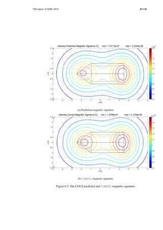
The prediction of the magnetic signature is quite good in this case. We have that the
relative error τ at one meter below the M4 satisfies
0.004 ≤ τ ≤ 0.074
and that the absolute error of the predicted signature satisfies
4.5nT ≤ ε ≤ 117nT,
so the absolute error is maximal 117nT. The relative error and absolute errors at one
meter below the M4 are shown in figure 6.2. The predicted signature and COMSOL
signature are shown in figure 6.3. Observe that the shape of the intensity of the](https://image.slidesharecdn.com/f392f75a-f6d2-48ac-b3d4-ead9525b344d-160228130847/85/Thesis-103-320.jpg)


![TNO report S10099 2016 89/116
6.4.1 Changing the prediction model
In our forward problem formulation, the potential that solves Poissons problem is built
out of single layer potentials and a double layer potential. This potential leads to the
following description of the magnetic induction field outside the mock-up that was
given by (eq 2.3)
B(r) = −
µ0t
4π
Ω
r − r
|r − r |3
· M(r )dr +
µ0t
4π ∂Ω
r − r
|r − r |3
n (r ) · M(r )dr
+
µ0t
4π
Ω
∂
∂ν
r − r
|r − r |3
n (r ) · M(r )dr (6.3)
where the third integral corresponds to the double layer potential. Now for our mock-
up it holds that the thickness of the steel is relatively small to the other dimensions of
the mock-up. Therefore we argue that the contribution of this double layer component
can be neglected in the prediction model. The magnetic field in the forward problem
is then described by
B(r) = −
µ0t
4π
Ω
r − r
|r − r |3
· M(r )dr +
µ0t
4π ∂Ω
r − r
|r − r |3
n (r ) · M(r )dr
(6.4)
and the inverse problem is the task of finding magnetic sources f and g that fit the
measurements.
6.4.2 Results neglecting the double layer component
We investigate the performance of the prediction model in the absence of the double
layer component. In Table 6.2 the errors of the prediction can be found. Observe
that when we neglect the double layer component, the performance of the prediction
model increases significantly. In particular, for mesh V we see that the prediction is
more or less perfect, with an absolute error of maximal 34nT. In figure 7.9c the results
in this case are shown.
With double layer component Without double layer component
Mesh εmax [nT] τmin τmax εmax [nT] τmin τmax
Solver:CGLS
I 208 0.004 0.097 106 0.018 0.055
II 176 0.012 0.103 74 0.001 0.042
III 152 0.009 0.093 65 0.002 0.042
IV 71 0.003 0.054 71 0.003 0.054
V 126 0.007 0.088 34 0.005 0.042
VI 150 0.007 0.087 158 0.021 0.081
Table 6.2: Simulation errors based on 176 measurements inside the M4. We compare
the simulation errors of the prediction with and without the double layer component.](https://image.slidesharecdn.com/f392f75a-f6d2-48ac-b3d4-ead9525b344d-160228130847/85/Thesis-113-320.jpg)


![92/116 TNO report S10099 2016
6.5 Noisy Measurements and the use of Regularization
In the previous sections we analyzed the prediction model’s performance. We have
seen the performance of the prediction model for different meshes and solvers, and
we saw that the CGLS method produced the best inverse solutions. However, in the
simulations we did not considered any noisy measurements (besides any numerical
rounding errors in COMSOL, but these are small). In this section we consider noisy
measurements and investigate to what extent the regularizing behavior of the CGLS
can deal with this noise.
6.5.1 Modeling of noise
Suppose that our discrete inverse problem is of the form
Ap = b + e
where we introduce a noise term δ in the vector b. We model the noisy δ as Gaussian
noise with mean zero. For each measurement vector x ∈ R3
at some sensor position
we have that
δ ∼ N(0, σ2
I3)
with probability density
πδ(x) =
1
(2π)
3
2 σ3
exp −
1
2σ2
x 2
The covariance matrix Σ = σ2
I3 indicates that the entries δi of noise vector δ are
independent. Noise that is modeled in this manner is called white Gaussian noise.
For K sensor positions the noise vectors can be concatenated to a vector e, the
noise vector that appears in the discrete inverse problem.
When we measure the magnetic field inside the M4 using a magnetic flux-gate sen-
sor, experience learned that the measurement can deviate a couple of hundreds of
nanotesla. More specifically,
Bexact(r) − Bmeasured(r) 2 ≤ 300nT, for each measurement r
Therefore, a reasonable value for σ is
3σ =
1
3
√
3 · 300 · 10−9
T
so that 99% of the mass below the probability density lies within the interval [−3σ, 3σ].
This means that the noise in each measurement most likely varies between 0nT and
300nT. Hence, the model for the noise in each sensor position is given by
δ ∼ N(0, σ2
I3), σ =
1
9
√
3 · 300 · 10−9
(6.5)](https://image.slidesharecdn.com/f392f75a-f6d2-48ac-b3d4-ead9525b344d-160228130847/85/Thesis-116-320.jpg)


![TNO report S10099 2016 99/116
7.1.1.8 Permstate II
With the new perm state, we execute another set of measurements. Instead of con-
sidering the background fields in the first run, we looked at another set of background
fields: (1) zero field, (2) the local earth magnetic field at B¨unsdorf, (3) a uniform back-
ground field in the z-direction and (4) a uniform background field in the x-direction.
The earth magnetic field at the facility in B¨unsdorf is approximately
Bx = 17575nT, By = 690nT, Bz = 46500nT
These values are found using a numerical model of the “National Centers for Environ-
mental Information” [22]. B¨unsdorf is at latitude 54.4◦
North and longitude 9.730542◦
East.
7.1.1.9 Schedule
In table 7.1 we give an overview of the plan for the measurement campaign. Observe
that by zero field, we mean that the Helmholtz coils generate a magnetic field that
cancels out the earth magnetic field.](https://image.slidesharecdn.com/f392f75a-f6d2-48ac-b3d4-ead9525b344d-160228130847/85/Thesis-123-320.jpg)


![TNO report S10099 2016 109/116
8 Conclusion and Further Research
8.1 Results
In the introduction we defined five research goals:
• Determine a correct formulation of this prediction model.
• Analyze the inverse problem and study regularization methods.
• Use simulated data to investigate whether the model can predict accurately.
• Analyze the influence of noise in the measurement data with respect to the solu-
tions of the inverse problem.
• Apply the prediction model to real on-board measurement data.
In chapters 2-4 we have covered the first two research goals. We have determined
a formulation of a prediction model, under suitable assumptions. Furthermore, its
behavior and regularization methods have been studied. The correctness of the for-
mulation seems to be justified by numerical experiments. We are confident that the
proposed prediction model is able to predict the magnetic signature, based on on-
board measurements of the magnetic field.
8.1.1 Performance of the prediction model
In Chapter 7 we have investigated the performance and behavior of the prediction
model, based on simulations in COMSOL. We have seen that the prediction model per-
forms well with these simulations of a background field. For the uniform background
field Bb = 50 · 10−6
uxT we have seen that the prediction model (in the absence of
noisy measurements) performs very good: the best performance was observed in the
numerical test where we neglected the double layer component in the forward and
inverse problem formulation. A maximum absolute error εmax of around 34nT and a
relative error in the range of [0.005, 0.042] was obtained. Relatively, this means that
the predicted signature is maximally 4 percent off. (In practice, a maximal percentage
of 10 percent is acceptable.) However, many on-board measurements (176 measure-
ments) are required to achieve these results.
8.1.2 Reducing the influence of noise in measurements on performance
We also investigated the effect of regularization when we used noisy measurements
in the prediction model. We defined a simple noise model and added this noise to the
on-board measurements of the signature. The noise vector e was modeled as White
Gaussian noise, where each of the entries ei were independently normally distributed.
As a reasonable value for σ we took the value
σ =
1
9
√
3 · 300 · 10−9
T](https://image.slidesharecdn.com/f392f75a-f6d2-48ac-b3d4-ead9525b344d-160228130847/85/Thesis-133-320.jpg)


![112/116 TNO report S10099 2016
the solution (should) satisfy can be used in formulating an a-priori distribution of X.
Notice the similarity between these a-priori distributions and the notion of Tikhonov
regularization. In fact, one can show that, in this Bayesian statistical framework, these
two notions are the same.
Lastly, the notion of Bayesian learning sounds promising as an enhancement of the
prediction model. For an introduction to Bayesian statistics, we refer to [2].
8.2.2 Advanced regularization methods
As already noted, the notion of prior densities in the Bayesian framework is closely
related to Tikhonov regularization. In this project we look at Tikhonov regularization
to regularize solutions of the inverse problem. As we have shown in section 4.4, a
Tikhonov regularized solution solves the minimization problem
xλ = arg min{ Ax − b 2
2 + λ2
x 2
}
where the parameter λ is chosen in such a way that there is a nice balance between
minimizing the residual r = Ax − b 2
and the norm of the vector x 2
. We also
discussed that the general form of Tikhonov regularization is given by
xλ = arg min{ Ax − b 2
2 + λ2
Lx 2
}
where L is a matrix that contains a-priori information about the inverse solutions. In
this project we took L = I, indicating that we try to limit the norm of the inverse
solutions that we seek. However, by using more advanced information about the so-
lutions, we may improve the performance of the prediction model. For instance, one
could impose a smoothnes conditions on the inverse solution. Imposing the existence
of a first order derivative can be described by the derivative operator
L1 =
−1 1
...
...
−1 1
and a second order derivative is described by
L1 =
1 −2 1
...
...
...
1 −2 1
Besides smoothness conditions one could think of other properties that the inverse
solutions should satisfy. The absence of any magnetic monopoles, which is formu-
lated in Gauss’ law ( · B = 0) leads to the observation that, when we sum up all
magnetic sources, the net charge should vanish. For the magnetic source solutions
f, g and h this implies that
Ω
f(r )dr +
Ω
h(r )dr +
∂Ω
g(r )dr = 0](https://image.slidesharecdn.com/f392f75a-f6d2-48ac-b3d4-ead9525b344d-160228130847/85/Thesis-136-320.jpg)


![TNO report S10099 2016 115/116
Bibliography
[1] L. Baratchart, D.P. Hardin, et al. Characterizing kernels of operators related
to thin-plate magnetizations via generalizations of hodge decompositions. IOP-
SCIENCE Publishing, 2013.
[2] Daniela Calvetti and Erkki Somersalo. Introduction to Bayesian Scientific Com-
puting. Springer, 2007.
[3] Olivier Chadebec, Jean-Louis Coulomb, et al. Modeling of static magnetic
anomaly created by iron plates. IEEE Transactions On Magnetics, 36(4), 2000.
[4] Olivier Chadebec, Jean-Louis Coulomb, et al. How to well pose a magnetization
identification problem. IEEE Transactions On Magnetics, 39(3), 2002.
[5] Olivier Chadebec, Jean-Louis Coulomb, et al. Recent improvements for solv-
ing inverse magnetostatic problem applied to thin shells. IEEE Transactions On
Magnetics, 38(2), 2002.
[6] D.A. Dunavant. High degree efficient symmetrical gaussian quadrature rules for
the triangle. Internation Journal for Numerical Methods in Engineering, 21, 1985.
[7] H. Engl, M. Hanke, and A. Neubauer. Regularization of Inverse Problems. Kluwer
Academic Publishers, 2000.
[8] R. Goldberg. Methods of Real Analysis. Wiley, 1976.
[9] D.J. Griffiths. Introduction to Electrodynamics. Pearson Education, 2007.
[10] Per Christian Hansen. Discrete Inverse Problems. SIAM, 2010.
[11] Per H. Hansen and Dianne P. O’Leary. The use of the L-curve in the regulariza-
tion of discrete ill-posed problems. SIAM Journal on Scientific Computing, 14(6),
1993.
[12] Magnus R. Hestenes and Eduard Stiefel. Methods of conjugate gradients for
solving linear systems. Journal of Research of the National Bureau of Standards,
49(6), 1952.
[13] John Holmes. Exploitation of a Ship’s Magnetic Field Signatures. Morgan &
Claypool, 2008.
[14] John Holmes. Modeling of Ship’s Ferromagnetic Signatures. Morgan & Claypool,
2008.
[15] John Holmes. Reduction of a Ship’s Ferromagnetic Signatures. Morgan & Clay-
pool, 2008.
[16] John David Jackson. Classical Electrodynamics. Wiley, 1999.
[17] L. Kr¨ahenb¨uhl and D. Muller. Thin layers in electrical engineering. example of
shell models in analysing eddy-currents by boundary and finite element methods.
IEEE Transactions on magnetics, 29(2), 1993.
[18] Rainer Kress. Linear Integral Equations. Springer Text, 2010.](https://image.slidesharecdn.com/f392f75a-f6d2-48ac-b3d4-ead9525b344d-160228130847/85/Thesis-139-320.jpg)
![116/116 TNO report S10099 2016
[19] G. Landi. A discrete l-curve for the regularization of ill-posed inverse problems.
A discrete L-curve for the regularization of ill-posed inverse problems.
[20] David C. Lay. Linear Algebra and its applications. Pearson, 4th edition edition,
2010.
[21] E.S.A.M. Lepelaars and D.J. Bekers. Static magnetic signature monitoring, rim-
passe 2011 data analysis and development of a phenomenological model for
cfav quest. Technical report, TNO, 2013.
[22] NOAA. Numerical model for earth’s magnetic field. http://www.ngdc.noaa.
gov/geomag-web/#igrfwmm, June 2009.
[23] A. van der Sluis and H.A. van der Vorst. Sirt- and cg-type methods for the iterative
solution of sparse linear least-squares problems. Elsevier Science Publishing Co,
1990.
[24] A.R.P.J. Vijn. Simplified magnetic signature monitoring. Technical report, TNO,
2015.
[25] C. Vuik and D.J.P. Lahaye. Scientific computing. University Lecture, 2013.
[26] Y. Vuillermet, Olivier Chadebec, et al. Scalar potential formulation and inverse
problem applied to thing magnetic shees. IEEE Transactions On Magnetics,
44(6), 2008.](https://image.slidesharecdn.com/f392f75a-f6d2-48ac-b3d4-ead9525b344d-160228130847/85/Thesis-140-320.jpg)

![Appendix A 2/-116 - TNO report S10099 2016
Mesh εmax [nT] τmin τmax
Solver:SVD
I 7408 0.170 5.407
II 8246 0.510 8.340
III - - -
IV - - -
V - - -
VI - - -
Mesh εmax [nT] τmin τmax
Solver:SVD+Tikh.
I 232 0.005 0.108
II 162 0.013 0.114
III 173 0.007 0.091
IV 88 0.004 0.082
V 124 0.007 0.088
VI 161 0.024 0.106
Mesh εmax [nT] τmin τmax
Solver:QR
I 7397 0.169 5.376
II 8159 0.540 8.290
III - - -
IV - - -
V - - -
VI - - -
Mesh εmax [nT] τmin τmax
Solver:CGLS
I 208 0.004 0.097
II 176 0.012 0.103
III 152 0.009 0.093
IV 71 0.003 0.054
V 126 0.007 0.088
VI 150 0.007 0.087
Table A.1: Results based on 176 measurements inside the M4 for four different meth-
ods. The iterative method CGLS and the application of Tikhonov Regularization in
the SVD solver both lead to good predictions of the magnetic signature for this sensor
configuration.
-](https://image.slidesharecdn.com/f392f75a-f6d2-48ac-b3d4-ead9525b344d-160228130847/85/Thesis-142-320.jpg)


![- TNO report S10099 2016 Appendix C 1/-122
C Double layer potential
In this appendix we discuss a classical result in the field of potential theory. For steel
object we assume that the magnetization is tangential to the surface of the object.
This assumptions works fine when solving the “forward problem” for steel thin shells,
i.e., given some background field Hb determine the reduced magnetic field caused by
the induced magnetization in S. This assumption can be found in many engineering
applications and is called magnetic shielding.
However, in reality a magnetization of a steel thin shell is not entirely tangential to the
shell even though the thickness of the shell is small; there exists some orthogonal
component M⊥
:= M · n (where n ) is the normal vector to the surface S. This
component also induces a potential that is called a double layer potential.
From potential theory we can derive an expression that can describe these contribu-
tions in terms of a scalar magnetic source density distribution on the surface of the
thin shell. This is done in the first section of this appendix. Then, we apply a Sym-
metric Gaussian Quadrature rule to derive an expression of the magnetic induction
field caused by this double layer potential. We end with a physical interpretation of
the double layer potential.
C.1 Further derivation of the potential expression of the Poisson problem
As described in Chapter 4 the forward problem consists of solving Poisson’s problem
∆ϕ = · M
where ·M can be interpret as the source of the potential ϕ. Let us consider for now
the Poisson problem for some single steel plate Ω with dimensions l, w and t (where
t is relatively small compared to the length and width of the plate) and let M be some
magnetization of Ω. We place the steel plate in such a way that the centroid of the
plate coincide with the origin of the (x, y, z)−system, where z is pointing upwards.
The analytical solution of this problem can be formulated in terms of a fundamental
solution ([16], page 176-177):
ϕ(r) =
−1
4π
Ω
1
|r − r |
· M(r )dr
(1a)
+
1
4π
∂Ω
1
|r − r |
n · M(r )dr
(1b)
(1)
Here, the normal vector n is pointing outwards, (1a) is the potential caused by the
divergence of M in the interior of the plate that represents magnetic anomalies in the
-](https://image.slidesharecdn.com/f392f75a-f6d2-48ac-b3d4-ead9525b344d-160228130847/85/Thesis-147-320.jpg)
![Appendix C 2/-122 - TNO report S10099 2016
plate. The second term (1b) is the effective magnetic surface charge σM = n · M
at the surface of the plate. This surface charge exists as the magnetization suddenly
vanishes outside the plate (note that the magnetization is zero outside the plate!).
Therefore, there is a discontinuity of the magnetization at the surface of the plate,
that creates σM.
We take a look at (1b). Define the sets (see figure C.1)
∂Ω1 = v ∈ Ω : [v]z = ±
t
2
= ∂Ω+
1 ∪ ∂Ω−
1
∂Ω2 = v ∈ Ω : [v]x = ±
l
2
∨ [v]y = ±
w
2
By splitting the boundary of the plate into the two regions ∂Ω1 and ∂Ω2 we write (1b)
as
(1b) :=
1
4π
∂Ω1
1
|r − r |
n · M(r )dr
(2a)
+
1
4π
∂Ω2
1
|r − r |
n · M(r )dr
(2b)
(2)
Let Ω be the two-dimensional projection of Ω onto the (x, y)-plane (a rectangular
domain in the (x, y)-plane of dimensions l and w as seen in figure C.2) with a one-
dimensional boundary ∂Ω . We assume that the magnetization is uniform in t. Then
(2b) is simplified to
(2b) :=
t
4π ∂Ω
1
|r − r |
n · M(r )dr
On the boundary ∂Ω1 it holds that
(n · M)(z = −t/2) = −(n · M)(z = t/2)
(so the magnetic surface charge is equal up to a sign). Define Mz = n · M on ∂Ω1.
Then
1
4π
∂Ω1
1
|r − r |
n · M(r )dr =
1
4π
∂Ω+
1
Mz(x , y )
|r − r (z = t
2 )|
dr +
1
4π
∂Ω−
1
−Mz(x , y )
|r − r (z = − t
2 )|
dr
=
1
4π
Ω
Mz(x , y ) ·
1
|r − r (z = t
2 )|
−
1
|r − r (z = − t
2 )|
dx dy
∂Ω−
1
∂Ω+
1
z = − t
2 ∂Ω2
z = t
2
n
Figure C.1: Boundaries ∂Ω1 and ∂Ω2 of the plate.
-](https://image.slidesharecdn.com/f392f75a-f6d2-48ac-b3d4-ead9525b344d-160228130847/85/Thesis-148-320.jpg)


![- TNO report S10099 2016 Appendix D 1/-128
D Quadrature Rules
In this appendix we define the quadrature rules that are used in the derivation of the
linear inverse problem. Furthermore the quadrature rules are used in the approxima-
tion of the analytical expression of the solution in the forward problem. The first two
sections consist of derivations of the quadrature rules for generic triangular elements
and line boundary elements. The third section consist of tables of specific quadrature
rules used in the implementation of the inverse and forward problem.
D.1 Quadrature rules for generic triangular elements
Let e be a triangular element in R3
with nodal points v1, v2 and v3. For further sym-
bolic manipulations we write vi = (xi, yi, zi)T
for i = 1, 2 and 3. We derive a quadra-
ture rule for the integral
e
f(r)dr
where f is any vector-valued function f : R3
→ R3
defined on e. To derive such a
quadrature rule we will use the known symmetric Gaussian quadrature rules defined
on the reference triangle Tr in R2
. (Here, the reference triangle Tr is the triangle in R2
with nodal points (0, 0), (1, 0) and (0, 1).) These rules can for example be found in [6].
See figure D.1.
x
y
z
s
t
r
(x1, y1, z1)
(x2, y2, z2)
(x3, y3, z3)
(0, 0) (1, 0)
(0, 1)
Tr
Figure D.1: Triangle transformation
We start by defining a suitable transformation that transforms the above surface inte-
gral into a surface integral over two dimensional triangular surface Tr. More specific,
let r : Tr → e be the transformation that sends point (s, t) ∈ R2
to point r ∈ R3
:
r(s, t) =
x1 + (x2 − x1)s + (x3 − x1)t
y1 + (y2 − y1)s + (y3 − y1)t
z1 + (z2 − z1)s + (z3 − z1)t
= v1 + (v2 − v1)s + (v3 − v1)t
-](https://image.slidesharecdn.com/f392f75a-f6d2-48ac-b3d4-ead9525b344d-160228130847/85/Thesis-153-320.jpg)
![Appendix D 2/-128 - TNO report S10099 2016
Observe that r is bijective and continuous differentiable. Using that
Xs =
∂r
∂s
= v2 − v1, Xt =
∂r
∂t
= v3 − v1
we can derive the following integral transformation:
e
f(r)dr =
Tr
f(r(s, t))|Xs × Xt|d(s, t)
= 2|e|
Tr
f(r(s, t))d(s, t)
where |e| is the area of e and
|e| =
1
2
Xs × Xt =
1
2
(v2 − v1) × (v3 − v1)
Now using a symmetric n-point Gaussian quadrature rule on this reference triangle
Tr yields the following approximation of the surface integral:
e
f(r)dr = 2|e|
Tr
f(r(s, t))d(s, t)
≈ |e|
Ng
i=1
wif(r(si, ti))
D.1.1 Choice of quadrature rule
In tables D.1 and D.2 one can find the particular symmetrical quadrature rule applied
to the standard triangle that we have used in the implementation. This quadrature
rule can be found in [6]. To avoid issues with respect to accuracy of the quadrature
rule, we choose this slighty high-order quadrature rule. We choose the symmetrical
quadrature rule where Ng = 61 and p = 17, see [6, page 1142].
-](https://image.slidesharecdn.com/f392f75a-f6d2-48ac-b3d4-ead9525b344d-160228130847/85/Thesis-154-320.jpg)
![- TNO report S10099 2016 Appendix D 3/-128
D.2 Quadrature rule for line integrals over generic boundary elements
In a similar way we can define a quadrature rule for the line integral
be
f(r)dr
where be is a boundary line-element in R3
and f is any vector-valued function f :
R3
→ R3
defined on be. To derive such a quadrature rule we will use the known
line quadrature rules which are defined on the interval [−1, 1], which we will call the
reference interval. First we define the affine transformation r : [−1, 1] → be by
r(ξ) =
1
2 (x1 + x2) + ξ
2 (x2 − x1)
1
2 (y1 + y2) + ξ
2 (y2 − y1)
1
2 (z1 + z2) + ξ
2 (z2 − z1)
=
1
2
(v1 + v2) +
ξ
2
(v2 − v1)
Observe that r(−1) = v1 and r(1) = v2. Using the fact that dr
dξ = 1
2 |be| where |be| is
the length of the boundary element be, we have the following integral transformation
be
f(r)dr =
1
−1
f(r(ξ))
dr
dξ
dξ
=
|be|
2
1
−1
f(r(ξ))dξ
Applying an n-point line quadrature rule leads to the following approximation of the
integral
be
f(r)dr =
|be|
2
1
−1
f(r(ξ))dξ
≈
|be|
2
n
i=1
wif(r(ξi))
In table D.3 one can find the particular weights wi and abscissa xi that are used in
the implementation in MATLAB. These linear quadrature rules can be found in most
of the literature about quadrature rules.
D.3 Tables of the quadrature rules
(see next page)
-](https://image.slidesharecdn.com/f392f75a-f6d2-48ac-b3d4-ead9525b344d-160228130847/85/Thesis-155-320.jpg)


![Appendix E 2/-134 - TNO report S10099 2016
x
y
l
2− l
2
−w
2
w
2
L2L1
R1
R2
S
Figure E.1: A steel plate
we have that
n · M = 0 on R1 ∪ R2, n · M = −Mx on L1, n · M = Mx on L2
B(r) = −
µ0T
4π δS
r − r
|r − r |3
(−n) · M(r )dr
= −
µ0T
4π L1
r − r
|r − r |3
(−n) · M(r )dr +
L2
r − r
|r − r |3
(−n) · M(r )dr
+
R1
r − r
|r − r |3
(−n) · M(r )dr +
R2
r − r
|r − r |3
(−n) · M(r )dr
= −
µ0T
4π L1
r − r
|r − r |3
(−n) · M(r )dr +
L2
r − r
|r − r |3
(−n) · M(r )dr
We will compute each of the integrals above by appropriate transforms discussed in
the previous section. On the edges L1 and L2 we use the following transformations
r1(t) =
−L
2
W
2 t
0
, t ∈ [−1, 1] and r2(t) =
L
2
W
2 t
0
, t ∈ [−1, 1]
respectively. Applying these transformations leads to the following computation:
B(r) = −
µ0TMx
4π L1
r − r
|r − r |3
dr −
L2
r − r
|r − r |3
dr
= −
µ0WTMx
8π
1
−1
r − r1(t)
|r − r1(t)|3
dt −
1
−1
r − r2(t)
|r − r2(t)|3
dt
We will now consider each component of B(r) to derive further simplifications. Further
-](https://image.slidesharecdn.com/f392f75a-f6d2-48ac-b3d4-ead9525b344d-160228130847/85/Thesis-160-320.jpg)
![- TNO report S10099 2016 Appendix E 3/-134
derivation leads to:
Bx(r) = −
µ0WTMx
8π
1
−1
x + L
2
|r − r1(t)|3
dt −
1
−1
x − L
2
|r − r2(t)|3
dt
= −
µ0WTMx
8π
(x +
L
2
)
1
−1
1
|r − r1(t)|3
dt − (x −
L
2
)
1
−1
1
|r − r2(t)|3
dt
The two integrals can be computed in a closed form. For now we denote them by
I1(r) =
1
−1
1
|r − r1(t)|3
dt, I2(r) =
1
−1
1
|r − r2(t)|3
dt
The expression for Bx turns into the simple form
Bx(r) = −
µ0WTMx
8π
x +
L
2
I1(r) − x −
L
2
I2(r)
Similar simplification can be made for the y and z component of the magnetic induc-
tion field B. This leads to
By(r) = −
µ0WTMx
8π
1
−1
y − W
2 t
|r − r1(t)|3
dt −
1
−1
y − W
2 t
|r − r2(t)|3
dt
= −
µ0WTMx
8π
[I3(r) − I4(r)]
where I3(r) =
1
−1
y − W
2 t
|r − r1(t)|3
dt, I4(r) =
1
−1
y − W
2 t
|r − r2(t)|3
dt.
For the z-component of the magnetic induction field we have
Bz(r) = −
µ0WTMx
8π
1
−1
z
|r − r1(t)|3
dt −
1
−1
z
|r − r2(t)|3
dt
= −
µ0WTMx
8π
[z (I1(r) − I2(r))]
It remains to compute the four integrals I1, . . . , I4. To this end we use the following
closed expressions:
1
a + (b − ct)2
3 dt =
b − ct
ac a + (b − ct)2
+ C
b − ct
a + (b − ct)2
3 dt =
1
c a + (b − ct)2
+ C
-](https://image.slidesharecdn.com/f392f75a-f6d2-48ac-b3d4-ead9525b344d-160228130847/85/Thesis-161-320.jpg)