Thermodynamics And Statistical Mechanics Phil Attard Auth
Thermodynamics And Statistical Mechanics Phil Attard Auth
Thermodynamics And Statistical Mechanics Phil Attard Auth
Thermodynamics And Statistical Mechanics Phil Attard Auth
Thermodynamics And Statistical Mechanics Phil Attard Auth
1.
Thermodynamics And StatisticalMechanics Phil
Attard Auth download
https://ebookbell.com/product/thermodynamics-and-statistical-
mechanics-phil-attard-auth-4409124
Explore and download more ebooks at ebookbell.com
2.
Here are somerecommended products that we believe you will be
interested in. You can click the link to download.
Thermodynamics And Statistical Mechanics Of Small Systems A Vulpiani
https://ebookbell.com/product/thermodynamics-and-statistical-
mechanics-of-small-systems-a-vulpiani-48413998
Thermodynamics And Statistical Mechanics Basic Concepts In Chemistry
1st Edition John M Seddon
https://ebookbell.com/product/thermodynamics-and-statistical-
mechanics-basic-concepts-in-chemistry-1st-edition-john-m-
seddon-2100990
Thermodynamics And Statistical Mechanics Richard Fitzpatrick
https://ebookbell.com/product/thermodynamics-and-statistical-
mechanics-richard-fitzpatrick-36263136
Thermodynamics And Statistical Mechanics An Introduction For
Physicists And Engineers Samya Bano Zain
https://ebookbell.com/product/thermodynamics-and-statistical-
mechanics-an-introduction-for-physicists-and-engineers-samya-bano-
zain-37631142
3.
Thermodynamics And StatisticalMechanics Of Macromolecular Systems
Draft Bachmann M
https://ebookbell.com/product/thermodynamics-and-statistical-
mechanics-of-macromolecular-systems-draft-bachmann-m-4678456
Thermodynamics And Statistical Mechanics An Integrated Approach 1st
Edition Robert J Hardy
https://ebookbell.com/product/thermodynamics-and-statistical-
mechanics-an-integrated-approach-1st-edition-robert-j-hardy-4706276
Thermodynamics And Statistical Mechanics An Integrated Approach 1st
Edition M Scott Shell
https://ebookbell.com/product/thermodynamics-and-statistical-
mechanics-an-integrated-approach-1st-edition-m-scott-shell-6985378
Thermodynamics And Statistical Mechanics Peter T Landsberg
https://ebookbell.com/product/thermodynamics-and-statistical-
mechanics-peter-t-landsberg-231877360
Thermodynamics And Statistical Mechanics Walter Greiner Ludwig Neise
https://ebookbell.com/product/thermodynamics-and-statistical-
mechanics-walter-greiner-ludwig-neise-4815872
5.
Preface
Thermodynamics deals withthe general principles and laws that govern the
behaviour of matter and with the relationships between material properties. The
origins of these laws and quantitative values for the properties are provided by
statistical mechanics, which analyses the interaction of molecules and provides
a detailed description of their behaviour. This book presents a unified account
of equilibrium thermodynamics and statistical mechanics using entropy and its
maximisation.
A physical explanation of entropy based upon the laws of probability is in-
troduced. The equivalence of entropy and probability that results represents a
return to the original viewpoint of Boltzmann, and it serves to demonstrate the
fundamental unity of thermodynamics and statistical mechanics, a point that
has become obscured over the years. The fact that entropy and probability are
objective consequences of the mechanics of molecular motion provides a physi-
cal basis and a coherent conceptual framework for the two disciplines. The free
energy and the other thermodynamic potentials of thermodynamics are shown
simply to be the total entropy of a subsystem and reservoir; their minimisation
at equilibrium is nothing but the maximum of the entropy mandated by the
second law of thermodynamics and is manifest in the peaked probability distri-
butions of statistical mechanics. A straightforward extension to nonequilibrium
states by the introduction of appropriate constraints allows the description of
fluctuations and the approach to equilibrium, and clarifies the physical basis of
the equilibrium state.
Although this book takes a different route to other texts, it shares with them
the common destination of explaining material properties in terms of molecular
motion. The final formulae and interrelationships are the same, although new
interpretations and derivations are offered in places. The reasons for taking a
detour on some of the less-travelled paths of thermodynamics and statistical
mechanics are to view the vista from a different perspective, and to seek a fresh
interpretation and a renewed appreciation of well-tried and familiar results. In
some cases this reveals a shorter path to known solutions, and in others the
journey leads to the frontiers of the disciplines.
The book is basic in the sense that it begins at the beginning and is entirely
self-contained. It is also comprehensive and contains an account of all of the
modern techniques that have proven useful in modern equilibrium, classical
statistical mechanics. The aim has been to make the subject matter broadly
XV
6.
xvi PREFACE
accessible toadvanced students, whilst at the same time providing a reference
text for graduate scholars and research scientists active in the field. The later
chapters deal with more advanced applications, and while their details may be
followed step-by-step, it may require a certain experience and sophistication to
appreciate their point and utility. The emphasis throughout is on fundamental
principles and upon the relationship between various approaches. Despite this,
a deal of space is devoted to applications, approximations, and computational
algorithms; thermodynamics and statistical mechanics were in the final analysis
developed to describe the real world, and while their generality and universality
are intellectually satisfying, it is their practical application that is their ultimate
justification. For this reason a certain pragmatism that seeks to convince by
physical explanation rather than to convict by mathematical sophistry pervades
the text; after all, one person's rigor is another's mortis.
The first four chapters of the book comprise statistical thermodynamics.
This takes the existence of weighted states as axiomatic, and from certain phys-
ically motivated definitions, it deduces the familiar thermodynamic relation-
ships, free energies, and probability distributions. It is in this section that the
formalism that relates each of these to entropy is introduced. The remainder
of the book comprises statistical mechanics, which in the first place identifies
the states as molecular configurations, and shows the common case in which
these have equal weight, and then goes Oil to derive the material thermody-
namic properties in terms of the molecular ones. Ill successive chapters the
partition function, particle distribution functions, and system averages, as well
as a number of applications, approximation schemes, computational approaches,
and simulation methodologies, are discussed. Appended is a discussion of the
nature of probability.
The paths of thermodynamics and statistical mechanics are well-travelled
and there is an extensive primary and secondary literature on various aspects
of the subject. Whilst very many of the results presented in this book may
be found elsewhere, tile presentation and interpretation offered here represent
a sufficiently distinctive exposition to warrant publication. The debt to the
existing literature is only partially reflected in the list of references; these in
general were selected to suggest alternative presentations, or fllrther, more de-
tailed, reading material, or as the original source of more specialised results.
The bibliography is not intended to be a historical survey of the field, and, as
mentioned above, an effort has been made to make the book self-contained.
At a more personal level, I acknowledge a deep debt to Iny teachers, col-
laborators, and students over the years. Their influence and stimulation are
iInpossible to quantify or detail in full. Three people, however, may be fondly
acknowledged: Pat Kelly, Elmo Lavis, and John Mitchell, who in childhood,
school, and PhD taught me well.
7.
Chapter 1
Prologue
1.1 Entropyin Thermodynamics and Statistical
Mechanics
All systems move in the direction of increasing entropy. Thus Clausius intro-
duced the concept of entropy in the middle of the 19th century. In this - the
second law of thermodynamics - the general utility and scope of entropy is ap-
parent, with the implication being that entropy maximisation is the ultimate
goal of the physical universe. Thermodynamics is based upon entropy and its
maximisation. The fact that the direction of motion of thermal systems is deter-
mined by the increase in entropy differentiates thermodynamics from classical
mechanics, where, as Newton showed in the 17th century, it is energy and its
minimisation that plays the primary role.
It was quickly clear that entropy in some sense measured the disorder of a
system, but it was not until the 1870's that Boltzmann articulated its physical
basis as a measure of the number of possible molecular configurations of the
system. According to Boltzmann, systems move in the direction of increasing
entropy because such states have a greater number of configurations, and the
equilibrium state of highest entropy is the state with the greatest number of
molecular configurations. Although there had been earlier work on the kinetic
theory of gases, Boltzmann's enunciation of the physical basis of entropy marks
the proper beginning of statistical mechanics.
Despite the fact that thermodynamics and statistical mechanics have en-
tropy as a common basis and core, they are today regarded as separate disci-
plines. Thermodynamics is concerned with the behavior of bulk matter, with
its measurable macroscopic properties and the relationships between them, and
with the empirical laws that bind the physical universe. These laws form a
set of fundamental principles that have been abstracted from long experience.
A relatively minor branch of thermodynamics deals with the epistemologieal
consequences of the few axioms. For the most part pragmatism pervades the
discipline, the phenomenological nature of the laws is recognised, and the main
8.
2 CHAPTER 1.PROLOGUE
concern lies with the practical application of the results to specific systems.
Statistical mechanics is concerned with calculating the macroscopic proper-
ties of matter from the behaviour of the microscopic constituents. 'Mechanics'
refers to the fact that the particles' interactions are described by an energy func-
tion or Hamiltonian, and that their trajectories behave according to the usual
laws of motion, either classical or quantum. 'Statistical' denotes the fact that
a measurement yields the value of an observable quantity averaged over these
trajectories in time.
A typical macroscopic system has on the order of 1023 molecules. It is not
feasible to follow the motion of the individual particles, and in any case the
number of measurable thermodynamic parameters of the system is very much
less than the number of possible configurations of the particles. In theory and in
practice the microscopic states of the system are inaccessible. One instead seeks
the probability distribution of the microstates, and the consequent macroscopic
quantities follow as averages over these distributions. Despite its probabilistic
nature, statistical mechanics is able to make precise predicative statements be-
cause the number of microstates is so huge that the relative fluctuations about
the average are completely negligible.
Entropy has always remained central to thermodynamics, but nowadays it
has been relegated to a secondary role in statistical mechanics, where it gen-
erally emerges as just another thermodynamic property to be calculated from
the appropriate probability distribution. This is unfortunate because what has
become obscured over the years is the fundamental basis of these probability
distributions. In fact these distributions are properly derived by entropy max-
imisation; indeed from this basis can be derived all of equilibrium statistical
mechanics. Likewise obscured in both disciplines is the nature of the various
thermodynamic potentials and free energies. Despite their frequent recurrence
throughout thermodynamics and statistical mechanics, it is not commonly ap-
preciated that they represent nothing more than the maximum entropy of the
system. The physical interpretation of entropy as the number or weight of the
microscopic states of the system removes Inuch of the mystery that traditionally
shrouds it in thermodynamics.
The theme of this book is entropy maximisation. One aim is to show the
unity of thermodynamics and statistical mechanics and to derive both from a
common basis. A second goal is to derive both disciplines precisely and in their
entirety, so that all of the various quantities that occur are defined and fully
interpreted. A benefit of using the present self-contained maximum entropy ap-
proach consistently is the transparency of the results, which makes for relatively
straightforward generalisations and extensions of the conventional results.
To begin, a simple example that clarifies the nature of entropy and the ra-
tionale for entropy maximisation will be explored. The basic notions of states,
weights, and probability are then formally introduced and defined, and the fun-
damental equation for entropy that is the foundation of thermodynamics and
statistical mechanics is given. The particular reservoir and constraint method-
ology used in the following thermodynamic chapters is presented in a general
context and illustrated with reference to the initial example.
9.
1.2. AN EXAMPLE:SCRAMBLED EGGS 3
Figure 1.1: The 6!/2!4! = 15 configurations of 2 eggs in a 6 egg carton.
1.2 An Example" Scrambled Eggs
The direction toward equilibrium is that of increasing entropy, and systems
remain at equilibrium once they attain it. Withstanding even royal command,
the ultimate state initiated by Humpty Dumpty's fall was irreversible, as the
anonymous author clearly noted. Nowadays the fractured, final fate of the
unfortunate ovoid is recognised as a state of high entropy. Here the nature of
entropy and the connection between entropy and equilibrium is illustrated with
a simple example.
Suppose that n eggs are placed in a carton able to hold N eggs. The number
of distinct arrangements, WN(n), is the number of ways of choosing n objects
from N in any order. This is WN(n) = NCn -- N!/n!(N-n)! (cf. Fig. 1.1). This
arises because there are N possible cells in which the first egg can be placed,
which leaves N- 1 for the second, ..., and finally N- rt + 1 possible cells for
the last egg. That is, there are N!/(N- n)! ways of placing eggs in the carton
in order. However, these eggs are indistinguishable, and the n! permutations of
the eggs cannot be counted as distinct configurations. This gives the remaining
term in the denominator.
Suppose that the eggs are scrambled by choosing two cells at random and
swapping their contents. 1 Obviously if both are empty or both are occupied
nothing happens, but if only one is occupied a new configuration is generated. It
will prove convenient to deal with the logarithm of the number of configurations,
rather than the number of configurations itself. Accordingly one defines
SN(n) = kB In WN(n). (1.1)
This quantity is in fact the entropy (kB is Boltzmann's constant), but for the
present one need only note that because the logarithm is a monotonic func-
tion of its argument, maximizing the number of configurations is the same as
maximizing the entropy.
lIn general the transition rule determines the microstate weights and as such it is central
to equilibrium statistical mechanics.
10.
4 CHAPTER 1.PROLOGUE
Now introduce a second carton of size M containing m eggs. The number of
configurations for this carton is WM(m) = M!/m!(M- m)!, and its entropy is
SM(m) = kB In WM(m). The total number of distinct configurations if the two
cartons are kept separate is the product WN,M(rt, m) = WN(n)WM(m), since
for each of the WM(m) configurations of the second system there are WN(n)
configurations of the first. The total entropy is the sum of the two individual
entropies, SN,M(n, m) = kB in WN,M(n, m) = Sx(n)+ SM(m). This shows the
advantage of working with entropy rather than the number of configurations.
Like the number of eggs, or the number of cells, it is an additive quantity, and
such quantities in general are easier to deal with than products.
1.2.1 Equilibrium Allocation
What happens if interchange of eggs between the cartons is allowed via the
scrambling procedure described above? Intuitively one expects that the carton
with the greatest concentration of eggs will lose them to the less concentrated
carton. Eventually a steady state will be reached where the eggs are as likely
to be transferred in one direction as another. Here one expects the two cartons
to have an equal concentration of eggs, and this steady state is called the equi-
librium state. The reason that concentration is the determining quantity rather
than simply the number of eggs is because at equilibrium a large carton will
have proportionally more eggs than a small carton. In fact, each time an egg
goes from one carton to the other an unoccupied cell goes in the opposite direc-
tion, which suggests that the steady state will treat occupied and unoccupied
cells in an equivalent fashion.
To be more precise one needs to calculate the probability of moving an egg
between the cartons. The probability of a cell chosen at random in the first
carton being occupied is just the ratio of the number of eggs to the number
of cells, namely n/N, and similarly the chance of choosing a free cell is (N-
n)/N. For an interchange between cartons to occur the two cells must be in
different cartons. The probability of choosing any cell in the first carton is
N/(N + M), and the probability of choosing any cell in the second carton is
M/(N + M). Hence the probability of the two chosen cells being in different
cartons is 2NM/(N + M) 2, the factor of 2 arising because it doesn't matter
which carton is chosen first. For an egg to leave the first carton, one must
choose different cartons and both an occupied cell in the first carton and an
unoccupied cell in the second. The chance of this is just the product of the
probabilities, [2NM/(N + M)2](n/N)[(M- m)/M] = 2n(M- m)/(N + M) 2.
Conversely, the probability of an egg going from the second carton to the first is
2re(N-n)/(N + M) 2. For the equilibrium or steady state situation the net flux
must be 0, so these two must balance. The equilibrium number of eggs in each
carton is denoted by g and ~. Equating the fluxes, the equilibrium condition
is
m
Tt ?gt 7/, ?Tt
, or -- . (12)
N-~ M-m N M
11.
1.2. AN EXAMPLE:SCRAMBLED EGGS 5
The concentration of eggs in each carton is indeed equal at equilibrium, as is
the ratio of occupied cells to free cells. (For simplicity, one may assume that
the numbers have been chosen so that this equilibrium condition possesses an
integral solution.)
1.2.2 Maximum Entropy
The number of configurations, and hence the entropy, is a maximum at the
equilibrium allocation. This may be proven by showing that the number of
configurations decreases monotonically moving away from equilibrium. For the
case that there are too many eggs in the first carton, define 1 = n- ~ > 0.
If the number of configurations corresponding to n is greater than the number
of configurations for n + 1, then the entropy is increasing moving toward equi-
librium. This may be proven by taking the ratio of the respective number of
configurations,
WN(n + 1)WM(m- 1)
WN(g + 1+ 1)WM(~--l-- 1)
(g + 1+ 1)I(N - g- l- 1)I (~- l- 1)!(M - ~+ 1+ 1)I
+ 1)!(N - 1)! 1)!(M - + 1)!
~+l + l M-~+l
N-g-1 ~-l
M-m
>
N-g m
-- 1.
(1.3)
(1.4)
Hence SN(~+l) +SM(~--l) > SN(~+l+ 1) +SM(~--l-- 1), and an
analogous argument with 1 changed to -1 gives SN(fi- l) & SM(~ + l) >
SN(fi- 1 & 1) & SM(~ & 1 -- 1). That is, the entropy decreases moving away
from equilibrium, which is to say that it is a concave function of the allocation
of eggs that attains its maximum at the equilibrium allocation.
The total number of distinct configurations in the case that eggs are transfer-
able between the two cartons is ~VN+M(ft + ~Tt) = N+MCn+m, since all cells are
now accessible to all eggs, and the entropy is SN+M(n + m) = kB in WN+M(n +
m). The total number of configurations of the combined cartons must be greater
than any of those of the isolated cartons with a fixed allocation of the eggs be-
cause it includes all the configurations of the latter, plus all the configurations
with a different allocation of the eggs. That is, g/-N+M(ft+~t) ~ WN(n)WM(~'t)
or in terms of the entropy, Sx+M(n+m) >_SN(n)+SM(m), for any n, m. (This
is a strict inequality unless N or M is 0, or unless there are no eggs, n + m = 0,
or no empty cells, n + m = N + M.) One concludes that the entropy of the
two cartons able to exchange eggs is greater than the entropy of the two iso-
lated cartons with the equilibrium allocation of eggs, which is greater than the
12.
6 CHAPTER 1.PROLOGUE
4.0E+08
3.5E+08 -
3.0E+08 -
2.5E+08-
2.0E+08-
1.5E+08-
1.0E+08 -
5.0E+07
0.0E+00
25
20-
15~
+ 10-
5-
0
9 9 0
AAAAA
I I I I
2 4 6 8 1012
A _~ t. t.
"F I I I I ~m
0 2 4 6 8 l0 12
Figure 1.2: The number of configurations as a function of the number of eggs in
the first carton, for a dozen eggs in total, n + m - 12, allocated to an ordinary
carton, N - 12, and a twin carton, M - 24. The inset shows the constrained to-
tal entropy, in units of kB, with the arrow indicating the equilibrium occupancy,
- 4, and the dotted line giving the unconstrained entropy, ln[36!/12! 24!] .
entropy of any other allocation of eggs to tile isolated cartons,
SN+M(n + m) 2 SN(g) + SM(57) 2 SN(n) + SM(m), (1.5)
where ~ + m - n + 'm, and ~/N - TFi/M. This behaviom" of tile constrained
entropy is shown in Fig. 1.2.
1.2.3 Direction of Motion
It has been shown that the equilibrium or steady state is tile one with the
maximum entropy, and now it is shown that the system out of equilibrium is
most likely to move in the direction of increasing entropy. The probability that
the N carton with n eggs will gain an egg, p(n + 1In ), is required. (Obviously
the other carton will simultaneously lose an egg, m + m- 1.) This was given
above in equating the fluxes to find the equilibrium state,
2m(X- n) (1.6)
p(n+lln )- (N+M) 2 "
Similarly,
p(n- lln ) --
(N + "
(1.7)
13.
1.2. AN EXAMPLE:SCRAMBLED EGGS 7
The probability that the number of eggs in each carton is unchanged is obviously
p(n n) - 1 - p(n + 1In) - p(n- 1 n). Now if there are too few eggs in the first
carton compared to the equilibrium allocation, n < g and rn > rn, then the
odds of increasing the number of eggs in this carton are
p(n § 1In) .~(X- n)
p(n- 1 n) n(M- rn)
N-g
M-~
= 1. (1.8)
Hence it is more likely that the transition n --, n + 1 will be made than n --+ n- 1
if n < ~ and m > ~. On the other side of equilibrium one similarly sees that the
transition tends in the opposite direction, so that in both cases the most likely
transition is toward the equilibrium allocation of eggs. Given the monotonic
decrease of entropy away from equilibrium, one concludes that the most likely
flux of eggs is in the direction of increasing entropy.
1.2.4 Physical Interpretation
How are these results to be interpreted? First one distinguishes between a mi-
crostate and a macrostate. A microstate is one of the configurations of the eggs,
(i.e., a specification of the occupied cells). A macrostate is a specification of the
number of eggs in each carton, but not the cells that they occupy. Hence there
are many microstates for each macrostate. Specifying a macrostate corresponds
to isolating the cartons and to disallowing the swapping of eggs between them.
This acts as a constraint on the configurations that the system can assume,
and hence the number of configurations for a specified macrostate is less than
the number of configurations if no macrostate is specified. In other words, the
entropy of a system constrained to be in a given macrostate is less than the
entropy of an unconstrained system.
The flux of eggs from the initial allocation was interpreted as the approach
to equilibrium. This did not occur because the total number of configurations or
the total entropy was increasing; once the cartons were allowed to exchange eggs
the number of possible configurations was fixed. Rather, the approach to equi-
librium was a macroscopic flux, and isolating the cartons at any instant would
have given a macrostate with a number of configurations larger than before.
Hence it is the entropy constrained by the current value of the quantity in flux
that increases approaching equilibrium, and that reaches its maximum value for
the equilibrium macrostate. Obviously one can only make such statements on
average, since there is nothing to prevent a temporary reversal in the flux direc-
tion due to the transitions between microstates as one approaches equilibrium.
Likewise one expects fluctuations about the equilibrium macrostate once it is
attained.
The preceding paragraph describes the increase in the constrained entropy
during the approach to equilibrium, but it does not explain why such an in-
crease occurs. As mentioned, once the cartons are allowed to exchange eggs the
14.
8 CHAPTER1. PROLOGUE
totalnumber of possible configurations and the unconstrained entropy is fixed,
and these do not drive the approach to equilibrium. As far as the scrambling
of the eggs is concerned, given a microstate there is nothing to choose between
the transitions to any of the adjacent microstates, and each of these is as likely
as the reverse transition. At the level of microstates there is no flux and no
equilibration. The flux is occurring in the macrostates, and the key observation
is that the number of microstates differs between macrostates. Hence it is the
transition between macrostates that is asymmetric: if macrostates 1 and 3 are
on either side of macrostate 2, and the number of corresponding microstates in-
creases from 1 to 2 to 3, then a system in a microstate corresponding to 2 is more
likely to make a transition to a microstate corresponding to 3 than to one corre-
sponding to 1 simply because there are more of the former than the latter. 2 The
transition to a macrostate with more microstates is more probable than the re-
verse transition (if the macrostates are ordered in terms of increasing number of
microstates). Although nothing prevents the opposite transition at any instant,
in the long run it is the most probable transitions between macrostates that will
occur most frequently. It is the increase in configurations corresponding to the
macrostates that gives an irreversible character to a macroscopic flux, and the
consequent increase in the constrained entropy of the system. The equilibrium
macrostate is that with the highest number of microstates. While fluctuations
to nearby macrostates occur, usually the peak in the curve of tile number of
configurations is so sharp that the effects of such fluctuations are negligible.
1.3 Basic Notions
In this section the flmdamental ideas that provide a basis for thermodynamics
and statistical mechanics are set out. The concepts of states, probability, and
entropy are introduced in turn.
1.3.1 States
A system possesses a fundamental set of states called rnicrostatcs that are dis-
tinct and indivisible. Distinct means that each microstate bears a unique la-
bel, and indivisible means that no finer subdivision of the system is possible.
These discrete states are ultimately quantum in nature, but one may pass to
the classical continuum limit, in which case the archetypal microstate could be
a position-momentum cell of fixed volume in phase space. Here the theory will
initially be developed in a general and abstract way for the discrete case, as a
precursor to the continuum results of classical statistical mechanics.
The rnacrostates of the system are disjoint, distinct sets of microstates. In
general they correspond to the value of some physical observable, such as the
energy or density of some part of the system, and they are labelled by this
observable. Disjoint means that different macrostates have no microstates in
2This assumes that each target microstate has approximately the same number of possible
source microstates (cf. the preceding footnote).
15.
1.3. BASIC NOTIONS9
common, and distinct means that no two macrostates have the same value of
the observable. In addition to macrostates, there may exist states that are sets
of microstates but which are not disjoint or are not distinct.
The microstate that the system is in varies over time due to either determin-
istic or stochastic transitions. In consequence, transitions also occur between
the macrostates of the system. The set of all states that may be reached by a
finite sequence of transitions defines the possible states of the system. Hence
in time the system will follow a trajectory that eventually passes through all
the possible states of the system. A transition rule for the microstates may be
reversible (i.e., symmetric between the forward and the reverse transitions), but
will yield statistically irreversible behaviour in the macrostates over finite times.
1.3.2 Probability
A system may be considered in isolation from its surroundings. Its state is
specified by the values of certain fixed quantities such as size, composition,
energy, and momentum. Each of the microstates of a system has a nonncgative
weight that may depend upon the state of the system. It is conventional to take
the microstates of an isolated system to have equal weight, as in the ergodic
hypothesis or the hypothesis of equal a priori probability of classical statistical
mechanics, but it will be shown here that the formalism of statistical mechanics
holds even for nonuniformly weighted microstates. Ultimately the weight of the
microstates is determined by the transitions between them. It is the task of
statistical mechanics to identify explicitly the transition rule and to construct
the weights, whereas the formalism of statistical thermodynamics only requires
that the microstates and their weight exist.
The probability that the system is in a particular microstate is proportional
to its weight. That is, if the weight of the microstate labelled i is cvi, and the
total weight of the system is W = Y~i cvi, then the microstate probability is
0di
- _ .
W
Obviously the probability is normalised, Y~-iPi = 1. In the event that the mi-
crostates are equally weighted, then up to an immaterial scale factor one can
take the weight of the accessible microstates to be unity. (The inaccessible mi-
crostates may either be excluded from consideration, or else be given 0 weight.)
In this case W is just the total number of accessible microstates, and Pi = 1/W.
That is to say, uniform weight is the same as equal probability, and the proba-
bility of any one microstate is one over the total number of microstates. In the
general case, the microstate weights and the total weight are dependent on the
state of the system.
The theory of probability is ultimately founded upon set theory, which is
the reason that macrostates were introduced as sets of microstates. The weight
of a macrostate c~ is the sum of the weights of the corresponding microstates,
a~ = }-]ic~ czi-3 Consequently, its probability is the sum of the probabilities of
3Although mathematical symbolism provides a concise, precise way of communicating,
16.
10 CHAPTER 1.PROLOGUE
the corresponding microstates, p~ = }-~-i~ Pi = a~/W. In the event that the
microstates are equally likely this is just p~ = n~/W, where n~ = ~ic~ is the
number of corresponding microstates. It is emphasised that c~ indexes distinct
macrostates.
As just mentioned, the macrostates represent sets of microstates, and the
rules for combining probabilities are derived from set theory. The nature of
probability is discussed in detail in Appendix A. Briefly, an arbitrary state
(set of microstates) may be denoted by a, and its probability by p(a). The
complement of a set a is g, and the probability of the system not being in a
particular state is p(8) = 1- p(a). The probability of the system being in either
a or b or both, which is their union a + b, is the sum of their probabilities less
that of the common state, p(a + b) = p(a) + p(b) - p(ab). The probability of the
system being in both a and b (their intersection) is p(ab) = fo(alb)fo(b), where
tile conditional probability p(alb ) is read as the probability of a given b.
Explicitly, given that a system is in the macrostate c~, the probability that
it is in a particular microstate i E ~ is p(ilct ) = ~(ict)/p(ct). Because the
microstate i is a set entirely contained in the set represented by the macrostate
c~, their conjunction is ict = i, and the numerator is just the probability of
finding the system in the state i, ~)(ic~) = p(i) = aJ~/W. The probability of
the macrostate is proportional to the total weight of corresponding microstates,
~)(c~) = co~/W, so that the conditional probability ill this case is ~)(il~) = w~/w~.
That is, the probability of a microstate given that the system is ill a particular
macrostate is the microstate's relative proportion of the macrostatc's weight. In
the event of equally likely Inicrostates this reduces to ~,,(/1(~) = 1/~t~, which is
the expected result: the probability that the system is in a partic~flar one of the
equally likely microstates given that it is in a particular macrostate is just one
over the number of microstates composing the macrostate. (Note that a more
precise notation would append the condition i E (t to the right of a vertical bar
everywhere above.)
1.3.3 Entropy
The entropy of a system is defined to be the logarithm of the total weight,
S -- kB In W. (1.10)
This equation may be regarded as tile basis of thermodynamics ~md statistical
mechanics. If the microstates are equally likely, then this reduces to Boltz-
mann's original definition" the entropy is the logarithm of the total number
of microstates. The prefactor is arbitrary and on aesthetic grounds would be
best set to unity. However for historical reasons it is given the value kB =
in general its meaning is not independent of the context. In this book a symbol is often
used simultaneously as a variable and as a distinguishing mark. In this case i and c~ are
variables that also serve to distinguish the microstate weight aJi from the macrostate weight
a~. Whether f(a) and f(b) are the same function with arguments of different values or
different functions symbolically distinguished by the appearance of their arguments depends
upon the context.
17.
1.3. BASIC NOTIONS11
1.38 x 10.23 J K -1, and is called Boltzmann's constant. (It will be seen that
there is a close connection between entropy, energy, and temperature, which
accounts for the dimensions of entropy.)
By analogy, the entropy of a macrostate labelled c~ is defined as S~ =
kB lncJ~. Again for equally likely microstates this is just the logarithm of the
number of encapsulated microstates. One can also define the entropy of a mi-
crostate as Si = kB lnczi, which may be set to 0 if the microstates are equally
likely.
The important, indeed essential, thing is the weights; it was shown above
that these determine the probability of the microstates and macrostates. All of
thermodynamics and statistical mechanics could be derived without ever intro-
ducing entropy, since by the above formulae the two are equivalent. However
entropy is more convenient than the number of states because by definition it
is a linear additive property: the total weight of two independent subsystems
is Wtot~l = W1W2, whereas the total entropy is Stot~ = S1 + $2. Other linear
additive quantities include the energy, volume, and particle number. It will be
demonstrated in the following chapters that additivity is central to the formal
development of thermodynamics and statistical mechanics.
The relationship between entropy and disorder or unpredictability is revealed
by the interpretation of entropy as the number of equally likely microstates. If
the system is only ever found in a few states, then those states occur with high
probability: the system is said to be ordered or predictable, and it consequently
has low entropy. Conversely, if a system is equally likely found in any of a large
number of states, then it is quite disordered and unpredictable, and it has a
high entropy. The entropy of a system with only one state is defined to be 0,
and systems with more than one accessible state have an entropy that is strictly
positive.
The entropy of the system may be rewritten in terms of the probability
of the disjoint macrostates. (Note that the present treatment considers only
distinct macrostates, so that all the microstates corresponding to the value c~ of
the observable are collected together, which contrasts with many conventional
treatments in which different values of the index do not necessarily correspond to
different macrostates.) If macrostate c~ has weight ca~, probability p~ = a~/W,
and entropy S~ = kB ln w~, then the expression for the total entropy may be
rearranged as
S[p] = PBlnW
O..)c~
= kB E -~- in W
oz
= kBE~ lncz~+ln
oz
= E p~ [S~ - kB In Po~]. (1.11)
oz
This is the most general expression for the entropy of a system in terms of
the probabilities of disjoint macrostates. The first term in the brackets repre-
18.
12 CHAPTER 1.PROLOGUE
sents the internal entropy of the macrostate, and the second term accounts for
the disorder due to the system having a number of macrostates available. The
internal entropy of the state c~ is S~ = kB In cz~, and it arises from the condi-
tional disorder or unpredictability associated with being in a macrostate, since
this is insufficient to delineate precisely the actual microstate of the system. If
the probability distribution is sharply peaked about one macrostate, then the
total entropy equals the internal entropy of this macrostate, since the second
term vanishes because in 1 = 0. One can replace the sum over macrostates
by a sum over microstates, S[p] = ~-~.iPi [Si - kB in Pi]. For equally likely mi-
crostates, Si = 0 and pi = l/W, it is clear that this immediately reduces to
Boltzmann's original result, S = kB in W. However, the derivation shows that
in all circumstances it reduces to Boltzmann's result anyway. This point must
be emphasised: in the general case of nonuniform microstates and macrostates,
the entropy is a physical property of the system (it is the logarithm of the
total weight) and its value is not changed by writing it as a functional of the
macrostate probability, or by how the microstates are grouped into macrostates.
In the literature one often sees the expression
Sos[p] - --kB E p~ In p~. (1.12)
This equation was originally given by Gibbs, who called it the average of the
index of probability. 4 It was also derived by Shannon in his mathematical the-
ory of communication, in which context it is called the information entropy. 5
Comparison with Eq. (1.11) shows that the internal entropy of the macrostate
is missing from this formula. Hence the Gibbs-Shannon entropy must be re-
garded as the 'external' part of the total entropy. It should be used with caution,
and depending upon the context, one may need to explicitly add the internal
contribution to obtain the full entropy of the system.
In the present approach to thermodynamics and statistical mechanics, the
only expressions for the entropy of the system that will be used are Eq. (1.10)
and Eq. (1.11). The Gibbs-Shannon expression, Eq. (1.12), is often invoked in
the principle of maximum entropy, 6 where it is used to obtain the macrostate
probability (by maximisation of the entropy functional). In the present for-
mulation, the macrostate probability may be trivially expressed in terms of
the macrostate entropy, namely it is proportional to the exponential of the
macrostate entropy,
_- (1.13)
P~= W Z '
4j. W. Gibbs, Elementary Principles in Statistical Mechanics Developed with Special Ref-
erence to the Rational Foundation of Thermodynamics, Yale Univ. Press, New Haven, CT,
1902; Dover, New York, 1960.
5C. E. Shannon and W. Weaver, The Mathematical Theory of Communication, Univ. of
Illinois Press, Urbana, 1949.
6E. T. Jaynes, Information theory and statistical mechanics, Phys. Rev. 106 (1957), 620;
108 (1957), 171. R. D. Rosenkrantz (Ed.), E. T. Jaynes: Papers on Probability, Statistics,
and Statistical Physics, D. Reidel, Dordrecht, 1983.
19.
1.3. BASIC NOTIONS13
where the normalising factor is
Z- ~ es~/kB = ~ ca~ - W. (1.14)
oe oL
This expression for the macrostate probability will be used throughout, although
it ought be clear that it is entirely equivalent to the original definition that
the probability is proportional to the number or weight of corresponding mi-
crostates.
The Continuum
It is often the case that the states are relatively close together so that it is
desirable to transform from the discrete to the continuum, as is necessary in
the case of classical statistical mechanics. It is only meaningful to perform such
a transformation when the state functions vary slowly between nearby states.
One could simply take the continuum limit of the discrete formulae given above,
transforming sums to integrals in the usual fashion, or one can derive the results
for the continuum directly, as is done here.
Represent the state of the system by x, a point in a multidimensional space,
and let ca(x) be the nonnegative weight density measured with respect to the
volume element dx. The total weight of the system is
W -- / dxca(x), (1.15)
and the total entropy is S = kB in W, as usual. The probability density is
ca(x) (1.16)
w'
with the interpretation that p(x)dx is the probability of the system being within
dx of x. Accordingly the average of a function of the state of the system is
(f} = f dxca(x)f(x).
One can define the entropy of the state of the system as
S(x) = kB in [w(x)A(x)], (1.17)
in terms of which the probability density is
eS(x)/kB
p(x)- LX
(x)-----W" (1.18)
Here A(x) is an arbitrary volume element introduced solely for convenience. (It
makes the argument of the logarithm dimensionless and gives the probability
density the correct dimensions.) Obviously the probability density is indepen-
dent of the choice of A(x), since the one that appears explicitly cancels with the
one implicit in the definition of the state entropy. The volume element has no
physical consequences and is generally taken to be a constant; equally, it could
be ignored altogether.
20.
14 CHAPTER 1.PROLOGUE
The system entropy may be written as an average of the state entropy,
S = kB in W
-- /dxp(x)kB lnW
-- dx p(x)S(x) - kB In W
= ./dx p(x)IS(x) - kB in {p(x)A(x)}]. (1.19)
This is the continuum analogue of Eq. (1.11). Although the arbitrary volume
element appears explicitly here, it cancels with the corresponding term in S(x),
and the total entropy is independent of the choice of A(x).
The macrostates in the case of the continuum are generally represented by
hypersurfaces of the space. On the hypersurfaces particular observables that
depend upon the state of the system have constant values. Although concep-
tually similar to the discrete case, the treatment of continuum macrostates can
be more complicated in detail (see Ch. 5).
The formulae given above for entropy and probability are surprisingly pow-
erful, despite their evident simplicity and that of their derivation. All of thermo-
dynamics and statistical mechanics is based upon these results and the notions
that underlie them.
1.4 Reservoirs
1.4.1 An Example: Egg Distribution
The example explored above, which may seem paltry, is in fact quite rich, and
here it is used to introduce the reservoir formalism invoked throughout this
book. In the example, the microstates, which are the distinct arrangements
of eggs in the carton cells, are all equally likely, and the macrostates, which
are the number of eggs in each carton, have a probability in proportion to the
corresponding number of microstates. Hence the probability of there being n
eggs in the N carton, given that the other carton can hold M eggs and that
there is a total of n + rn eggs, is
- ~ NCn MC,,~. (1.20)
p(nlN, M, n + m) NCn MC'~/ ~:0
It was shown that the equilibrium allocation, g = N(n + rn)/(N + M), max-
imises the number of configurations, and this gives the peak of the distribution.
Taking the logarithm of the above probability distribution, and making Stir-
ling's approximation for the factorials, an expansion to second order about
gives a quadratic form that when reexponentiated approximates the distribution
by a Gaussian,
-N(M + N)(n- ~)2 (1.21)
p( lx, M, + Z -1 2 (N -
21.
1.4. RESERVOIRS 15
whereZ is the normalisation factor.
These two expressions are, respectively, the exact probability distribution
and a Gaussian approximation to it. A further approximation to the distribu-
tion may be made by considering the poultry farm limit, rn --+ oc, M --+ oc,
rn/M = const. That is, the second carton is an infinite reservoir of eggs. In
this limit Stirling's approximation may be used for the factorials of the entropy
of the poultry farm, and a Taylor expansion may be made using the facts that
rn >> n and M- ~ >> n, for all possible n. With rn = g-n + ~, and expanding
to linear order, the n-dependent part of the entropy of the poultry farm is
M~
= in
rn!(M- rn)!
= ln. - (M-
//t
= const. + n in M-----2~
m (1.22)
This is linear in n, SM(m)/kB = const. + c~n, with the coefficient being c~ =
--S~M(~)/kB, where the prime denotes the derivative with respect to rn. The
poultry farm only enters the problem via this coefficient evaluated at equilib-
rium.
The terms neglected in the expansion are of order n/~ and n/(M- ~),
and higher, which obviously vanish in the reservoir limit. This is an important
point, which emphasises the utility of dealing with entropy. If instead of entropy
one used the number of configurations directly, then one would find that all
terms in the expansion were of the same order, and these would have to be
resummed. One would eventually obtain the same result as the single term
entropy expansion, but in a more complicated and much less transparent fashion.
The probability distribution for the number of eggs in the first carton is
proportional to the exponential of the total constrained (or macrostate) entropy,
S(nlN, M,n + rn) = SN(rt)+ SM(m). In view of the reservoir expansion one
has
1
Z(~)
- X -
since -~/M = ~/N.
The egg reservoir or poultry farm estimate is compared with the exact prob-
ability distribution and with the Gaussian approximation in Fig. 1.3. It can
be seen that the Gaussian approximation agrees very well with the exact result
in this case. In general it is most important to get correctly the behaviour of
the distribution near the peak, and experience shows that Gaussians derived as
above approximate the full distribution very well. The reservoir estimate is not
exact for this finite-sized system, but it is certainly a reasonable approximation.
22.
16 CHAPTER 1.PROLOGUE
0.3
0.25 -
0.2 -
0.15
0,1 -
0.05
f-
0 2 4 6 8 10 12
Figure 1.3: The occupancy probability, p(nlN , M, n + m), of an ordinary carton
for a dozen eggs allocated between it and a twin carton, N = 12, M = 24
and n + m = 12. The symbols are the exact enumeration, the solid line is the
Gaussian approximation with ~7 = 4, and the dotted line results if the exchange
occurs with a poultry farm with c~ = ln[8/(24- 8)].
When one considers that one had no information about the size of the second
carton (or equivalently about the total mnnber of eggs), it is quite a revelation
to see how well it performs. The reservoir estimate must allow for all possible
M and m + n, which is why it is broader than the exact result for this particular
case (M = 24, m + n = 12). As the size of the second carton is increased (at
constant -~/M = g/N), the exact probability distribution becomes broader and
approaches the reservoir estimate.
1.4.2 The Reservoir Formalism
An overview of the reservoir approach in thermodynamics and statistical me-
chanics may be summarised as follows. The more detailed analysis will be
given in later chapters. Consider two systems in contact and able to exchange
an extensive quantity (such as energy or particles) that is in total conserved,
X l -t-X2 -- Xtotal. The probability distribution of the parameter for the first
system is proportional to the total weight of corresponding microstates (total
number if these are equally likely). Equivalently, it is proportional to the expo-
nential of the constrained total entropy,
1
gO(XllXtot~l) - ~y exp[S(xl)/kB + S(x2)/kB]. (1.24)
23.
1.4. RESERVOIRS 17
Thisexpression is true even when the systems are of finite size. It does however
assume that the interactions between the systems are negligible to the extent
that the total entropy is the sum of their individual entropies, Stotal = S(Xl) +
S(x2). The denominator Z ~ is just the normalising factor, which at this stage
is the unconstrained total entropy.
In the event that the second system is a reservoir, which means that Xl ~ 2;2,
a Taylor expansion of its entropy may be made about Xtotal and truncated at
linear order,
S(X2) -- S(Xtotal) -- Xl
0~(Xtotal)
(~Xtotal
The second term is of order Xl whereas the first neglected term goes like _2e,
, ~ID2 ~-~
O(x~/x2) (in general the entropy is extensive $2/x2 ~" O(1)). This is negligible
in the reservoir limit x l/x2 ~ O. The remaining neglected terms are analogously
of higher order.
The constant term, S(Xtotal), which is independent of the subsystem 1, may
be neglected (or, more precisely, cancelled with the identical factor in the de-
nominator). One may define field variables, like temperature and pressure, as
the derivatives of the entropy, A -- kBlOS(Xtotal)/(:C)Xtotal . The subscripts may
now be dropped, because the reservoir only enters via A, which has the physical
interpretation as the rate of change of its entropy with x. Hence the probability
distribution for the subsystem is now
1
- - (].26)
The equilibrium value of the exchangeable parameter, ~, is, by definition,
the most likely macrostate, and this is given by the peak of the probability
distribution. One has the implicit equation
Ox m
x--x
- a, (-,.27)
or in view of the definition of the field variable as the derivative of the entropy,
A(~) = A. On the left-hand side is the field variable of the subsystem, and
on the right-hand side is the field variable of the reservoir, and this says that
equilibrium corresponds to equality of the two.
The normalisation factor for the probability distribution is called the parti-
tion function, and it is of course
Z(A) - E eS(x)/kBe-Xx" (1.28)
x
The exponent is that part of the constrained total entropy that depends upon
the subsystem, Stotal(XlA) - S(x)/kB- Ax. The unconstrained, subsystem-
dependent, total entropy is
Stotal (/~) - Z ,(x ,X)[Sto a (Xl ) -- k.
x
= kB ]n Z(~), (1.29)
24.
18 CHAPTER 1.PROLOGUE
and the average value of the exchangeable quantity is given by
(x} -- ~ p(xlA)x - - 0A " (1.30)
X
One should note that in the reservoir formalism three distinct entropies
appear: S(x) is the entropy of the isolated subsystem in the macrostate x,
Stot~l(xlA ) is the total entropy of the subsystem and reservoir when the subsys-
tem is constrained to be in the macrostate x, and Stot~(A) is the unconstrained
total entropy of the subsystem and reservoir. The latter two entropies do not
include the constant contribution to the reservoir entropy that is independent
of the presence of the subsystem.
One can of course generalise the formalism to include multiple extensive
parameters, some exchangeable and some fixed. One can extend it to finite-sized
reservoirs, where one must expand beyond linear order, and to systems in which
the region of interaction is comparable to the size of the subsystem, in which
case boundary terms enter. A linear additive conservative quantity is common,
but one can generalise the formalism, at least in principle, to the case that it is
not x itself that is conserved but some function of x, f(xl)dXl + f(x2)dx2 = 0.
In this case the reservoir field variable that enters the probability distribution
becomes A = []CB/(X)]-e0S(x)//Oqx.
Summary
Thermodynamics deals empirically with the macroscopic behaviour of bulk
matter, whereas statistical mechanics seeks to predict quantitatively that
behaviour from the interactions of atoms.
9 The equilibrium macrostate is that with the most microstates, and this
is the state of greatest entropy. A macroscopic flux is most likely in the
direction of increasing entropy.
All systems have a set of fundamental weighted microstates. Statistical
thermodynamics merely assumes the existence of the microstates and their
weights, whereas statistical mechanics constructs them from the transition
probabilities.
The entropy of a state is the logarithm of the total weight of correspond-
ing microstates. It may be expressed as a functional of the macrostate
probabilities.
The probability distribution of a parameter able to be exchanged with
a second system is proportional to the exponential of the total entropy
constrained by the value of the parameter. For a reservoir the constrained
total entropy equals the subsystem entropy minus the parameter times
the derivative of the reservoir entropy.
25.
Chapter 2
Isolated Systemsand
Thermal Equilibrium
2.1 Definitions of Thermodynamic Quantities
The fundamental object treated by thermodynamics is the isolated system,
which is one that is closed and insulated from its surroundings so that it does
not interact with them. An isolated system may comprise two or more sub-
systems. Even though these subsystems interact with each other, macroscopic
thermodynamics proceeds by treating them as quasi-isolated, which means that
at any instant each subsystem is in a well-defined state and that its properties
are the same as if it were in isolation in that state. 1
The state of an isolated system is traditionally specified by the values of its
energy E, volume V, and number of particles N. (For an incompressible solid,
either V or N is redundant.) These variables have the important property that
they do not change with time (i.e., they are conserved), so that they serve as
the independent variables that specify the state of an isolated system. These
particular variables represent linear additive quantities. That is, the total energy
of an isolated system comprising a number of isolated subsystems is the sum
of the energies of the subsystems, and similarly for the volume and particle
number. Linear additivity is essential for the development of the formalism of
thermodynamics.
There are a number of other linear additive conserved quantities that could
be used in addition to specify the state. If the Hamiltonian that characterises the
intermolecular interactions of the system is translationally invariant, as occurs
when the system is free of any external force fields, then the linear momentum is
conserved. Similarly a rotationally invariant Hamiltonian implies that angular
momentum is conserved. These momenta are also of course linearly additive
1State here means macrostate. There is no need to be more precise at this stage because
the formalism of thermodynamics can be derived from a series of postulates that do not invoke
the microscopic interpretation.
19
26.
20 CHAPTER 2.ISOLATED SYSTEMS AND THERMAL EQUILIBRIUM
quantities. Since most systems are enclosed in containers fixed in space, the
momenta of the system itself are usually not conserved, and so these generally
are not used in the macrostate specification.
Thermodynamics proceeds by asserting the existence of a function of the
state of the isolated system that contains all thermodynamic information about
the system. This is of course the entropy, S(E, If, N). In the previous chapter
the existence and properties of the entropy were demonstrated on the basis of
the deeper postulate, namely that an isolated system possesses a set of weighted
microstates, and that the entropy of a macrostate was the logarithm of the
weight of the corresponding microstates. One can derive the formalism of ther-
modynamics without such a microscopic basis for entropy, but obviously at the
cost of certain additional assumptions. The justification of the physical basis of
statistical thermodynamics must be deferred until the treatment of statistical
mechanics in a later chapter.
An isolated system has a well-defined temperature, T, pressure, p, and chem-
ical potential, #. Like all the free energies and thermodynamic potentials that
are defined in what follows, the entropy is a generator of these familiar thermo-
dynamic quantities via its partial derivatives. As a matter of logic the following
expressions are taken as the defilfitions of these quantities, and it will be neces-
sary to show that their behaviour reflects the behaviour of the familiar physical
quantities that bear the same name. One has the inverse temperature
--~ V,N
the pressure,
os) (2.2)
p-T -~ E,N'
and the chemical potential,
aS) (2.3)
#--T -ff~ z,v
This last quantity is probably tile least familiar of tile three because traditional
thermodynamics deals with systems with a fixed number of particles. Conse-
quently N is usually not shown explicitly as a variable, and the chemical poten-
tial is seldom required. However the treatment of systems with variable particle
number is entirely analogous to those with variable energy or volume, and so
here the chemical potential is treated on an equal footing with temperature and
pressure.
It is important to keep in mind the distinction between the independent
variables E, V, and N, and the dependent quantities T(E, V, N), p(E, If, N),
and #(E, If, N), as given by the above equations. In traditional treatments this
distinction is not always clear, whereas in the present development it will prove
important to the correct interpretation of the formalism. On occasion when it is
necessary to emphasise this distinction, dependent quantities will be overlined.
27.
2.2. HEAT RESERVOIR21
In view of the above definitions, the total differential of the entropy is
( )
OS dE+ ~ dV+ ~ dN
dS - ~ V,N E,N E,V
ldE+ P T
= dv- dN.
This differential form gives the above partial derivatives at a glance.
(2.4)
2.2 Heat Reservoir
2.2.1 Temperature Equality
The second law of thermodynamics implies that equilibrium corresponds to
the maximum total entropy, and that a system prepared in a nonequilibrium
macrostate will move in the direction of increasing entropy. The statistical inter-
pretation, as exemplified in the first chapter, is that the equilibrium macrostate
is the most probable macrostate (i.e., the one with the largest weight), and
hence it is the state of maximum entropy. A system moves toward equilibrium
because there is a greater weight of states in that direction than in the opposite
direction. Here these facts are used to derive what is essentially the zeroth law
of thermodynamics, namely that two systems in thermal equilibrium have the
same temperature.
In what follows it will be important to distinguish between dependent and
independent variables. When the energy is independently specified it will be
denoted simply E, and when it is a dependent variable it will be denoted
E(N, V, T), or E(N, V, T), or simply E. The first quantity is a well-defined
property of an isolated system and E(N, V, T) is given implicitly by
OS(E,N,V) 1
= (2.5)
OE T
It will be shown below that the thermodynamic state is unique, and hence there
is a one-to-one relationship between the thermodynamic variables. In particular
this means that one may write E1 -- E(N, V, T1) ~==}T1 -- T(E1,N, V). An
overline is used to denote the equilibrium state; E(N, V, T) is the equilibrium
energy of a subsystem with N particles in a volume V in contact with a thermal
reservoir of temperature T.
Consider an isolated system comprising a subsystem 1 in thermal contact
with a heat reservoir 2 (Fig. 2.1). A reservoir in general is defined by two
characteristics: it is infinitely larger than the subsystem of interest, and the
region of mutual contact is infinitely smaller than the subsystem. The first
property means in this case that the amount of energy exchangeable with the
subsystem is negligible compared to the total energy of the reservoir. The second
property ensures that interactions between the subsystem and the reservoir,
while necessary to establish thermal equilibrium, are relatively negligible. That
is, the total entropy of the system is equal to the sum of the entropies of the
28.
22 CHAPTER 2.ISOLATED SYSTEMS AND THERMAL EQUILIBRIUM
iiiiiiiiii~i~i!i~i~i~i~i
~!~!~!~!~!~!~!~!~!~!~!ii~iiiiiiii~i~iii~i~i~i~i~i~i~i~iiiiiiiiiiiiii~!~
!~!~!~!~!~!~!~!~!~i~i~iiiiiiiiiiii~i!iii~i~i~i~i~i~i~i~i~i~i~i~i!~i~!iii~iiiii~i
9....... :.:.:.:.:.:. .:.:.:.:.:.
iiiilili ii~iiiiiiiii iiiiiiiiiii
9 . . . 9 -.. - . . . . 9 9 9 ....
9 , . . . 9 -,..-,-... 9 9 9 -.-.
9....... ............ :-:':':-:':
9 . . . . ..-.. 9 9 9 . . . . .
:::::::: :::::::::::: :::::::::::
iiiiiii? N V E1 iiiiiiiiiiii N V E2 iiiiiiii?il
9 .... ........... . . . . . .
. . . . .
9 . . . . . . . . , . . . . . .
. . . . . . . . . . ,......,...
. . . .
9 . . . . . , , . . , , . , . . ,
9 . . . 9 -.....- .. . . - - -
9 . . , . . , - - . 9 9 9 -.-,
, , . . . . . . . . . , . . .
. . . . .
. . . . . .
9 - . . - -.-.-.-.-. . . . . . .
9 . . . . . , . . , 9 9 9 ....
9 , . . . 9 -...-.-.. 9 -...- ..
9 . . . ..-.... 9 .. . - . - . . .
9 , . . 9 -.-.-.-... - - - , . .
9 . . . . , - . . . . . . . . , . .
9 . o o . - - - . . . . . . .
9 9 9 9 9 9 9 . . . . . . . . . . . . . . , 9 ......, 9 9 9 9 9 9 . . . . - . . . . - . . 9 9 , . . . . . . , 9 - - . , , . . . . . . . . . , . . . . . , . . . . - . - . - . - - . . . - . . . . . , . . . . . , . , . . . . . . . . . . . . , - . - , - . . . . . . . . . . . . . . . . . . . - , - . - . . . - . - .
9 9 9 9 9 9 9 9 9 9 . . . . . . . . . . . . . . . . . , . . . . . . , 9 9 9 9 . . . . . . . . . . . . . . . . . . . . . . . . . 9 9 ---....•.-'•.•'.........'....'....--.........-..-..•-•.•-.-..-••..-......-..'-.-'•.•..•.••'•.-•-•...'.
9 9 9 9 9 9 9 9 9 . . . . . . . . . . 9 9 ... 9 9 9 9 9 ... 9 . . . . . . . . . . . . . 9 9 . . . . . . 9 ..- . . . , . . . . . . . . . . . . . . . . . . . . . . . . . 9 . . . . . . . . , . , . . . . . . . . . . . . . . . . . . . . , . . . . . . . . . . . . . . . . . . . . . . . , . , . . . . . , . . - .
9 9 9 9 9 9 9 9 9 9 9 , . . . . . . . . . . . . . . 9 9 9 9 9 9 9 9 . . . . . . . . . . . . . . . , . . . . . . . . . . - - - - . . . . - . - . . . . . . . . . . . . . . • . . . . . . . - . - - . . • - - • • • • - - - - - • • - • • • . - - • • - . • • . . . . . . • . - . . . - . • . • . . . • . . . . . • . - • ' • ' - • . .
9 9 9 9 9 9 .., 9 9 . . . . . . 9 9 . . . . . . . . . . . . . . . . . . . . . . . . . . . . , . . . . . . 9 ... 9 9 ... - . . . , . . . . . . . . . . . . . . . . . . . . . . . . . . . . . . . . . . . . . . . , , . , . . . . . . . . . . , . . . . . . . . . . . . . . . . . . . . . . . . . . . . . . . . . , . . .
. . . . . . . . . . . . . . . . . . . . . . . . . . . . . . . . . . . . . . . . . . . . . . . . . . . . . . . . . . . . . . . . . . . . . . . . . . . . . . . . . . . . . . . . . . . . . .
Figure 2.1" A subsystem 1 in thermal contact with a heat reservoir 2.
subsystem and the reservoir, Stotal -- S1 -~- $2, and the correction due to the
interactions between the subsystem and the reservoir may be neglected.
Energy partitions between the subsystetn and the reservoir while the total
energy of the system is conserved, Etotal -- E1 -k E2. Using the properties of the
reservoir, the total entropy for a given partitioning is
Stot~I(EllE, N~, V1, N2, 1/2)
= $1 (El, V1, N1 ) -~- S2 (Etotal - El, V2,N2)
0X2 (Etot~d, V2, N2 )
= S1 (El, Vl, N1) + S2(Etotal, V'2,N2) - E1 cQEtotal q-""
E1
= S~ (E,, V,, X,) + c,,,~st. - --. (2.6)
T2
Tile second equality represents a Taylor expansion of the reservoir about Eg, =
Etotal. It is permissible to truncate this at the linear term because E 1 <<
ErotiC. That is, the first neglecte(t term goes like E21SEE ~ E2/Etotal, since
both energy and entropy are extensive wu'iables. Higher terms have higher
powers of E1/Etotal, and these likewise vanish in the reserwfir limit. In the
third equality the definition of tile temperatllre of the reservoir has been used,
namely the energy derivative of the entropy. The leading term is an immaterial
constant that will be neglected througho~t because it is independent of El.
Henceforth the temperatllre of the reservoir will be denoted by T, and the
reservoir variables 1/2 and N2 upon which it depends will be sllppressed, as will
the consequently redundant subscript 1 for the subsysteln. Hence the left-hand
si(te will be written Stotal(E N, V, T). The entropies on the right-hand side are
the entropies of the reservoir and of the subsystem, each considered in isolation
and as a function of the independent variables that are their arguments. In
contrast the entropy on the left-hand side is the entropy of the total system
for a particular partitioning of the energy; it will often be referred to as the
constrained total entropy. In such cases the quantity in flux is shown to the left
of a vertical bar, and the fixed variables to the right. This notation is identical
29.
2.2. HEAT RESERVOIR23
to that used for the probability distributions that are derived shortly. All of the
arguments of the constrained total entropy are independent.
The energy derivative of the constrained total entropy yields
0Stotal(E[N, V, T) OS(E, If, N) 1
= (2.7)
OE OE T'
where the first term on the right-hand side is the reciprocal temperature of the
subsystem, I/T(E, N, V). The equilibrium energy E is the one that maximizes
the total entropy. This corresponds to the vanishing of its derivative, or
r(z, N, V)-T. (2.s)
One concludes that equilibrium corresponds to temperature equality between
the subsystem and the reservoir, which is essentially the zeroth law of ther-
modynamics. This is an implicit equation for the equilibrium energy of the
subsystem, E = E(N, V, T).
Generalised Reservoirs
One may pause here to consider the consequences of the reservoir being of finite
size, so that it is no longer permissible to truncate the Taylor expansion at
linear order. Assuming that the size of the region of interaction is still negligible
compared to the size of both systems, the total entropy is still Stot~l = $1 + $2,
and this is maximised when TI(E1, N1, V1) -- T2(Etotal- El, N2, V2). In this
case the temperature of the second system is not constant but depends upon
how much energy is accorded it at equilibrium. Obviously of less convenience
than a reservoir of constant temperature, nevertheless equilibrium may still
be determined. All of the results obtained here for reservoirs may be pushed
through for finite-sized systems in analogous fashion.
The above analysis relied upon the conservation of energy between the sub-
system and the reservoir. Such a conservation law for a linear additive property
also applies to particle number and to volume, and shortly systems open with
respect to these will be analysed in an analogous fashion. Some variables of
interest are not conserved in this sense. In these cases one can mathematically
construct a generalised reservoir that may be analysed as here, even if its phys-
ical realisation is not feasible. This is discussed in more detail in dealing with
certain advanced topics in statistical mechanics in later chapters.
2.2.2 Thermodynamic Potential
The constrained total entropy (subsystem plus reservoir) determines the direc-
tion of energy flow and the equilibrium condition. An alternative to maximising
the entropy is to minimise an appropriate potential. To this end a constrained
thermodynamic potential is introduced, which may also be called a constrained
free energy. Like the constrained total entropy, this quantity characterises the
30.
24 CHAPTER 2.ISOLATED SYSTEMS AND THERMAL EQUILIBRIUM
behaviour of a subsystem that is out of equilibrium. 2 The relationship with the
equilibrium thermodynamic potential or free energy is discussed below.
In general the constrained thermodynamic potential is defined as the neg-
ative of the reservoir temperature times the constrained total entropy. In the
present case the constrained thermodynamic potential for a subsystem of energy
E in contact with a heat reservoir of temperature T is
F(E N, V, T) = -TStotal (E]N, V, T)
= E - TS(E, N, V). (2.9)
By definition this is a minimum at equilibrium, and the energy flux of the sub-
system is down its gradient. By virtue of its close relationship to the constrained
total entropy, the constrained thermodynamic potential inherits many features
of the latter, such as the appropriate concavity and bijectivity. In particular,
the constrained thermodynamic potential is a convex function of energy, (and
also of number and volume), which follows from the concavity of the entropy
(F" - -TS" > 0). It is once more emphasised that the four arguments of the
constrained thermodynamic potential are independent.
The equilibrium thermodynamic potential or equilibrium free energy is defined
as the minimum value of the constrained thermodynamic potential, which in this
case obviously occurs at E- E(N, V, T),
F(N, V, T) - F(EtN , V, T) - E - TS(E, N, V). (2.10)
For the present case of constant temperature, this is called the Helmholtz free
energy, sometimes denoted by A(N, V, T). In this equation E is a dependent
variable, E(N, V, T), and consequently the Helmholtz free energy is a function
of jllst three independent variables. The entropy that appears on the right of
tile definition of the Helmholtz free energy is that of the isolated subsystem with
the equilibrium energy E. The overline on tile Hehnholtz free energy emphasises
that it is an equilibrium property.
The constrained thermodynamic potential clearly contains more informa-
tion than the equilibrium thermodynamic potential, since it is a function of
four independent variables, whereas tile equilibrium thermodynamic potential
is only a function of three. The constrained thermodynamic potenti~fl describes
the approach to energy equilibrium and energy fluctuations about the equilib-
rium state, whereas the equilibriuin thermodynamic potential only describes the
equilibrium state. The distinction made here between the two quantities is not
widespread in thermodynamics, and the present nomenclature is not necessarily
conventional. In most texts, the words 'thermodynamic potential' or 'free en-
ergy' in practice refer to equilibrium quantities. In the present work the strictly
~The properties of the constrained thermodynamic potential introduced here derive from
its intimate connection with the constrained total entropy. The basis of other nonequilibrium
potentials, such as the rather similar generalised Mathieu function and the Landau potential
used in expansions that describe criticality and phase transitions, is less clear. For an account
of these other potentials see H. B. Callan, Thermodynamics, Wiley, New York, 1960; L. D.
Landau and E. M. Lifshitz, Statistical Physics, 3rd ed., Pergammon Press, London, 1980; and
C. Kittel and H. Kroemer, Thermal Physics, 2nd ed., W. H. Freeman, New York, 1980.
31.
2.2. HEAT RESERVOIR25
equilibrium thermodynamic potential or free energy is never confused with the
nonequilibrium constrained thermodynamic potential or free energy, and the
separation between these conceptually different quantities will be consistently
maintained. Because the constrained thermodynamic potential describes the
excursions of the system to nonequilibrium states (see below), it may also be
called the fluctuation potential.
2.2.3 Legendre Transforms
The total entropy, Eq. (2.6), may be written Stotal(EIT ) - S(E)- E/T,
and it is extremised at E - E(T) (suppressing N and V). The function
Stotal(T) -- Stotal(E(T)lT) is the transformation of the entropy as a function
of energy, S(E), to the entropy as a function of temperature, Stot~l(T). This
can be regarded as a purely mathematical transformation that does not require
the existence of a reservoir. Such mathematical procedures are called Legen-
dre transforms. Given f(x) and y(x) - if(x), and bijectivity between x and
y, such Legendre transforms take the general form F(xly ) - f(x)- xy, which
is extremised at x - ~(y). Hence F(xly ) is the analogue of the constrained
thermodynamic potential, and F(y) - F(-~(y)ly ) is the analogue of the equilib-
rium thermodynamic potential. It will be seen that all of the nonequilibrium
and equilibrium thermodynamic potentials derived in the following chapter via
reservoir arguments can also be derived by Legendre transforms.
In mathematical content the present approach is equivalent to a Legendre
transform. Physically however, the present procedure has the advantage of be-
ing based on entropy maximisation, and consequently there is a transparent
interpretation available for the constrained and equilibrium thermodynamic po-
tentials and for the distinction between them. This will prove especially valuable
in the derivation and treatment of statistical mechanics below.
The Legendre transform works by adding a strictly linear function of the
nonequilibrated variable. This is also the case in the present method, due to
the truncated Taylor expansion of the reservoir. Since the second derivative of
such a linear function vanishes, the consequence is that the convexity of the con-
strained thermodynamic potential is preserved by such a transformation. That
is, the extremum of the constrained thermodynamic potential is guaranteed to
be a minimum. More generally such a conservation law and reservoir may not
physically exist for the variable of interest. Nevertheless one can imagine a gen-
eralised reservoir and still formulate the Legendre transform by addition of the
appropriate linear function, thus being assured of the convexity of the resultant
constrained thermodynamic potential.
2.2.4 Derivatives of the Free Energy
The utility of the constrained thermodynamic potential lies in its variational
nature at equilibrium, which makes differentiation particularly simple. The
32.
26 CHAPTER 2.ISOLATED SYSTEMS AND THERMAL EQUILIBRIUM
temperature derivative of the Helmholtz free energy is
OF(N,V,T)
OT
OT N,V
OF(EIN, V,T)
OT E=-~
OF(EIN, V, T)
OT z=-E
= -S(E,N,V).
OF(EIN, V,T)
+
OE E=E
OE(N,V,T)
OT
(2.11)
The important point of this derivation is the passage from the second to the
third equality, where the final term vanishes, OF(E]N, V, T)/OE]E=-E -O, be-
cause of the optimal nature of the constrained thermodynamic potential at the
equilibrium state. This is a general feature that may be widely exploited. The
entropy in the final equality is that of the isolated subsystem with the equilib-
rium energy; it may be written S(N, V, T).
One sees that because the constrained thermodynamic potential is optimised
at equilibrium, differentiating the Hehnholtz free energy is tile same as differen-
tiating the constrained thermodynamic potential holding E fixed. It is for this
reason that one often sees the expression F - E- TS, and OF/OT - -S, it
being implicit that although the energy that appears here is really E(N, If, T),
it may be held fixed during any differentiations. The entropy may similarly
be held fixed as far as temperature differentiations goes because it is really
S(N, V, T) - S(E(N, V, T), N, V), and E may be held fixed.
The other derivatives of tile Helmholtz free energy follow directly from the
corresponding derivatives of the entropy for an isolated systeln, holding E fixed.
They give the pressure
(olN
OV T,N
oF(z x, v,T))
OV -E,T,N
= _T(OS(E'N'V))
OV f ,N
- - - - --p~ (2.12)
and the chemical potential
OF(N,V,T))
ON T,V
= (OF(EIN'V'T))
ON --E,T,V
= _T(OS(E'N'V))
ON -~,v
(2.13)
33.
2.3. PROPERTIES OFTHERMODYNAMIC SYSTEMS 27
•••••••••••••••••••••••••••••••••••••••••••••-••••••••••••••••••••.••••••••••••••••••••••••'••••••••••••••••••••••••• ....................................-.-.........................,.....
iiiiiiii iiiiiiiiii
9
.'.'.'. ::::::::::
:::::::: :i:::::::i
i!i!i!i! N2 V2E2 N1 V1E1
. . . . . . . . .
9 --,- -.,.- 9 ,,
. . . . . . . . .
. . . . . . . . .
9 ,,%,, -.-,.,,,,,
9 , , , ,,,.. 9 9
. . . . . . . . .
. . . . . . . . .
9 ,, ,,. 9 9 .,, ,.
9 ,..,., , , . , , ,
- ,..,., 9 .,,,,.,
9 . . . 9 9 .,. ,,
9 , , . . , . . . ,
. . . . . . . . .
. . . . . . . . .
. . . . . . . . .
. . . . . . . . .
9 ,,,,% -.-.. ,..,
9 .,,%,, . . . . . . . . . . . . . . . . . . . . . . . . . . . . . . . . . . . . . . . . . . . . . . . . . . . . . . . . . . . . . . . . . . . . . . . . . . . . . . . . . . . . . ,,,,-.,.,,
. . . . . . . . . . . . . . . . . . . . . . . . . . . . . . . . . . . . . . . . . . . . . . . . . . . . . . . . . . . . . . . . . . . . . . . . . . . . . . . . . . . . . . . . . . . . . .
. . . . . . . . . . . . . . . . . . . . . . . . . . . . . . . . . . . . . . . . . . . . . . . . . . . . . . . . . . . . . . . . . . . . . . . . . . . . . . . . . . . . . . . . . . . . . .
. . . . . . . . . . . . . . . . . . . . . . . . . . . . . . . . . . . . . . . . . . . . . . . . . . . . . . . . . . . . . . . . . . . . . . . . . . . . . . . . . . . . . . . . . . . . . .
. . . . . . . . . . . . . . . . . . . . . . . . . . . . . . . . . . . . . . . . . . . . . . . . . . . . . . . . . . . . . . . . . . . . . . . . . . . . . . . . . . . . . . . . . . . . . .
. . . . . . . . . . . . . . . . . . . . . . . . . . . . . . . . . . . . . . . . . . . . . . . . . . . . . . . . . . . . . . . . . . . . . . . . . . . . . . . . . . . . . . . . . . . . . .
Figure 2.2: Two subsystems, identical except for energy, separated by a remov-
able insulating partition.
From the uniqueness of the equilibrium state (see below) the pressure that
appears here p(N, V, T) equals p(E(N, 17,T), N, V). This demonstrates the in-
ternal consistency of thermodynamics: the volume derivative of the Helmholtz
free energy for a subsystem in contact with a heat reservoir gives a pressure that
is identical to that of an isolated system (with the equilibrium energy). Similar
comments apply to the chemical potential, -fi(N,If, T) - #(E(N, V, T), N, V)
and to the subsystem entropy S(N, V, T) - S(E(N, V, T),N, V). These three
quantities, p, #, and S, are properties of the subsystem in thermal equilibrium,
as is emphasised by the fact that they are overlined.
In view of these results, the total differential of the Helmholtz free energy is
m
dF(N, V, T) -- -S(N, V, T)dT - ~(N, V, T)dV + --fi(N,V, T)dN. (2.14)
This summarises the above results for the partial derivatives.
Finally, if one divides both sides of the definition of the Helmholtz free energy
by T, F/T - E/T-S(N, V, T), and differentiates with respect T -1 one obtains
m
O(1/T) N,V
-- E, (2.15)
since one can hold E (and hence S(E(N, V,T),N, V)) constant as discussed
above.
2.3 Properties of Thermodynamic Systems
2.3.1 Concavity of the Entropy
In the egg sample of Chapter 1, it was shown by direct calculation that the
constrained total entropy was a concave function that attained its maximum at
34.
28 CHAPTER 2.ISOLATED SYSTEMS AND THERMAL EQUILIBRIUM
the equilibrium macrostate. Using the notions of the extensivity of the entropy
and its maximisation at equilibrium, it is now demonstrated in general that the
entropy is a concave function of its arguments.
Consider two systems, identical except for energy, isolated from each other
by an insulating partition (Fig. 2.2). They have volume VI - 1/2 - V, number
of particles N1 - N2 - N, and energies E1 and E2. Their entropies are $1 =
S(E1, V, N) and $2 - S(E2,V,N), and the total entropy with the partition in
place is Stotal -- S1 -t- $2. This follows because the systems are isolated from
each other, and in such cases the entropy is a linear additive quantity. If the
insulating partition is removed, energy irreversibly flows from the more to the
less energetic system. The total entropy at the end of this process must be
greater than at the beginning,
StotM(J~l -+-Z2, 2V, 2N) ~ S(J~I, V, N) -+-S(J~2, V, X). (2.16)
This is simply a statement of the second law of thermodynamics, namely that
energy flows in the direction of entropy increase. The microscopic interpretation
is of course that relaxing the constraint imposed by the partition increases the
number of microstates available to the system. From symmetry equality is
expected if, and only if, E1 - E2. After equilibration the insulating partition
can be reinserted, and tile energy of each subsystem is (El + E2)/2, fluctuations
about this value being relatively negligible. This equilibrium division of the
energy between the two systems corresponds to the maximum entropy. Since
there is no further energy flow, the removal and insertion of the partition is now
a reversible process, and one must have
St~ El+E2 )
,V,N . (2.17)
Combining these two equations one obtains
( ) 1
S E1 -~-E2 V, N > [S(E 1 V, N) -+-S(E 2 V, N)] (2 18)
- - - 5 - - - ' ' ' " 9
The case E1 - E2 is here excluded, so that tile left side is strictly greater
than the right. This says that any chord to the entropy curve lies below the
curve, which defines a concave flmction. By performing a Taylor expansion as
E1 --+ E2, it may be seen that this is equivalent to
(09S(E, V,N)) <0. (2.19)
OE2 V,N
The above explicitly shows that the entropy of a system is a strictly concave
function of energy. It is clear that analogous steps can be carried out individually
for volume and for particle number, so that in general the entropy is a concave
function of its arguments.
Simultaneous variations are hardly more complicated. Suppose that two
isolated systems are identical apart from their energies and volumes. Allowing
simultaneous exchange of both as above, one concludes that
( ) 1
Stotal E1 -~-E2 Vl -~-V2 N > [S(E 1 V1 N) -~-S(E 2 V2 N)] (2."20)
2 ' 2 ' 2 ' ' ' ' "
35.
2.3. PROPERTIES OFTHERMODYNAMIC SYSTEMS 29
Expanding each term on the right hand side about the equilibrium energy and
volume, the zeroth and linear terms cancel and one is left with
SEEdE 2 + 2SEvdEdV + SvvdV 2 < O, (2.21)
where the subscripts denote partial derivatives. This result, which holds for
arbitrary dE and dV, will be used several times below.
2.3.2 Uniqueness of the Thermodynamic State
It will often be convenient to interchange the dependent and the independent
variables. For example, instead of dealing with S(E, N, V) it may be desirable
to use E(S, N, V). In general an interchange such as
Xl ----X(yl) ~=} Yl = y(Xl) (2.22)
is valid if there is a one-to-one relationship between the conjugate variables. It
will now be shown that this follows from the fact that the entropy is a strictly
concave function of its arguments. Use will be made of the condition for a
continuous function to be invertible, namely that its derivative must be finite
and nonzero on the interior of its domain.
Energy-Entropy
Because the entropy is continuous and strictly concave, S" < 0, it can have
at most one turning point. Denote the point of this putative maximum by
El, S'(E1) = 0. Entropy increases with energy for E < E1 (T(E) > 0), and
decreases for E > E1 (T(E) < 0). Only systems with positive temperatures will
be treated here (because systems with negative temperatures are metastable).
In view of its concavity, the gradient of the entropy may possibly be infinite at
the terminal energy, but nowhere else. This is the ground state E0, and the
infinite gradient corresponds to the absolute 0 of temperature. Hence on the
domain (E0, El) there is a one-to-one relationship between the entropy and the
energy, and one can equally well write S(E, N, V) as E(S, N, V).
Energy-Temperature
Now on the domain (E0, E1 ), the concavity of the entropy corresponds to O(1/T)
/OE < 0, or OT/OE > 0. Furthermore, since the temperature is defined via the
energy derivative of the entropy, one has T(E), which means that the tempera-
ture must be a single-valued function of the energy, and OT/OE < oc. Therefore,
there is a one-to-one relationship between energy and temperature, and hence
T1 = T(E~, N, V) r E~ = E(T1, N, V). Similar arguments can be made for the
volume and for the number of particles, and for their conjugate variables the
pressure and the chemical potential, respectively. It will be assumed through-
out that there always exists a domain upon which it is possible to interchange
dependent and independent variables.
36.
30 CHAPTER 2.ISOLATED SYSTEMS AND THERMAL EQUILIBRIUM
2.3.3 Thermal Stability
The constrained thermodynamic potential was constructed to be a convex func-
tion of energy. It similarly follows from the concavity of the entropy that it is also
a convex function of the volume and of the particle number, F" = -TS" > O.
Because of the variational principle, the constrained thermodynamic potential
is minimised by the equilibrium energy, at which point it equals the Helmholtz
free energy.
It should be stressed that the equilibrium thermodynamic potential, which
in this case is the HelInholtz free energy, does not obey a variational principle;
it is not a minimum with respect to any of its independent variables. It is the
constrained thermodynamic potential that is minimised at equilibrium.
A consequence of the convexity of the constrained thermodynamic poten-
tial is that matter is thermally stable. A temporary increase in energy in
a local region of the system (of fixed volume and particle number) increases
the nonequilibrium thermodynamic potential (considering the local region as
a quasi-isolated subsystem). The minimisation principle for the constrained
thermodynamic potential, which is equivalent to total entropy maximisation,
shows that this is unfavourable (i.e., improbable), and to counteract it energy
is likely to flow back out of the region, restoring it to equilibrium. Conversely,
and for the same reason, energy flows back into a region following a temporary
decrease. It is the minimisation of the constrained thermodynamic potential
that provides the thermal stability of matter by dainping local fluctuations in
the energy. It ought to be clear that thermal stability does not co,ne from any
variational principle of the equilibrium Hehnholtz free energy itself, but rather
from the variational nature of the underlying constrained thermodynamic poten-
tial. Analogous optimisation principles will be derived in the following chapter
for systems undergoing volume and particle number fluctuations, and it will
similarly be shown that matter is mechanically stable.
2.3.4 Extensive and Intensive Variables
Extensive Variables
The independent variables that specified the state of tile isolated system were all
linear additive quantities. This implies that they are extensive variables, which
means that they scale with the size of the system (i.e., if the number of identical
isolated systems is doubled, then the total value of each of these is also doubled).
The entropy itself is also extensive, as is clear in the microscopic interpretation
of it as the logarithm of the total weight (i.e., the total weight of two isolated
systems is the product of the individual weights, and hence the total entropy is
the sum of their individual entropies). Hence for a system comprising Aidentical
isolated subsystems, the total entropy is S(AE, AV, AN) = AS(E, V, N). By the
definitions, the inverse temperature of the total system is
,223,
total 0Etotal Vtota~,Ntotal- OAE V,N,~
37.
2.3. PROPERTIES OFTHERMODYNAMIC SYSTEMS 31
That is, the total temperature is the same as that of each of the independent
subsystems, and similarly for the pressure and chemical potential. Such vari-
ables that are independent of the size of the system are called field or intensive
variables.
Intensive Variables
For most of the present analysis the thermodynamic limit will be invoked. In this
limit the system size goes to infinity while the ratios of the extensive variables are
kept fixed. Consequently the intensive variables also maintain constant values.
New intensive variables may be defined, such as the energy density e - E/V
and the number density p - N/V. In this thermodynamic limit the entropy
density is a function of just two variables, or(e,p) =_ S(E, N, V)/V, as are the
field variables,
T OVe x,v Oe p
and
p
T
=
OV ,N
OV~(e,p) +
- OV ,o Oe ,v --~
+ (OVcr(c'P)
e pp
= ~(~'P)-T+T"
That is, in the thermodynamic limit one has T(e, p), p(e, p), and #(e, p).
(2.26)
Helmholtz Free Energy Density
It has just been shown that although three variables appear necessary to specify
the state of the system, in the thermodynamic limit there is a nontrivial depen-
dence on just two intensive variables. A similar result holds for the Helmholtz
free energy. In terms of the number density p - N/V and equilibrium energy
density -i(p, T) - E(N, V, T)/V, the Helmholtz free energy density is
m
f (p, T) -- F(N, If, T)/V - -i(p, T) - T-~(p, T), (2.27)
where the entropy density of the isolated subsystem at the equilibrium energy is
-#(p, T) - -#(-~,p) -- S(E(N, V, T), N, V)/V. It is straightforward to show that
m
Of(p,T) (2.28)
0T '
38.
32 CHAPTER 2.ISOLATED SYSTEMS AND THERMAL EQUILIBRIUM
and
Of(p,T)
-fi(p, T) - - - , (2.29)
Op
-p(p, T) -- f (p, T) - p-fi(p, T), (2.30)
O(f(p,T)/T)
~(p,T) -- (2.31)
o(1/T)
Thermodynamic Limit
The existence of the thermodynamic limit and the consequent properties just
listed involves certain subtleties. Whereas the concept of extensivity was intro-
duced via a system comprising independent, isolated subsystems, the thermo-
dynamic limit applies to a single system. The two are related by imagining that
this infinite system can be divided into quasi-isolated subsystems. That is, the
subsystems are large enough so that the region affected by the interactions with
the neighbouring subsystems is negligible compared to the size of the subsystem
itself. In practice this requirement appears to hold for all physical systems, and
taking the thermodynamic limit is both well defined and routine.
In the therinodynalnic limit the boundaries of the system have negligible
influence on its thermodynalnic properties, and their nature, shape, etc. can
be ignored. In practice most interest has focused on such bulk systems, and
the thertnodynamic lilnit is almost always implicitly assumed. However on
occasion microscopic systems may be studied, and in these cases the effects of
boundaries and of finite size can be important. Such systems exhibit additional
features beyond those of bulk systems, and the above reduction to the nontrivial
dependence on just two independent variables no longer holds. Tile shape of the
container and other surface effects cannot be neglected in such small systems,
and additional quantities such as the surface tension need to be defined.
Summary
9 The state of an isolated system is specified by the three extensive variables:
energy, volume, and number. Tile entropy is a flmction of state that
is similarly extensive and that generates the thermodynamic properties
of tile system such as its temperature, pressure, and chemical potential.
These conjugate field variables are intensive. In the thermodynamic limit,
the extensive variables may be replaced by their respective densities, and
the entropy density and the field variables reduce to functions of just two
independent variables, namely the energy and number densities.
9 The entropy of an isolated system is a strictly concave function of its argu-
ments. Consequently the mapping between dependent and independent
variables is one-to-one, which means that they may be interchanged as
appropriate. The choice of independent variables commonly reflects the
specific flux between a subsystem and a particular reservoir.
39.
2.3. PROPERTIES OFTHERMODYNAMIC SYSTEMS 33
The constrained total entropy of a subsystem in contact with a reser-
voir is a maximum at equilibrium, and a subsystem in a nonequilibrium
macrostate (i.e., with the nonoptimal value of the parameter in flux) moves
in the direction of increasing constrained total entropy. In the case of a
constant temperature heat reservoir it is the energy that is in flux, and
the equilibrium energy corresponds to temperature equality between the
subsystem and the reservoir.
The constrained thermodynamic potential is -T times the constrained
total entropy. It characterises the approach to equilibrium, and is min-
imised at equilibrium. The equilibrium thermodynamic potential is this
minimum value of the constrained thermodynamic potential. It is exclu-
sively an equilibrium quantity whose derivatives generate the equilibrium
thermodynamic properties of the subsystem in contact with the reservoir.
It does not obey any variational principle. In the case of a heat reservoir,
the equilibrium thermodynamic potential is called the Helmholtz free en-
ergy.
40.
Chapter 3
Various Reservoirs
Inthe preceding chapter it was shown how a constant temperature system has
the physical realisation of a subsystem able to exchange energy with a heat
reservoir, and how temperature equality represented the equilibrium state of
maximum total entropy. As a corollary it follows that since a closed system may
be regarded as a heat reservoir for its parts, at equilibrium the temperature is
uniform throughout (at least on large enough length scales). Two essential fea-
tures of the analysis were that energy is a linear additive quantity and that it is
conserved. The thermodynamic behaviour of any subsystem that can exchange
with a reservoir a linear additive conserved quantity may be similarly analysed,
which is the content of this chapter.
Physical thermodynamic systems differ in their boundaries. Some systems
may be completely insulated from their surroundings, whereas other boundaries
conduct heat and allow energy exchange between the system and the surrounds.
Still other systems may be open, so that both energy and particles can enter and
leave. Flexible walls allow the system's volume change in response to external
stimuli. These are some examples of the common thermodynamic systems that
will be treated in this chapter with the reservoir formalism. Effectively this
consists in essence of interchanging an extensive conserved variable with its in-
tensive conjugate to give the equilibrium thermodynamic potential appropriate
for the particular boundaries.
3.1 Constant Linear and Angular Velocity
There are seven linear additive constants of the motion of a closed system: the
energy, the three components of linear momentum, and the three components
of angular momentum. Hence for an isolated system comprising two isolated
subsystems able to exchange all these quantities one must have for the energy
dE1 + dE2 = 0, for the linear momentum dP 1 + dP 2 = 0, and for the angular
momentum dJ 1 + dJ 2 = 0. If the second system is a reservoir, the interac-
tions between the two systems are negligible, Stotal = $1 + $2, and the Taylor
35
41.
36 CHAPTER 3.VARIOUS RESERVOIRS
expansion of the second system's entropy may be truncated at linear order,
S2(E2,v2, N2, P2,_J2)
E1 PI"---P2 --J1 " J2 (3 1)
= $2 (Etotal, P2, N2, Ptotal, --Jtotal) - ~2 -~- M2T2 t /2-----~2 " "
In the appendix, Section B.2.1, it is shown that velocity and momentum are
conjugate variables, and that the momentum derivative of the entropy is the ve-
locity, Eqs. (B.22) and (B.25). Neglecting the part independent of subsystem 1,
dropping the subscripts, and invoking the velocity of the reservoir, v_- P2/M2,
and its angular velocity, ~- J2/I2, the total entropy is
E P.v J.aJ
Stotal(E, P,__J N,V,T,v__,w__) -- S(E,V,N,P__,J) - -~ + --T- + -T-" (3.2)
The total entropy is maximised when the derivatives with respect to energy,
momentum, and angular momentum vanish. One sees that the equilibrium
values are T - T, P__/M - v_v_,and J/I - ~. That is, at equilibrium the
subsystem moves with the same velocity as the reservoir, and it rotates with
the same angular velocity. A corollary is that at equilibrium the linear and
angular velocities must be uniform throughout a system, as may be seen by
considering the system to be composed of parts small compared to the total,
but large compared to their boundary regions. That is, the system can undergo
uniform translation or rotation, but equilibrium precludes internal macroscopic
motions.
One could go on to derive the constrained thermodynamic potential for this
colnposite system, and call its mininmm value the equilibrium thermodynamic
potential. Little of significance results, since it is clear that the momentum
derivatives of this free energy simply yield the six velocities of the subsystem,
which are directly related to the momenta themselves. Since macroscopic mo-
mentum contributes only trivially (it only determines that the system translates
or rotates uniformly as a whole), one normally deals with systems with 0 linear
and angular momenta. An exception is the case of a rotating fluid system, where
the centrifugal force effectively contributes to the local chemical potential.
In the case of an external field or one-body potential, the Inomenta of the
system are not conserved. Such a field would be provided by the walls containing
the system. Henceforth momenta will not be considered explicitly.
3.2 Constant Chemical Potential
Now an isolated system comprising two subsystems able to exchange not only
energy but also particles is considered (Fig. 3.1). Such a system is called an open
system, and the reservoir in this case fixes the temperature and the chemical
potential. The total energy Etotal = E1 + E2 and the total particle number
N = N1 + N2 are fixed.
The second system is large compared to the first, but the region of their
interaction is relatively small, so that it can be considered a reservoir and
42.
3.2. CONSTANT CHEMICALPOTENTIAL 37
••••.•••.•.•.•.•••••.•••••••••••.•.•.•.•.•.•.•••.•.•••••.•.•.•.•.•.•.•.•.•.•.•.•••.•.•••••.•.•••••.•.•.•.•.•.•.•.•.•.•.•••.•••••.•.•.•.•.•.•.•.•.•.•.•.•.•.•.•.•.•.••:::::::::::::::::::::::
"o~ ",',-o'o'.'o" ~176176176" "o~176 ",'o~176 ~ ~176 ".'o~176176176 ~176176176176176176176176176
"o'o'o" " ~176176
" "o~ ~176176 " ".'.~176 ~176176176176176
iiii!
!! i
:::::::: r ::::::::::
. . . . . . . . .
. . . . . . . . .
. . . . . . . . .
. . . . . . . . .
. . . . . . . . .
. . . . . . . . .
. . . . . . . . .
. . . . . . . . .
. . . . . . . . .
. . . . . . . . .
iii::::iii N2 V2 E2 V1 Ez i::iiiii::!!
9oO...oo .....
9 .,~ .o.....oO.
9~176176 -~176176176
~176176176176 %~176176176176176176176
~176176176 ~176176176176176
%%~176 -.-.-.%%
%... %.....~176176
9 ..% %.~176176176176176
~176176 %~176176176176
~176176176176 ~176176176176176176
%~176176176176176 .....
~176176176176176 ~176176176
~176176176176176
. . . . . . . . . . . . . . . . . . . . . . . . . . . . . . . . . . . . . . . . . . . . . . . . . . . . . . . . . . . . . . . . . . . . . . . . . . . . . . . . . . . . . ~176176176176176
9o. 9 oo.o.......oo.o.......o..O.Oo.o. 9 ooo 9 9 ~176176176176176176176176176176176176176176176176176176176176176176176176176176176176176176176176176176176176
Figure 3.1: A subsystem 1 able to exchange energy and particles with a reservoir
2.
Stotal -- $1 -Jr-$2. The equilibrium energy and particle number partitioned
between the two systems are determined by the temperature and chemical po-
tential, as will now be shown. Because the reservoir is so large, the Taylor
expansion of its entropy may be truncated at the linear order,
$2(E2 V2 N2)- S2(Etota] 172 N)_-:-:-E~ #2 (3.3)
, , , , ,/ +,/ N1.
Neglecting the part independent of subsystem 1, and dropping the subscripts,
the constrained total entropy is
E #
Stot~l(N, El# , V, T) -- S(E, If, N)- -~ + -~N. (3.4)
This gives the total entropy for a subsystem in a nonequilibrium state of energy
E and particle number N, when in contact with a reservoir of temperature T
and chemical potential #.
The derivatives of the constrained total entropy are
OSota(N, E v,T) v, N)
= § (3.5)
ON T(E,V,N) T'
and
OStotal(N, El#, If, T) 1 1
= (3.6)
OE T(E,V,N) T"
The first term on the right-hand side is the derivative of the subsystem entropy,
which is the subsystem chemical potential and temperature, respectively. The
constrained total entropy is of course a maximum at equilibrium, which cor-
responds to the vanishing of these derivatives. This condition gives implicit
equations for the equilibrium energy E(#, V,T) and the equilibrium particle
number N(#, If, T), namely T(E, If, N) -- T and #(E, V, N) -- #. That is, at
equilibrium a subsystem that can exchange energy and particles with a reservoir
has the same temperature and chemical potential as the reservoir.
43.
38 CHAPTER 3.VARIOUS RESERVOIRS
The direction of particle flow in the nonequilibrium case depends upon the
change in constrained total entropy with particle number, dStotal - [-#(E, V, N)
/T(E, V, N)+ #/T]dN (at constant volume and energy). Since the total entropy
must increase, dStot~l > 0, particles flow to the region of lower chemical poten-
tial (for a system at the same temperature as the reservoir). In other words, an
increase in the chemical potential of the reservoir will force more particles into
the system.
As for the isothermal system, one defines a constrained thermodynamic po-
tential that is the negative of the total entropy times the temperature,
~(Z, Nip , V,T) = -TStot~(E, NIp, V,T)
= z - TS(Z, V, N) - ~X
= F(E N, V, T) - ~N. (3.7)
From the concavity of tile subsystem entropy, tile constrained thermodynamic
potential is obviously a convex function of N and of E, and it is minimised by
their equilibrium values. Thus it represents the appropriate variational prin-
ciple for a nonequilibrium system able to exchange energy and particles with
a reservoir characterised by chemical potential # and temperature T. As fore-
shadowed above, it has the appearance of a Legendre transform with respect to
N of the constrained thermodynamic potential of a closed system in thermal
contact with a reservoir.
In the case of rapid thermal equilibration, one could take a:(N #, V, T) -
f~(E(N, V, T), Nlp, V, T) - F(N, V, T)- #N. This has the appearance of a
Legendre transform of the equilibrium free energy of a constant temperature
closed system (the Hehnholtz free energy), and represents a variational principle
for a system at the same temperatlu'e as the reservoir, but not in diffusive
equilibrium with it.
The constrained thermodynamic potential is minimised by the equilibrium
values of the energy E(#, V,T) ~tnd the number N(#, If, T). In the first place
O~(E, NIp , V, T) /OE - 1 - TOS(E, N, V)/OE - 0 when T(E, If, N) - T or at
the energy given by E - E(N, V, T), as found previously. Further,
O~(E, N p, V, T) : -T OS(E, N, V) _ #, (3 8)
ON ON
which vanishes at #(E, V,N) - p, which again is an implicit equation for
N - N(E, V, #). These are the two equations that determine the equilibrium
quantities E(#, V, T) and N(#, V, T).
From the concavity of the entropy it follows that the constraine(t thermody-
namic potential is a convex function of particle number, f~" - -TS" > 0. The
equilibrium thermodynamic potential or free energy of an open system, which
is called the grand potential, equals the minimum value of the constrained ther-
modynamic potential,
f~(#, V, T) - a(E, NI~,v, T)
= F(N, If, T) - #N. (3.9)
44.
3.2. CONSTANT CHEMICALPOTENTIAL 39
Again because of the variational nature of the problem, differentiating the grand
potential is the same as differentiating the constrained thermodynamic potential
holding E and N fixed. Accordingly,
Oft(#, V, T) ) -- -N, (3.10)
O# V,T
- = -p, (3.11)
OV ,,T OV -~,T
and
E
(O~(#, V,T) ) _ (OF(N,V,T) ) :_~. (3.12)
5~ .,v -Sir -~,v
n
Note that this last quantity is not the total entropy but rather S(#, V, T) -
S(E(#, V, T),N(#, V, T), V), which is the entropy of the (isolated) subsystem
with the equilibrium energy and particle number. These results may be sum-
marised by the total differential
dft - -Nd# - ~dV - -SdT. (3.13)
Finally, dividing both sides of the definition by T, one readily sees that
m
( O(ft/T) ) - E- #N. (3.14)
O(1/T) .,~
Multicomponent System
In many cases more than one species of particle is present, so that one has N~
particles of type c~in the isolated system. The corresponding chemical potential
is
#~ -- -T ~ E,V,N~
(3.15)
The total differential of the entropy now includes a sum over species, and for rn
different types of particles it is
1 p 1 "~
~s(E, V,_N)- ~E + ~V - ~ ~ ~N~.
c t = l
(3.16)
m
The equilibrium condition for an open system is obviously ~ - #~ (E, V, N).
The constrained thermodynamic potential may be written as ft(E, iV #, If, T) -
E-TS(E,V,N)-#.N.
45.
40 CHAPTER 3.VARIOUS RESERVOIRS
3.3 Constant Pressure
Now the effects of variable volume are analysed for a subsystem in contact
with a reservoir at constant pressure (an isobaric system). Consider an isolated
total system consisting of two isolated subsystems separated by a moveable,
diathermal partition (i.e., the partition is heat conducting). Thus the total
energy Etotal - E1 + E2 and volume Vtotal - V1 + 1/2 are fixed, but not their
partitioning between the two systems. The second system is an energy and
volume reservoir, and so a Taylor expansion is made for its entropy. This yields
for the subsystem-dependent part of the total entropy Stot~ - $1 + 8'2
E pV (3.17)
Stotal(E, VIN, p, T) - S(E, N, V) T T '
where p and T are the pressure and temperature of the reservoir. This is the
entropy of a subsystem out of equilibrium with respect to energy and volume.
Since the entropy must increase, the volume changes such that 0 < dStotal -
(p(E, V,N)/T(E, If, N)- p/T)dV. That is, if the system is in thermal but
not mechanical equilibrium, the volume of the system increases if its internal
pressure is larger than the external pressure of the reservoir.
The total entropy is maximised at equilibrium, which determines the energy
E(N, p, T) and the volume V(N, p, T) of the system. As previously one develops
a minimisation procedure for equilibrium by defining a constrained thermody-
namic potential that is the negative of the temperature times the total entropy,
G(E, V N,p,T) -- E - TS(E,N, V) + pV
= F(EIN, V,T)+pV. (3.18)
This is a convex function of the system volume and energy, and is tile appropriate
nonequilibrium potential for a system with moveable diatherlnal walls in contact
with a reservoir of fixed temperature and pressure. In the case of thermal equi-
librium having been established, one would take g(VIN ,p, T) - F(N, V, T)+pV
as the appropriate constrained thermodynamic potential that controls volume
equilibration.
Minimising G(E, VIN, p,T ) with respect to energy gives T(E, If, N) -- T,
which gives the equilibrium energy for a given volume, E(N, 17,T). Minimis-
ing with respect to vohune gives p(E, V, N)/T(E, V, N) - p/T, which gives the
volume for a given energy of the system and temperature and pressure of the
reservoir, V(EIN, p, T). Simultaneous solution of the two gives the full equi-
librium quantities, E(N,p,T) and V(N,p, T). The latter quantity also follows
directly from the minimisation of the thermally equilibrated constrained ther-
modynamic potential, Og(VIN, p, T)/OV- O, or
OF(N,V,T)
OV V=V
= -p (3.19)
In view of the convexity of G, the Gibbs free energy is defined as the minimum
value of the constrained thermodynamic potential,
G(N,p,T) - G(V,E]N,T,p)
46.
3.4. CONSTANT ENTHALPY41
= F(N, V, T) + pV. (3.20)
(One also has G(N, p, T) - 9(VIN, T, p).) Again because of the variational
nature of the problem, differentiating the Gibbs free energy is the same as
differentiating the constrained thermodynamic potential holding V - V and
E- E fixed. Accordingly,
v, /321/
Op N,T
which gives the equilibrium volume of the system,
and
ON p,T ON V,r
--~, (3.22)
OT N,p OT N,V
These may be summarised by the total differential,
b
dG - Vdp + --fidN - SdT. (3.24)
Finally, dividing both sides of the definition by T, one readily sees that
/325/
O(1/T) N,p
3.4 Constant Enthalpy
The quantity on the right side of the last equation is called the enthalpy, H =
E + pV, and it turns out to be constant during volume changes of an isolated
system, as will be shown. From the first law, for pV work at constant pressure,
the change in heat of the system is dQ = dE + pdV = d(E + pV), which is just
the change in enthalpy.
A system isolated by adiathermal (insulated, adiabatic) walls (Fig. 3.2) has
insulation that prevents heat flow across the boundaries of the system, dQ1 = O.
One wall is moveable (a piston) and is acted upon by an external potential of
the form dE2 = p2dV1. (One could imagine that the piston has area A1 and
mass M, and if the acceleration due to gravity is g, then the constant external
pressure is P2 = M g/A1.) The total energy Etotal = E1 -+-E2 is fixed, which
means that dE1 = -dE2. Hence changes in the volume and energy of the
subsystem at constant particle number are related by
dE1
dV1
= -P2, or E1 -+-P2V1 - const. (3.26)
47.
42 CHAPTER 3.VARIOUS RESERVOIRS
........, . . . .
.o......
. . - . . ,
o'.'.~176 . . . .
iiiiiiiii ""'"
:::::::::
,.......-.........-. .................. ....-...........-.'.:.:.:.:
:.:.:.:.: .'.'.'.'.'.'.'.'.'.'.'.-.'.'.'.'.'.'.'.'.-.'.-.'.-.-.'.'.'.'.-.-.'.-.'.'. ....
~.'.'.'.'.'.'.'.'.'.'.'.'.'.'.'.'.'.'.'.'.'.'.'.'.-.'.'.'.'.'.'.'.'.'.'.'. :::::::::
ooo. 9 .~ . . . . . . . . . . . . . . . . . . . . . . . . . . . . . . . . . . . .
9 ooo. 9 , ~ -.
' " " " iii!iiiii
-...o..o,
9 ..oo. ,
oO -o... , .- .oo 9
9 OOo., . . . o o .
9 " " " " " "
Oo, Oo,, ~
OoOo.,, Oo,.,,
ooo,o.,, ~
oOOo,,, ,Oo,..
9 o,ooo, ,oo~176
9 ,oo~176 .o.,Oo,
oOoOo,,Oo, o.,,o,
oOoOo,o,, ,,o,o.o
9 ,oooo, ~
.:.:.:-:.:.......-..............................:.:.:.:.:
Figure 3.2: An insulated subsystem 1 with moveable piston.
The integrated form of this equation assumes that the external pressure is con-
stant. Hence in a reversible change, when the internal pressure balances the ex-
ternal pressure, pl(E1,1/1, N1) -/)2, the enthalpy of the subsystem is constant,
dill - dE1 + pldV1 - (). More generally, Pl 7s P2, and it is the enthalpy-like
quantity E1 + p2V1 that is constant, where the externally applied pressure is
used, not the internal pressure of the subsystem.
The total entropy is that of the subsystem alone, since in this case the
external potential is mechanical, not thermodynamic, in natllre. Writing the
external pressure as p, the total entropy is just Stot~(E, VIN, p) - S1 (E, V, N),
with E + pV- const. Hence (at constant particle number),
OS1
OSt dE dV + dV
dStotal = 0---Ed---V -~
p(z, v, N) - p
= dr. (3.27)
y(E,V,N)
The direction of entropy increase deterlnines the approach to equilibrium. When
p > p(E, V, N), dStotal is positive when dV < 0 (i.e., tile subsystem shrinks if
the external pressure is greater than tile internal I)ressure of the subsystem).
Equilibrimn corresponds to pressure equality.
In view of the constancy of the enthalpy, one regards H - E + pV as one of
the independent variables for this insulated, variable volume system, and one
defines the constrained thermodynamic potential
9 (VlI-I, N, p; T) - -TS(E, V, X), E - H - pV. (3.28)
Minimising this is the same as maximising the entropy. In order to give this
the dimensions of energy an arbitrary temperature has been introduced. It is
not essential to do this; since T only enters as a trivial multiplicative factor its
48.
3.4. CONSTANT ENTHALPY43
value has no physical consequences. By construction (I) is a convex function of
volume minimised at the equilibrium volume V(H, N, p). Hence,
10~(VIH , N, p; T) OS(E, V, N) O(H - pV) aS(E, V, N)
T OV OE OV OV
_ p-p(z, V,N)
- ~(E, v, N) ' E - H - pV. (3.29)
Again, this vanishes at equilibrium, when the internal pressure of the subsystem
equalsthe external pressure of the reservoir, p(E, V, N) - p, where E -- H-pV.
One defines the thermodynamic potential of this system to be (I)(H, N, p; T)
= '~(VIH, N, p; T). As usual, because of the variational nature of (I), differenti-
ation of (I) can be carried out at fixed V. Hence one has
1 (0(I)) 1 (Oq)) = ~ (3.30)
1 (0(I)) _--1 (0(I)) _---1, (3.31)
and
Obviouslyone also has the trivial result that O~/OT - ~/T. These results may
be summarised by the total differential,
g~- _~dH+ _ gp+ _gN+~g~. (3.33)
T T T
3.4.1 The Approach to Equilibrium
It is worth analysing this isenthalpic system in a little more detail. In particular
it was asserted that the change in internal energy was equal and opposite to the
change in the external potential energy, dE1 = -dE2 = -p2dV1. However the
work done by the system on the piston is dW1 = pldV1, and because no heat
flows across the walls of the system, dQ1 = 0, this implies that dE1 = -pldV1.
In the case of general interest, pl -/=p2, there is a glaring contradiction between
these two expressions.
In order to reconcile the two, one must recognise that the piston acquires
kinetic energy as the initially unbalanced forces cause it to accelerate, so that the
equation of energy conservation is in fact dE1 + dE2 + dK = 0. If the piston has
a large enough mass, then its motion is slow enough for a quasi-static approach
to equilibrium, which means that pl is well defined and uniform. However it
also means that the kinetic energy is nonnegligible, and that one has dK =
(Pl -p2)dV1. One expects that the piston will execute simple harmonic motion
about the point where the pressures are in balance, but this point is not the
49.
44 CHAPTER 3.VARIOUS RESERVOIRS
equilibrium volume found above. Because of the finite amount of kinetic energy
of the piston, at a given point the internal energy of the system is lower than
when the kinetic energy was neglected, and consequently so is its temperature
and pressure. Nevertheless, given an equation of state one can in principle solve
the equations of motion of this system.
Because no dissipative mechanisms have been introduced to this stage, the
simple harmonic motion of the piston continues forever, and one can only speak
of the equilibrium state in a statistical sense as the average position of the
piston. In practice energy is lost due to friction and to the internal viscosity
of the system. Assuming that the latter dominates, then when the motion of
the piston has died out, dK = 0 and dE1 = -dE2, so that all of the previous
equilibrium analysis holds. Effectively the system has been heated by internal
motion even though it is enclosed in adiathermal walls.
Finally, it is worth inquiring of the effect of replacing the mechanical exter-
hal potential by a thermodynamic one. If the second subsystem is a pressure
reservoir, then p2 remains a constant. If in addition the viscosity of the reser-
voir is negligible (e.g., it might comprise a low-viscosity gas), then all of the
preceding comments and analysis goes through, E1 q-p2V1 = const., and the
equilibrium energy, temperature, and volume are as found above. Contrariwise,
if the viscous dissipation of the reservoir is comparable to that of the subsystem,
one cannot say how the kinetic energy of tile piston is divided between the two,
and because of the adiathermal walls, the arbitrary internal heating does not
equilibrate between them. Although equilibrium still corresponds to pressure
equality, one does not know the final energy, temperature, or volume of the
subsystem. This indeterminacy of linked iscnthalpic systems has been noted by
Callan. 1
3.5 Constant Entropy
The reservoirs of energy, vohune, and particles treated above yielded a con-
strained thermodynamic potential based upon tile total entropy. For mathe-
matical completeness, the entropy of the subsystein is now trcatc(t as an inde-
pendently specified variable.
One considers a subsystem able to exchange energy and volume with a reset-
voir, but in such a way that the entropy of the subsystem is constant. The
volume is regarded as tile variable in flux, and the energy is rcgm'(ted as a de-
pendent variable, E(S, V, N). As above tile subsystem-dependent part of the
constrained total entropy is
Z(S,V,N) vV
Stotal(VIS, p,N;T ) -- S - T T ' (3.34)
where T and p are the temperature and pressure of the reservoir, respectively.
Accordingly the constrained thermodynamic potential is given by
H* (VIS ,p, N; T) = E(S, If, N) + pV - TS. (3.35)
1H. B. Callan, Thermodynamics, Appendix C, Wiley, New York, 1960.
50.
3.5. CONSTANT ENTROPY45
Only the first two terms depend upon the volume, and since the constrained
thermodynamic potential describes the volume states of the system, one may
just as well discard the final term and write the constrained thermodynamic
potential as
H(V S, p, N) - E(S, V, N) + pV. (3.36)
Hence it is the enthalpy that describes volume fluctuations of an isentropic
subsystem.
Since the volume derivative of the energy is the negative of the pressure, one
has
-~ S,p,N
which shows that the equilibrium volume, V(S, p, N), that extremises this po-
tential is the one that makes the internal pressure of the subsystem equal to the
external pressure of the reservoir. Since the constrained thermodynamic poten-
tial is derived from the total entropy, one can be assured that it is a convex
function of volume, and that the extremum is a minimum,
- = - > O. (3.38)
-5~ J s,p,N ~ s,N OV s,N
An explicit proof of this is deferred until the next section.
The thermodynamic potential, in this case the equilibrium enthalpy, is the
minimum value of the constrained thermodynamic potential,
H(S, p, N) - E(S, V, N) + pV. (3.39)
Since differentiating the enthalpy is the same as differentiating the constrained
thermodynamic potential with V fixed, one has
( OH(S, p, N) ) - V, (3.40)
Op N,S
- ' - V, (3.41)
ON p,s ON V,s
and
( OH(S, p, N) ) _ ( OE(S, V, N) ) - T. (3.42)
OS N,p OS N,V
These may be summarised by the total differential,
dH - Vdp + -fidN + TdS. (3.43)
In the case of the full thermodynamic potential, H* (S, p, N; T), the results
remain the same, except that the final one is replaced by
( O--H*(S, p, N; T) ) --
OS = T- T. (3.44)
N,p;T
51.
46 CHAPTER 3.VARIOUSRESERVOIRS
Note that there is no requirement for the temperature of the subsystem to equal
that of the reservoir. In addition one has the entropy itself
( (S,p,N;T))
OT S,p,N
and the equilibrium enthalpy
= -s, (3.48)
( O(-H*(S,p,N; T)/T) )
S,p,N
= -(E +pV). (3.46)
3.6 Thermodynamic Second Derivatives
So far the main concern has been with tile first derivatives of the constrained
and equilibrium thermodynamic potentials, which yield the equilibrium value
of the thermodynamic quantities. The second derivatives also yield measurable
parameters, and it will be shown that these determine the statistical fluctuations
about equilibrium. As seen above, there is a variety of thermodynanfic systems,
each characterised by their own set of dependent and independent variables.
Because of the uniqueness of the thermodynamic state, it matters little which
three variables one chooses as independent. This section will deal almost exclu-
sively with equilibrium. To simplify the notation the equilibrium qllantities will
not always be overlined, since what depends upon what should be clear from
the context. This section relies heavily upon the properties of partial derivatives
outlined in Appendix C.
3.6.1 Concavity of the Thermodynamic Potentials
Tile generic treatment of the reservoirs above consisted in essence of interchang-
ing an extensive conserved variable with its intensive conjugate. The total
entropy was identified and used to tbrm a constrained thermodynamic poten-
tial that was convex with respect to tile nonequilibri~ml extensive variable. The
equilibrium thermodynamic potential or free energy equalled the minimum value
of the constrained thermodynamic potential. It is now shown in general that
the equilibrium free energy is concave with respect to tile conjugate intensive
variable.
Let X be the conserved extensive variable and let the conjugate intensive
(field) variable be
or
OE) (3.47)
OS
- oT (8.48)
52.
3.6. THERMODYNAMIC SECONDDERIVATIVES 47
Here X could stand for E, N, or V, or it could be an additional parameter of
the system. The subsystem-dependent part of the total entropy of a subsystem
plus reservoir at x and T, for exchange of X, is
xX
Stotal(Xlx) - S(X) T (3.49)
As above, the total entropy is a concave function of the extensive variable,
< 0
OX2 x
The equilibrium value of X is X(x) (or more fully X(x, T)), and this gives the
maximum total entropy, Stotal(X) -- Stotal (X (x) Ix). It is now proven that this
latter quantity is a convex function of the reservoir field x/T.
One has
d2Stotal(X(x)]x) d aS(X) dX x dX 1
d(x/T) 2 = d(x/T) OX d(x/T) T d(x/T) - X(x) J
_
_ _ d X ( z ) , (3.51)
d(~/T)
where the cancellation occurs because x(--X(x)) - x and T(--X(x)) - T. (On the
left-hand side of each of these equations appears a property of the subsystem,
and the quantity on the right-hand side is a property of the reservoir.) Now
the equilibrium value is X, and if X t is any other value, then by definition
Stota 1(X t x) < Stotal (Nix), or
xX xX ~
< S(X)- S(X'). (3.52)
T T
An expansion to second order about X ~yields
so that
s(X) - s(x') + (x - x')s~(x') +
s(x') + (x - x')_-, +
T
(X-X') 2
2
(x-x') ~
Sxx(X')
Sxx(X'), (3.53)
~'] (x- x') ~
~-~-7 (X- X') < 2 Sxx(X'). (3.54)
Since the right-hand side is negative due to the concavity of the entropy, dividing
by (X - X~) 2 and taking the limit yields
a(~/T)
< 0, (3.55)
dX
or equivalently
dX
< 0. (3.56)
d(~/T)
53.
48 CHAPTER 3.VARIOUS RESERVOIRS
One concludes that the total entropy maximum is a convex function of z/T,
d2St~ > O.
d(x/T) 9'
(3.57)
This convexity of the total entropy shows that the equilibrium thermodynamic
potential, F(x) -- F(X(x)lx ) - -TStotal(X(x)lx), is concave,
d2(F(x)/T)
<0. (3.58)
To identify X and x in a given case, one notes that
d(F(x)/T) --
d(x/T) : X(x). (3.59)
3.6.2 Heat Capacity
The heat capacity is the rate of change of heat with temperature, and from the
first law the heat change of the system is the change in energy of the system
less the work done on the system, dO, = dE- dW. Neither heat nor work is a
state function, and in the case of interest it matters whether the change is at
constant volume (dW = 0) or at constant pressure (dW = -pdV). The heat
capacity at constant volume is
,3 o,
Cv- b-T V,N O-T V,N"
The energy that appears here is the energy of a subsystem in equilibrium with
a heat reservoir of temperature T, E(N, V, T), and it was given above as a
derivative of the Helmholtz free energy, so that one has
-1 (02(F/T)) (3.61)
Cv - ~ ~(U~)~ ~,.
In terms of the general concavity result established in the preceding section,
this is the case of x - 1 (and X - E), and so one concludes that
Cv > O. (3.62)
The heat capacity at constant pressure is
m
c~ - ~ p,N p,N
__ -1 ["02(G/T)'~
(3.63)
T 2 O(1/T) 2 '
< J p,N
where the fact that the enthalpy E + pV can be written as a derivative of the
Gibbs free energy has been used. One again identifies x -- 1 (and from the
54.
3.6. THERMODYNAMIC SECONDDERIVATIVES 49
inverse temperature derivative of the Gibbs free energy one has X = /-/), so
that
Cp > 0. (3.64)
One can in fact show that Cp > Cv, which may be interpreted as signifying that
extra heat is required to raise the temperature of a system at constant pressure
because one does additional work expanding the volume against the external
pressure.
3.6.3 Compressibility
The compressibility is the rate of change of volume with pressure, and this can
be done at constant temperature or constant entropy. The isothermal compress-
ibility is
-1 (0V) (3.65)
~T- y ~ T,N
The volume here is V(N, p, T), which is the pressure derivative of the Gibbs free
energy, so that this may be rewritten
x ~ - -g ~ ~, ~ - v T ~( pV-~) ~ ~, ~ "
One identifies x =- p/T (and X -- V), and one concludes that the isothermal
compressibility is positive, XT > O.
The treatment of constant entropy is slightly different. In this case the
adiabatic compressibility,
x~- y N ~,~'
can be written as the second derivative of the enthalpy
-1(02~) (3.68)
~- y ~ ~,~"
For the system with constant entropy and variable volume treated above, it
was claimed that the constrained thermodynamic potential, H(VIS, p, N), was
convex with respect to volume. This is now proved, since it is equivalent to the
positivity of the isentropic compressibility. One has
02H
~-~-)s,~,~
= _ (| v, N)
OV ) S,N
OV Z,N OE V,N OV S,N
HABIT.—A slender tree40-60 feet high, with a trunk diameter of 12-
18 inches; branches in whorls of 4-6, forming a symmetrical, open
crown widest at the base and tapering regularly upward.
LEAVES.—Scattered, spirally arranged in rows, on young trees
extending from all sides of the branch, on old trees covering the
upper side of the branch; narrowly linear, with apex acute or
rounded; 1/2-1-1/4 inches long; lustrous, dark green above, pale
beneath; sessile; aromatic. Persistent 8-10 years.
FLOWERS.—May; monoecious; the staminate oblong-cylindrical,
yellow, 1/4 inch long, composed of yellow anthers (subtended by
scales) spirally arranged upon a central axis; the pistillate oblong-
cylindrical, 1 inch long, composed of orbicular, purple scales
(subtended by yellow-green bracts) spirally arranged upon a central
axis.
FRUIT.—Autumn of first season; oblong-cylindrical, erect,
puberulous, dark purple cones, 2-4 inches long, about 1 inch thick;
seeds 1/4 inch long, shorter than their light brown wings.
WINTER-BUDS.—Globose, orange-green, resinous, 1/8-1/4 inch in
diameter.
BARK.—Twigs at first grayish and pubescent, becoming gray-brown
and smooth; thin and smooth on young trunks, pale gray-brown and
marked by swollen resin chambers; red-brown on old trunks and
somewhat roughened by small, scaly plates.
WOOD.—Very light, soft, weak, coarse-grained, perishable, pale
brown, with thick, lighter colored sapwood.
DISTRIBUTION.—Occasional in the southern half of the Lower
Peninsula, frequent in the northern half; abundant in the Upper
Peninsula.
HABITAT.—Prefers cool, moist, rich soil; low, swampy ground; well-
drained hillsides.
57.
NOTES.—Grows rapidly. Short-lived.Easily transplanted.
Hemlock
1. Fruiting branch viewed from beneath, × 1/2.
2. Leaf, × 3.
3. Cross-section of leaf, enlarged.
4. Branchlet with partly opened cone, × 1.
5. Cone-scale with seeds, × 3.
58.
PINACEAE
Hemlock
Tsuga canadensis (L.)Carr.
HABIT.—A large tree 60-80 feet high, with a trunk 2-4 feet in
diameter; forming a rather broad, open, somewhat irregular-
pyramidal crown of slender, horizontal branches.
LEAVES.—Spirally arranged around the branch, but appearing 2-
ranked by the twisting of their petioles; linear, flat, rounded at the
apex; about 1/2 inch long; dark yellow-green and shining above,
hoary beneath; short-petioled. Persistent about 3 years.
FLOWERS.—April-May; monoecious; the staminate axillary, short-
stalked, light yellow, about 3/8 inch long, composed of subglobose
clusters of stamens; the pistillate terminal, oblong, pale green, 1/8
inch long, the scales short, pinkish.
FRUIT.—Autumn of first season, gradually losing their seeds during
the winter and falling the next spring; oblong-ovoid, acute, short-
stalked, red-brown cones, about 3/4 inch long; seeds 1/8 inch long,
with wings about twice as long.
WINTER-BUDS.—Ovoid, obtuse, red-brown, slightly puberulous, 1/16
inch long.
BARK.—Twigs at first pale brown and pubescent, becoming glabrous,
gray-brown; thick, red-brown or gray on the trunk, deeply divided
into narrow, rounded, scaly ridges.
WOOD.—Light, soft, weak, brittle, coarse- and crooked-grained, not
durable, ill-smelling, light red-brown, with thin, darker colored
sapwood.
DISTRIBUTION.—Throughout the state, with the exception of the
south-eastern portion; scarce on the east side of the state, more
59.
common on thewest, becoming very abundant in Emmet County.
HABITAT.—Prefers well-drained uplands and slopes of ravines.
NOTES.—A favorite hedge plant. Useful for ornamental planting in
shady situations.
60.
Arborvitae. White Cedar
1.Fruiting branchlet, × 1.
2. Tip of branchlet, enlarged.
3. Cone-scale with seeds, × 3.
PINACEAE
Arborvitae. White Cedar
61.
Thuja occidentalis L.
HABIT.—Atree 40-50 feet high, with a short, often buttressed trunk
1-2 feet in diameter, often divided into 2-3 secondary stems; forming
a rather dense, wide-based, pyramidal crown.
LEAVES.—Opposite, 4-ranked, scale-like, appressed; ovate, obtuse or
pointed, keeled in the side pairs, flat in the others; 1/8-1/4 inch
long; yellow-green, often becoming brown in winter; strongly
aromatic when crushed. Persistent 1-2 years.
FLOWERS.—April-May; usually monoecious; the staminate minute,
globose, yellow, composed of 4-6 stamens arranged oppositely on a
short axis; the pistillate small, oblong, reddish, composed of 8-12
scales arranged oppositely on a short axis.
FRUIT.—Early autumn of first season, but persistent on the branch
through the winter; erect, short-stalked, oblong-ovoid, pale brown
cones, about 1/2 inch long, composed of 8-12 loose scales; seeds
1/8 inch long, ovate, acute, winged.
WINTER-BUDS.—Naked, minute.
BARK.—Twigs yellow-green, becoming light red, finally smooth,
lustrous, dark orange-brown; thin, light red-brown on the trunk,
slightly furrowed or deciduous in ragged strips.
WOOD.—Light, soft, brittle, rather coarse-grained, durable, fragrant,
pale yellow-brown, with thin, whitish sapwood.
DISTRIBUTION.—Throughout the Upper Peninsula, Lower Peninsula
as far south as Montcalm County.
HABITAT.—Prefers moist soil in low swamps and along river-banks.
NOTES.—Slow of growth. Tolerant of all soils and exposures.
Especially useful for hedges or narrow evergreen screens.
62.
Red Juniper. RedCedar
1. Branchlet with awl-shaped leaves, × 1.
2. Tip of branchlet, showing awl-shaped leaves, enlarged.
3. Fruiting branchlet with scale-like leaves, × 1.
4. Tip of branchlet, showing scale-like leaves, enlarged.
PINACEAE
Red Juniper. Red Cedar
63.
Juniperus virginiana L.
HABIT.—Amedium-sized tree 30-40 feet high, with a trunk diameter
of 1-2 feet; forming an irregular, pyramidal or rounded crown.
LEAVES.—Opposite, of two kinds: (1) sessile, scale-like, closely
appressed, overlapping, 4-ranked, ovate, acute, 1/16 inch long, (2)
sessile, awl-shaped, loosely arranged, 1/4-1/2 inch long. Persistent
5-6 years.
FLOWERS.—May; usually dioecious; minute; the staminate oblong-
ovoid, composed of 4-6 shield-like scales, each bearing 4-5 yellow,
globose pollen sacs; the pistillate ovoid, composed of about 3 pairs
of flesh, bluish scales, united at the base and bearing 2 ovules.
FRUIT.—Autumn of first or second season; subglobose, berry-like
strobile, about 1/4 inch in diameter, dark blue and glaucous; flesh
sweet and resinous; seeds 2-3.
WINTER-BUDS.—Naked, minute.
BARK.—Twigs greenish to red-brown and smooth; thin, light red-
brown on the trunk, exfoliating lengthwise into long, narrow,
persistent strips, exposing the smooth, brown inner bark.
WOOD.—Light, soft, close-grained, brittle, weak, durable, very
fragrant, dull red, with thin, whitish sapwood.
DISTRIBUTION.—Occurs sparingly throughout the state; most
abundant in the southern portion.
HABITAT.—Prefers loamy soil on sunny slopes; dry, rocky hills; also
borders of lakes and streams, peaty swamps.
NOTES.—Slow of growth. Long-lived. Should be transplanted with
ball of earth. Tolerant of varied soils and situations.
65.
SALICACEAE
SUMMER KEY TOTHE SPECIES OF SALIXD
a.Leaf-petioles without glands.
b.Leaves 1/4-3/4 inch broad; petioles broad and flat. S. nigra, p. 37.
bb.Leaves 3/4-1/4 inches broad; petioles slender and
terete. S. amygdaloides, p. 39.
aa.Leaf-petioles glandular above.
b.Leaves 1/4-1/2 inch broad, sharp-serrate; tree with
weeping habit. S. babylonica, p. 43.
bb.Leaves 1/2-1-1/2 inches broad, blunt-serrate; tree
with upright habit. S. fragilis, p. 41.
WINTER KEY TO THE SPECIES OF SALIX
The classification of the Willows is a task for the specialist, even when leaves and
both staminate and pistillate flowers are obtainable. It is impractible for the novice
to attempt the determination of species of Salix with winter characters alone.
Consequently the usual winter key is omitted.
SALICACEAE
Willow
Salix (Tourn.) L.
The genus Salix is represented in Michigan by thirty or more distinct
species, and there are many more hybrids. The majority of these are
shrubs, only a few becoming truly arborescent. Because of the
similarity of their botanical characters, the frequency with which they
66.
hybridize, and thefacility with which they respond to their
environment only an expert is competent to identify the species so
abundant along our water courses and on the banks of our lakes and
swamps. The scope of this work being necessarily limited, it has
been deemed best to describe but two of our native willows and two
of our foreign neighbors which are frequently planted.
Black Willow
67.
1. Winter twig,× 1.
2. Portion of twig, enlarged.
3. Leaf, × 1.
4. Staminate flowering branchlet, × 1.
5. Staminate flower, enlarged.
6. Pistillate flowering branchlet, × 1.
7. Pistillate flower, enlarged.
8. Fruiting branchlet, × 1.
SALICACEAE
Black Willow
Salix nigra Marsh.
HABIT.—A tree 30-50 feet high, with a short trunk, 1-2 feet in
diameter; stout, spreading branches form a broad, rather irregular,
open crown. Often a shrub.
LEAVES.—Alternate, simple, 3-6 inches long, 1/4-3/4 inch broad;
lanceolate, very long-pointed, often curved at the tip; finely serrate;
thin; bright green and rather lustrous above, paler and often hairy
beneath; petioles very short, more or less pubescent.
FLOWERS.—April-May, with the leaves; dioecious; borne in crowded,
slender, hairy catkins, 1-3 inches long; calyx 0; corolla 0; scales
yellow, villous, stamens 3-6; ovary ovoid-conical, short-stalked, with
stigmas nearly sessile.
FRUIT.—June; ovoid-conical capsule, 1/8 inch long, containing many
minute seeds which are furnished with long, silky, white hairs.
WINTER-BUDS.—Terminal bud absent; lateral buds narrow-conical,
acute, lustrous, red-brown, 1/8 inch long.
BARK.—Twigs glabrous or pubescent, bright red-brown, becoming
darker with age; thick, dark brown or nearly black on old trunks,
deeply divided into broad, flat ridges, often becoming shaggy.
68.
WOOD.—Light, soft, weak,close-grained, light red-brown, with thin,
whitish sapwood.
DISTRIBUTION.—Common throughout the state.
HABITAT.—Banks of streams and lake-shores.
NOTES.—Branchlets very brittle at the base, and these, broken off
by the wind, are carried down stream, often catching in the muddy
banks and there taking root.
Almondleaf Willow
Almondleaf Willow
Salix amygdaloidesAnders.
HABIT.—A tree 30-40 feet high, with a straight, columnar trunk 1-2
feet in diameter; straight, ascending branches form a rather narrow,
rounded crown.
LEAVES.—Alternate, simple, 2-6 inches long, 3/4-1-1/4 inches broad;
lanceolate to ovate-lanceolate, long-pointed; finely serrate; thin and
firm; light green and shining above, pale and glaucous beneath;
petioles slender, 1/2-3/4 inch long.
FLOWERS.—April, with the leaves; dioecious; borne in crowded,
slender, pubescent catkins 2-3 inches long; calyx 0; corolla 0; scales
yellow, villous both sides; stamens 5-9; ovary oblong-conical, with
stigmas nearly sessile.
FRUIT.—May; 1-celled, globose-conical capsule, 1/4 inch long,
containing many minute seeds which are furnished with long, silky,
white hairs.
WINTER-BUDS.—Terminal bud absent; lateral buds broadly ovoid,
gibbous, lustrous, dark brown, 1/8 inch long.
BARK.—Twigs glabrous, lustrous, dark orange or red-brown
becoming darker orange-brown; thick and brown on old trunks,
irregularly fissured into flat, connected ridges.
WOOD.—Light, soft, weak, close-grained, light brown, with thick,
whitish sapwood.
DISTRIBUTION.—Common throughout the state.
HABITAT.—Banks of streams.
NOTES.—Hybridizes freely with other willows, making its
identification difficult.
SALICACEAE
Crack Willow. BrittleWillow
Salix fragilis L.
HABIT.—A tree 50-60 feet high, with a short, stout trunk 3-4 feet in
diameter; stout, spreading branches form a broad, open crown.
LEAVES.—Alternate, simple, 3-6 inches long, 1/2-1-1/2 inches broad;
lanceolate, long-pointed; finely glandular-serrate; thin and firm;
lustrous, dark green above, paler beneath, glabrous both sides;
petioles short, stout, with 2 glands at the junction of blade and
petiole.
FLOWERS.—April-May, with the leaves; dioecious; borne in slender,
pubescent catkins 1-3 inches long; calyx 0; corolla 0; scales blunt,
somewhat pubescent; stamens usually 2; ovary abortive, with
stigmas nearly sessile. Staminate trees rare.
FRUIT.—April-May; 1-celled, long-conical, short-stalked capsule,
about 1/4 inch long, containing many minute seeds which are
furnished with long, silky, white hairs.
WINTER-BUDS.—Terminal bud absent; lateral buds long-conical,
pointed, glabrous, bright red-brown, about 1/4 inch long.
BARK.—Twigs pubescent, yellow-green, often reddish, becoming
glabrous, lustrous, brown; thick, gray on the trunk, smooth in young
trees, very rough, irregularly scaly-ridged in old trees.
WOOD.—Light, soft, tough, close-grained, red-brown, with thick,
whitish sapwood.
NOTES.—A native of Europe and Asia, where it is a valuable timber
tree. Hardy throughout the state and of very rapid growth. Thrives in
rich, damp soil. Easily grown from cuttings. The twigs are very brittle
73.
at the baseand are easily broken by the wind, hence the name
Brittle Willow.
Weeping Willow. Napoleon’s Willow
74.
1. Winter twig,× 1.
2. Portion of twig, enlarged.
3. Leaf, × 1.
4. Pistillate flowering branchlet, × 1/2.
5. Pistillate flower, enlarged.
6. Fruiting branchlet, × 1/2.
SALICACEAE
Weeping Willow. Napoleon’s Willow
Salix babylonica L.
HABIT.—A tree 40-50 feet high, with a short, stout trunk 3-4 feet in
diameter; the long, slender branchlets, often many feet in length,
droop in graceful festoons, giving to the tree a weeping habit.
LEAVES.—Alternate, simple, 3-7 inches long, 1/4-1/2 inch broad;
linear to linear-lanceolate, long-pointed; finely sharp-serrate; thin
and firm; glabrous, dark green above, paler beneath; petioles 1/2
inch or less in length, glandular above, often hairy.
FLOWERS.—April-May, with the leaves; dioecious; borne in slender,
nearly glabrous catkins 1-2 inches long; calyx 0; corolla 0; scales
ovate-lanceolate, slightly hairy; ovary ovoid-conical, very short-
stalked, with stigmas longer than the style. Staminate trees
apparently do not occur in the United States.
FRUIT.—May-June; 1-celled, narrow-ovoid, sessile capsule, about
3/16 inch long, containing many minute seeds which are furnished
with long, silky, white hairs.
WINTER-BUDS.—Terminal bud absent; lateral buds narrow-conical,
sharp-pointed, somewhat flattened, brownish, 1/8-1/4 inch long.
BARK.—Twigs glabrous, olive-green; thick and gray on old trunks,
rather smooth, or irregularly fissured into shallow, firm ridges.
75.
WOOD.—Light, soft, weak,close-grained, light brown, with thick,
whitish sapwood.
NOTES.—A native of Europe and Asia. Often grown in cemeteries.
Easily propagated by cuttings. Rapid of growth in rich, damp soil.
Sometimes winter-killed because the wood is not ripened.
SUMMER KEY TO THE SPECIES OF POPULUS
a.Leaf-petioles essentially terete.
b.Petioles and lower sides of leaves pubescent; leaves
heart-shaped. P. candicans, p. 55.
bb.Petioles and lower sides of leaves glabrous; leaves
ovate-lanceolate. P. balsamifera, p. 53.
aa.Leaf-petioles strongly flattened.
b.Petioles and lower sides of leaves tomentose; twigs
pubescent. P. alba, p. 47.
bb.Petioles and lower sides of leaves glabrous; twigs glabrous.
c.Leaves distinctly deltoid in shape.
d.Leaves broader than they are long, abruptly
acuminate at the apex; marginal teeth not
conspicuously incurved; branches erect and
more or less appressed to the main stem,
forming a narrow, spire-like crown. P. nigra italica, p. 59.
dd.Leaves longer than they are broad, more or less
taper-pointed at the apex; marginal teeth rather
conspicuously incurved; branches spreading,
forming a broad crown. P. deltoides, p. 57.
cc.Leaves ovate to nearly orbicular in shape.
d.Margin of leaves coarsely sinuate-toothed; leaves
3-5 inches long. P. grandidentata, p. 51.
dd.Margin of leaves finely serrate; leaves less than 3
inches long. P. tremuloides, p. 49.
WINTER KEY TO THE SPECIES OF POPULUS
76.
a.Branches erect, moreor less appressed to the main
stem, forming a narrow, spire-like crown. P. nigra italica, p. 59.
aa.Branches spreading, forming a broad crown.
b.Terminal buds 1/8-1/4 inch long, not resinous.
c.Buds and twigs more or less conspicuously white-
downy; twigs green. P. alba, p. 47.
cc.Buds and twigs not conspicuously white-downy; twigs usually red-brown.
d.Terminal buds about 1/8 inch long, puberulous,
dusty-looking; lateral buds widely divergent;
twigs rather coarse. P. grandidentata, p. 51.
dd.Terminal buds about 1/4 inch long, glabrous,
lustrous; lateral buds more or less appressed;
twigs rather slender. P. tremuloides, p. 49.
bb.Terminal buds 1/2-1 inch long, sticky-resinous.
c.Terminal buds about 1/2 inch long; buds not
fragrant; twigs usually yellow, more or less strongly
angled. P. deltoides, p. 57.
cc.Terminal buds nearly 1 inch long; buds fragrant;
twigs usually red-brown and seldom strongly
angled.
P. balsamiferaE p. 55.
P. candicansE p. 55.
White Poplar
White Poplar
Populus albaL.
HABIT.—A large tree 60-80 feet high, with a trunk diameter of 2-4
feet, forming a large, spreading, rounded or irregular crown of large,
crooked branches and sparse, stout branchlets.
LEAVES.—Alternate, simple, 2-4 inches long and almost as broad;
broadly ovate to suborbicular; irregularly toothed, sinuate, or
sometimes 3-5-lobed; glabrous, dark green above, white-tomentose
to glabrous beneath; petioles long, slender, flattened, tomentose.
FLOWERS.—April-May, before the leaves; dioecious; the staminate
catkins thick, cylindrical, 2-4 inches long; the pistillate catkins
slender, 1-2 inches long; calyx 0; corolla 0; stamens 6-16, with
purple anthers; stigmas 2, branched, yellow.
FRUIT.—May-June; ovoid, 2-valved capsules, 1/8-1/4 inch long,
borne in drooping catkins 2-4 inches long; seeds light brown,
surrounded by long, white hairs.
WINTER-BUDS.—Ovoid, pointed, not viscid, downy, about 1/4 inch
long.
BARK.—Twigs greenish, covered with a white down, becoming
greenish gray and marked with darker blotches; dark gray and
fissured at the base of old trunks.
WOOD.—Light, soft, weak, difficult to split, reddish yellow, with
thick, whitish sapwood.
NOTES.—A native of Europe and Asia. Hardy in Michigan. Grows
rapidly in good soils; thrives in poor soils and exposed situations.
Roots deep, producing numerous suckers for a considerable distance
from the tree.
Aspen
Populus tremuloides Michx.
HABIT.—Asmall, slender tree generally 35-45 feet high, with a trunk
diameter of 8-15 inches; forming a loose, rounded crown of slender
branches.
LEAVES.—Alternate, simple, 1-1/2-2-1/2 inches long and broad;
broadly ovate to suborbicular; finely serrate; thin and firm; lustrous,
dark green above, dull and pale beneath; petioles slender, laterally
compressed. Tremulous with the slightest breeze.
FLOWERS.—April, before the leaves; dioecious; the staminate catkins
1-1/2-3 inches long, the pistillate at first about the same length,
gradually elongating; calyx 0; corolla 0; stamens 6-12; stigmas 2, 2-
lobed, red.
FRUIT.—May-June; 2-valved, oblong-cylindrical, short-pedicelled
capsules 1/4 inch long; seeds light brown, white-hairy.
WINTER-BUDS.—Terminal bud about 1/4 inch long, narrow-conical,
acute, red-brown, lustrous; lateral buds often appressed.
BARK.—Twigs very lustrous, red-brown, becoming grayish and
roughened by the elevated leaf-scars; thin, yellowish or greenish and
smooth on the trunk, often roughened with darker, horizontal bands
or wart-like excrescences, becoming thick and fissured, almost black
at the base of old trunks.
WOOD.—Light, soft, weak, close-grained, not durable, light brown,
with thin, whitish sapwood.
DISTRIBUTION.—Common throughout the state, but most abundant
in the Upper Peninsula.
HABITAT.—Prefers moist, sandy soil and gravelly hillsides.
81.
NOTES.—One of thefirst trees to cover burned-over lands. Grows
rapidly. Usually short-lived. Propagated from seed or cuttings.
Largetooth Aspen
82.
1. Winter twig,× 2.
2. Leaf, × 1.
3. Staminate flowering branchlet, × 1/2.
4. Staminate flower, enlarged.
5. Pistillate flowering branchlet, × 1/2.
6. Pistillate flower, enlarged.
7. Fruit, × 1/2.
SALICACEAE
Largetooth Aspen
Populus grandidentata Michx.
HABIT.—A medium-sized tree 30-50 feet high, with a slender trunk
12-20 inches in diameter; forming a loose, oval or rounded crown of
slender, spreading branches and coarse spray.
LEAVES.—Alternate, simple, 3-5 inches long, two-thirds as broad;
orbicular-ovate; coarsely and irregularly sinuate-toothed; thin and
firm; dark green above, paler beneath, glabrous both sides; petioles
long, slender, laterally compressed.
FLOWERS.—April, before the leaves; dioecious; the staminate in
short-stalked catkins 1-3 inches long; the pistillate in loose-flowered,
long-stalked catkins at first about the same length, but gradually
elongating; calyx 0; corolla 0; stamens 6-12, with red anthers;
stigmas 2, 2-lobed, red.
FRUIT.—May; 2-valved, conical, acute, hairy capsules 1/8 inch long,
borne in drooping catkins 4-6 inches long; seeds minute, dark
brown, hairy.
WINTER-BUDS.—Terminal bud 1/8 inch long, ovoid to conical, acute,
light chestnut, puberulous, dusty-looking.
BARK.—Twigs greenish gray and at first hoary-tomentose, becoming
lustrous, orange or red-brown and finally greenish gray; thick, dark
83.
red-brown or blackishat the base of old trunks, irregularly fissured,
with broad, flat ridges.
WOOD.—Light, soft, weak, close-grained, light brown, with thin,
whitish sapwood.
DISTRIBUTION.—A common tree in the northern portions of the
Lower Peninsula, but rare in the Upper Peninsula.
HABITAT.—Prefers rich, moist, sandy soil; borders of swamps; river-
banks; hillsides.
NOTES.—Grows rapidly in many soils. Easily transplanted. Short-
lived. Useful for temporary effect. Propagated from seed or cuttings.
Balm of Gilead. Balsam
Welcome to ourwebsite – the perfect destination for book lovers and
knowledge seekers. We believe that every book holds a new world,
offering opportunities for learning, discovery, and personal growth.
That’s why we are dedicated to bringing you a diverse collection of
books, ranging from classic literature and specialized publications to
self-development guides and children's books.
More than just a book-buying platform, we strive to be a bridge
connecting you with timeless cultural and intellectual values. With an
elegant, user-friendly interface and a smart search system, you can
quickly find the books that best suit your interests. Additionally,
our special promotions and home delivery services help you save time
and fully enjoy the joy of reading.
Join us on a journey of knowledge exploration, passion nurturing, and
personal growth every day!
ebookbell.com


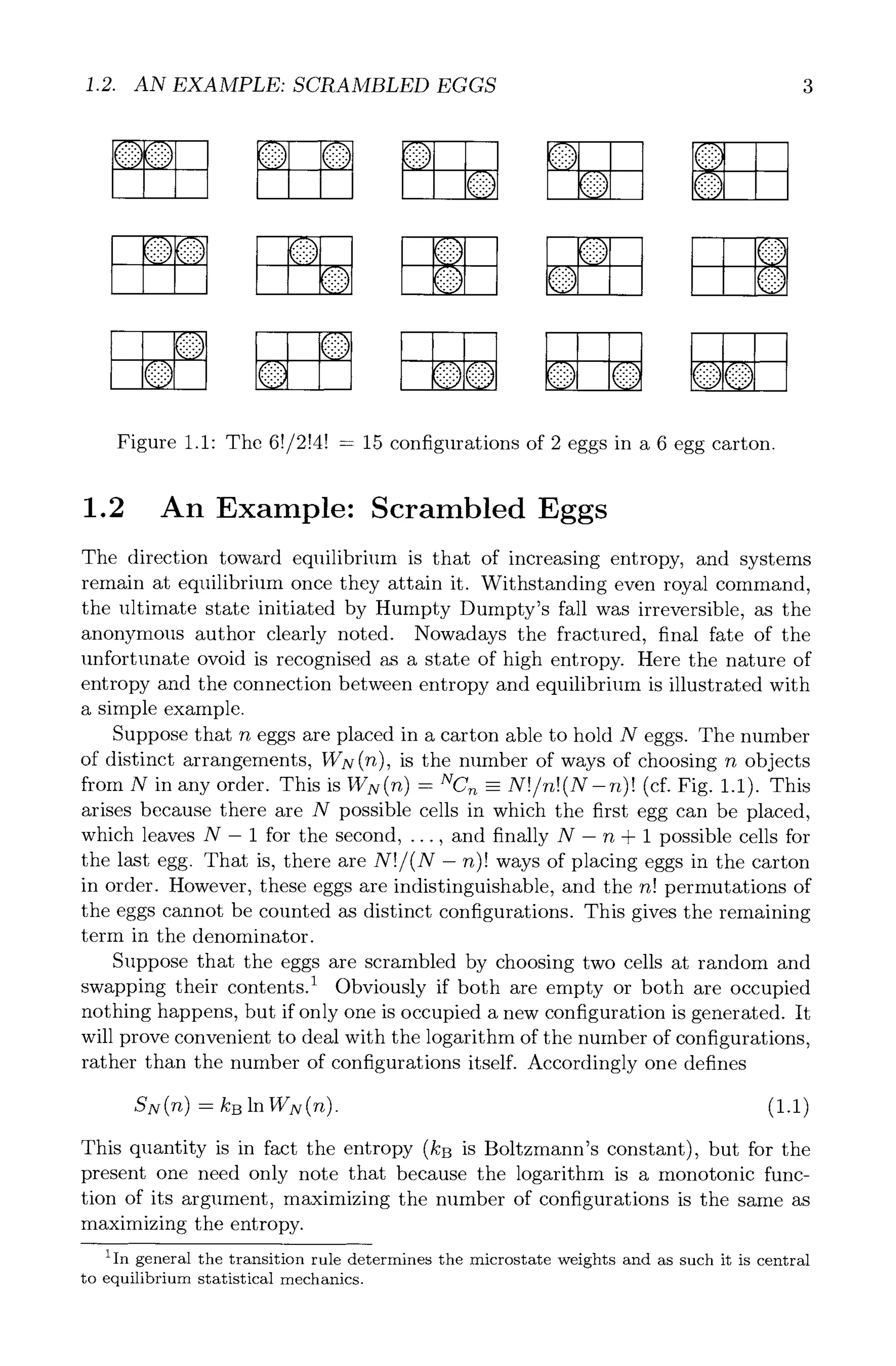
[(M- m)/M] = 2n(M- m)/(N + M) 2.
Conversely, the probability of an egg going from the second carton to the first is
2re(N-n)/(N + M) 2. For the equilibrium or steady state situation the net flux
must be 0, so these two must balance. The equilibrium number of eggs in each
carton is denoted by g and ~. Equating the fluxes, the equilibrium condition
is
m
Tt ?gt 7/, ?Tt
, or -- . (12)
N-~ M-m N M](https://image.slidesharecdn.com/2204562-250603055830-298e620c/75/Thermodynamics-And-Statistical-Mechanics-Phil-Attard-Auth-10-2048.jpg)
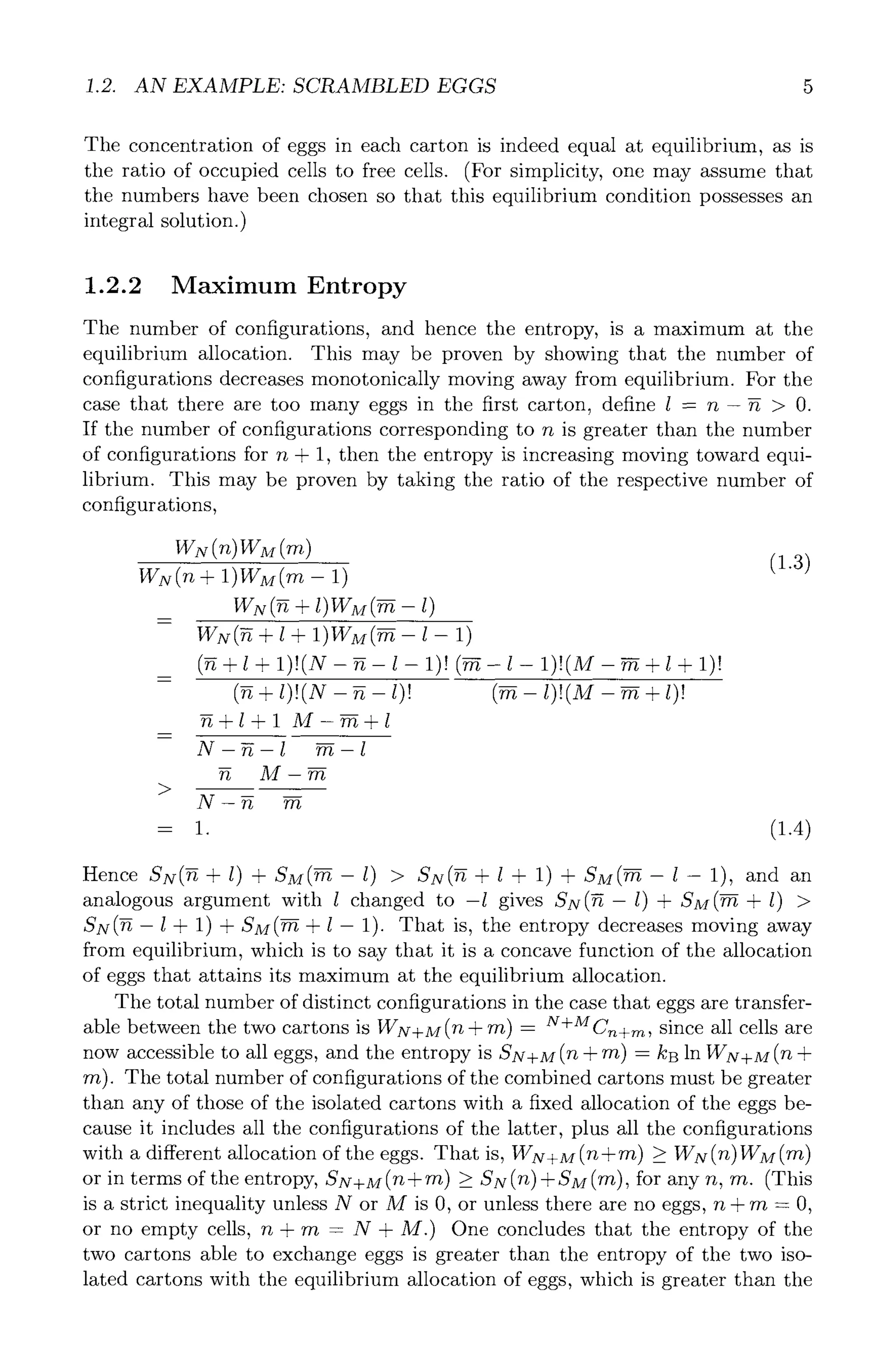
![6 CHAPTER 1. PROLOGUE
4.0E+08
3.5E+08 -
3.0E+08 -
2.5E+08-
2.0E+08-
1.5E+08-
1.0E+08 -
5.0E+07
0.0E+00
25
20-
15~
+ 10-
5-
0
9 9 0
AAAAA
I I I I
2 4 6 8 1012
A _~ t. t.
"F I I I I ~m
0 2 4 6 8 l0 12
Figure 1.2: The number of configurations as a function of the number of eggs in
the first carton, for a dozen eggs in total, n + m - 12, allocated to an ordinary
carton, N - 12, and a twin carton, M - 24. The inset shows the constrained to-
tal entropy, in units of kB, with the arrow indicating the equilibrium occupancy,
- 4, and the dotted line giving the unconstrained entropy, ln[36!/12! 24!] .
entropy of any other allocation of eggs to tile isolated cartons,
SN+M(n + m) 2 SN(g) + SM(57) 2 SN(n) + SM(m), (1.5)
where ~ + m - n + 'm, and ~/N - TFi/M. This behaviom" of tile constrained
entropy is shown in Fig. 1.2.
1.2.3 Direction of Motion
It has been shown that the equilibrium or steady state is tile one with the
maximum entropy, and now it is shown that the system out of equilibrium is
most likely to move in the direction of increasing entropy. The probability that
the N carton with n eggs will gain an egg, p(n + 1In ), is required. (Obviously
the other carton will simultaneously lose an egg, m + m- 1.) This was given
above in equating the fluxes to find the equilibrium state,
2m(X- n) (1.6)
p(n+lln )- (N+M) 2 "
Similarly,
p(n- lln ) --
(N + "
(1.7)](https://image.slidesharecdn.com/2204562-250603055830-298e620c/75/Thermodynamics-And-Statistical-Mechanics-Phil-Attard-Auth-12-2048.jpg)
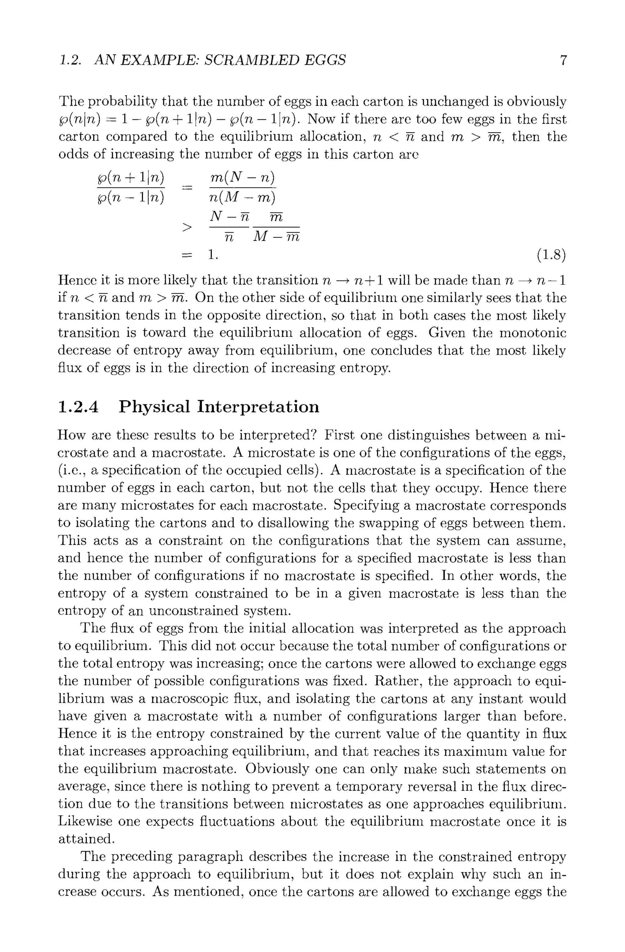

![1.3. BASIC NOTIONS 9
common, and distinct means that no two macrostates have the same value of
the observable. In addition to macrostates, there may exist states that are sets
of microstates but which are not disjoint or are not distinct.
The microstate that the system is in varies over time due to either determin-
istic or stochastic transitions. In consequence, transitions also occur between
the macrostates of the system. The set of all states that may be reached by a
finite sequence of transitions defines the possible states of the system. Hence
in time the system will follow a trajectory that eventually passes through all
the possible states of the system. A transition rule for the microstates may be
reversible (i.e., symmetric between the forward and the reverse transitions), but
will yield statistically irreversible behaviour in the macrostates over finite times.
1.3.2 Probability
A system may be considered in isolation from its surroundings. Its state is
specified by the values of certain fixed quantities such as size, composition,
energy, and momentum. Each of the microstates of a system has a nonncgative
weight that may depend upon the state of the system. It is conventional to take
the microstates of an isolated system to have equal weight, as in the ergodic
hypothesis or the hypothesis of equal a priori probability of classical statistical
mechanics, but it will be shown here that the formalism of statistical mechanics
holds even for nonuniformly weighted microstates. Ultimately the weight of the
microstates is determined by the transitions between them. It is the task of
statistical mechanics to identify explicitly the transition rule and to construct
the weights, whereas the formalism of statistical thermodynamics only requires
that the microstates and their weight exist.
The probability that the system is in a particular microstate is proportional
to its weight. That is, if the weight of the microstate labelled i is cvi, and the
total weight of the system is W = Y~i cvi, then the microstate probability is
0di
- _ .
W
Obviously the probability is normalised, Y~-iPi = 1. In the event that the mi-
crostates are equally weighted, then up to an immaterial scale factor one can
take the weight of the accessible microstates to be unity. (The inaccessible mi-
crostates may either be excluded from consideration, or else be given 0 weight.)
In this case W is just the total number of accessible microstates, and Pi = 1/W.
That is to say, uniform weight is the same as equal probability, and the proba-
bility of any one microstate is one over the total number of microstates. In the
general case, the microstate weights and the total weight are dependent on the
state of the system.
The theory of probability is ultimately founded upon set theory, which is
the reason that macrostates were introduced as sets of microstates. The weight
of a macrostate c~ is the sum of the weights of the corresponding microstates,
a~ = }-]ic~ czi-3 Consequently, its probability is the sum of the probabilities of
3Although mathematical symbolism provides a concise, precise way of communicating,](https://image.slidesharecdn.com/2204562-250603055830-298e620c/75/Thermodynamics-And-Statistical-Mechanics-Phil-Attard-Auth-15-2048.jpg)
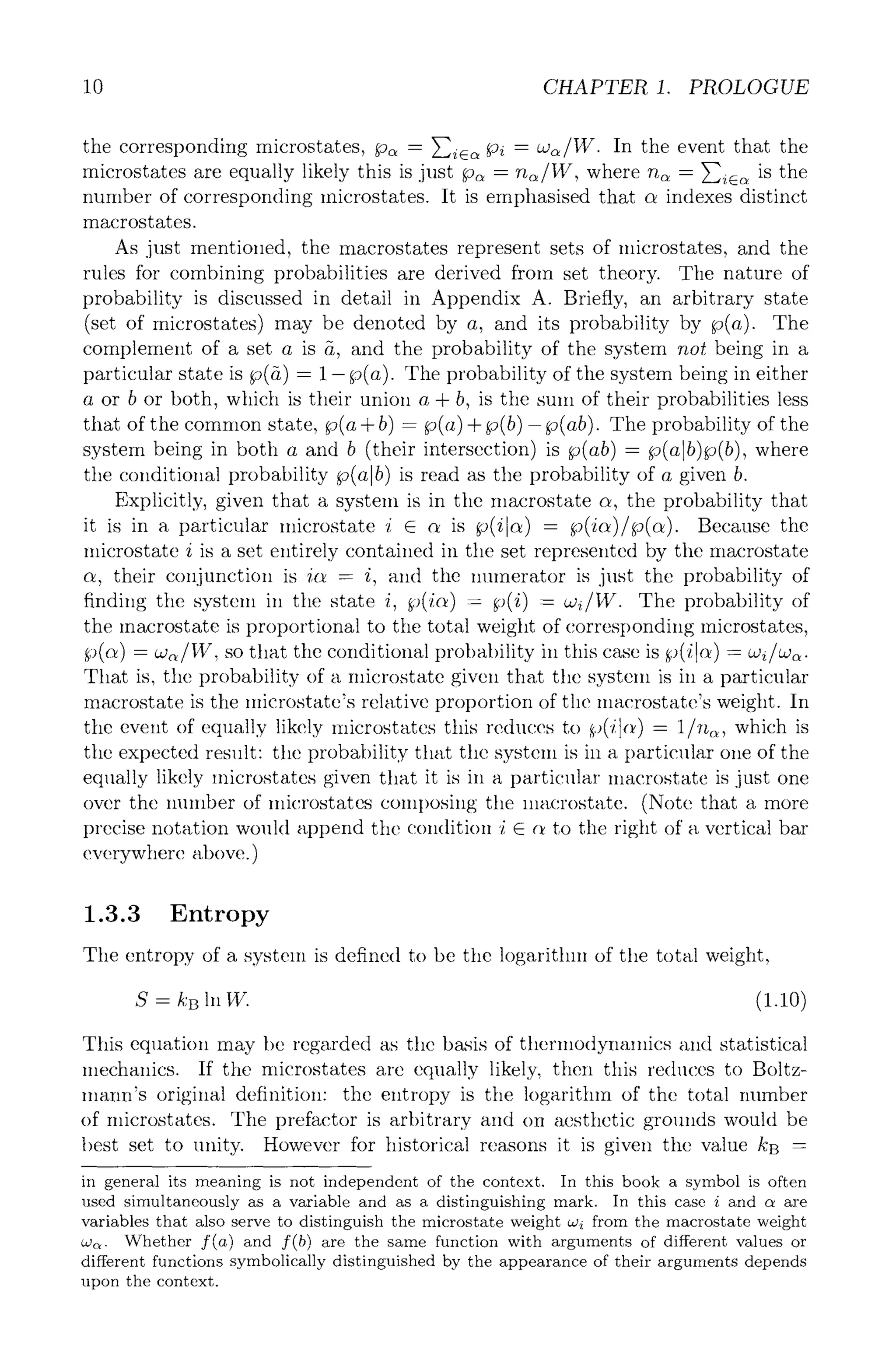
![1.3. BASIC NOTIONS 11
1.38 x 10.23 J K -1, and is called Boltzmann's constant. (It will be seen that
there is a close connection between entropy, energy, and temperature, which
accounts for the dimensions of entropy.)
By analogy, the entropy of a macrostate labelled c~ is defined as S~ =
kB lncJ~. Again for equally likely microstates this is just the logarithm of the
number of encapsulated microstates. One can also define the entropy of a mi-
crostate as Si = kB lnczi, which may be set to 0 if the microstates are equally
likely.
The important, indeed essential, thing is the weights; it was shown above
that these determine the probability of the microstates and macrostates. All of
thermodynamics and statistical mechanics could be derived without ever intro-
ducing entropy, since by the above formulae the two are equivalent. However
entropy is more convenient than the number of states because by definition it
is a linear additive property: the total weight of two independent subsystems
is Wtot~l = W1W2, whereas the total entropy is Stot~ = S1 + $2. Other linear
additive quantities include the energy, volume, and particle number. It will be
demonstrated in the following chapters that additivity is central to the formal
development of thermodynamics and statistical mechanics.
The relationship between entropy and disorder or unpredictability is revealed
by the interpretation of entropy as the number of equally likely microstates. If
the system is only ever found in a few states, then those states occur with high
probability: the system is said to be ordered or predictable, and it consequently
has low entropy. Conversely, if a system is equally likely found in any of a large
number of states, then it is quite disordered and unpredictable, and it has a
high entropy. The entropy of a system with only one state is defined to be 0,
and systems with more than one accessible state have an entropy that is strictly
positive.
The entropy of the system may be rewritten in terms of the probability
of the disjoint macrostates. (Note that the present treatment considers only
distinct macrostates, so that all the microstates corresponding to the value c~ of
the observable are collected together, which contrasts with many conventional
treatments in which different values of the index do not necessarily correspond to
different macrostates.) If macrostate c~ has weight ca~, probability p~ = a~/W,
and entropy S~ = kB ln w~, then the expression for the total entropy may be
rearranged as
S[p] = PBlnW
O..)c~
= kB E -~- in W
oz
= kBE~ lncz~+ln
oz
= E p~ [S~ - kB In Po~]. (1.11)
oz
This is the most general expression for the entropy of a system in terms of
the probabilities of disjoint macrostates. The first term in the brackets repre-](https://image.slidesharecdn.com/2204562-250603055830-298e620c/75/Thermodynamics-And-Statistical-Mechanics-Phil-Attard-Auth-17-2048.jpg)
![12 CHAPTER 1. PROLOGUE
sents the internal entropy of the macrostate, and the second term accounts for
the disorder due to the system having a number of macrostates available. The
internal entropy of the state c~ is S~ = kB In cz~, and it arises from the condi-
tional disorder or unpredictability associated with being in a macrostate, since
this is insufficient to delineate precisely the actual microstate of the system. If
the probability distribution is sharply peaked about one macrostate, then the
total entropy equals the internal entropy of this macrostate, since the second
term vanishes because in 1 = 0. One can replace the sum over macrostates
by a sum over microstates, S[p] = ~-~.iPi [Si - kB in Pi]. For equally likely mi-
crostates, Si = 0 and pi = l/W, it is clear that this immediately reduces to
Boltzmann's original result, S = kB in W. However, the derivation shows that
in all circumstances it reduces to Boltzmann's result anyway. This point must
be emphasised: in the general case of nonuniform microstates and macrostates,
the entropy is a physical property of the system (it is the logarithm of the
total weight) and its value is not changed by writing it as a functional of the
macrostate probability, or by how the microstates are grouped into macrostates.
In the literature one often sees the expression
Sos[p] - --kB E p~ In p~. (1.12)
This equation was originally given by Gibbs, who called it the average of the
index of probability. 4 It was also derived by Shannon in his mathematical the-
ory of communication, in which context it is called the information entropy. 5
Comparison with Eq. (1.11) shows that the internal entropy of the macrostate
is missing from this formula. Hence the Gibbs-Shannon entropy must be re-
garded as the 'external' part of the total entropy. It should be used with caution,
and depending upon the context, one may need to explicitly add the internal
contribution to obtain the full entropy of the system.
In the present approach to thermodynamics and statistical mechanics, the
only expressions for the entropy of the system that will be used are Eq. (1.10)
and Eq. (1.11). The Gibbs-Shannon expression, Eq. (1.12), is often invoked in
the principle of maximum entropy, 6 where it is used to obtain the macrostate
probability (by maximisation of the entropy functional). In the present for-
mulation, the macrostate probability may be trivially expressed in terms of
the macrostate entropy, namely it is proportional to the exponential of the
macrostate entropy,
_- (1.13)
P~= W Z '
4j. W. Gibbs, Elementary Principles in Statistical Mechanics Developed with Special Ref-
erence to the Rational Foundation of Thermodynamics, Yale Univ. Press, New Haven, CT,
1902; Dover, New York, 1960.
5C. E. Shannon and W. Weaver, The Mathematical Theory of Communication, Univ. of
Illinois Press, Urbana, 1949.
6E. T. Jaynes, Information theory and statistical mechanics, Phys. Rev. 106 (1957), 620;
108 (1957), 171. R. D. Rosenkrantz (Ed.), E. T. Jaynes: Papers on Probability, Statistics,
and Statistical Physics, D. Reidel, Dordrecht, 1983.](https://image.slidesharecdn.com/2204562-250603055830-298e620c/75/Thermodynamics-And-Statistical-Mechanics-Phil-Attard-Auth-18-2048.jpg)
![1.3. BASIC NOTIONS 13
where the normalising factor is
Z- ~ es~/kB = ~ ca~ - W. (1.14)
oe oL
This expression for the macrostate probability will be used throughout, although
it ought be clear that it is entirely equivalent to the original definition that
the probability is proportional to the number or weight of corresponding mi-
crostates.
The Continuum
It is often the case that the states are relatively close together so that it is
desirable to transform from the discrete to the continuum, as is necessary in
the case of classical statistical mechanics. It is only meaningful to perform such
a transformation when the state functions vary slowly between nearby states.
One could simply take the continuum limit of the discrete formulae given above,
transforming sums to integrals in the usual fashion, or one can derive the results
for the continuum directly, as is done here.
Represent the state of the system by x, a point in a multidimensional space,
and let ca(x) be the nonnegative weight density measured with respect to the
volume element dx. The total weight of the system is
W -- / dxca(x), (1.15)
and the total entropy is S = kB in W, as usual. The probability density is
ca(x) (1.16)
w'
with the interpretation that p(x)dx is the probability of the system being within
dx of x. Accordingly the average of a function of the state of the system is
(f} = f dxca(x)f(x).
One can define the entropy of the state of the system as
S(x) = kB in [w(x)A(x)], (1.17)
in terms of which the probability density is
eS(x)/kB
p(x)- LX
(x)-----W" (1.18)
Here A(x) is an arbitrary volume element introduced solely for convenience. (It
makes the argument of the logarithm dimensionless and gives the probability
density the correct dimensions.) Obviously the probability density is indepen-
dent of the choice of A(x), since the one that appears explicitly cancels with the
one implicit in the definition of the state entropy. The volume element has no
physical consequences and is generally taken to be a constant; equally, it could
be ignored altogether.](https://image.slidesharecdn.com/2204562-250603055830-298e620c/75/Thermodynamics-And-Statistical-Mechanics-Phil-Attard-Auth-19-2048.jpg)
![14 CHAPTER 1. PROLOGUE
The system entropy may be written as an average of the state entropy,
S = kB in W
-- /dxp(x)kB lnW
-- dx p(x)S(x) - kB In W
= ./dx p(x)IS(x) - kB in {p(x)A(x)}]. (1.19)
This is the continuum analogue of Eq. (1.11). Although the arbitrary volume
element appears explicitly here, it cancels with the corresponding term in S(x),
and the total entropy is independent of the choice of A(x).
The macrostates in the case of the continuum are generally represented by
hypersurfaces of the space. On the hypersurfaces particular observables that
depend upon the state of the system have constant values. Although concep-
tually similar to the discrete case, the treatment of continuum macrostates can
be more complicated in detail (see Ch. 5).
The formulae given above for entropy and probability are surprisingly pow-
erful, despite their evident simplicity and that of their derivation. All of thermo-
dynamics and statistical mechanics is based upon these results and the notions
that underlie them.
1.4 Reservoirs
1.4.1 An Example: Egg Distribution
The example explored above, which may seem paltry, is in fact quite rich, and
here it is used to introduce the reservoir formalism invoked throughout this
book. In the example, the microstates, which are the distinct arrangements
of eggs in the carton cells, are all equally likely, and the macrostates, which
are the number of eggs in each carton, have a probability in proportion to the
corresponding number of microstates. Hence the probability of there being n
eggs in the N carton, given that the other carton can hold M eggs and that
there is a total of n + rn eggs, is
- ~ NCn MC,,~. (1.20)
p(nlN, M, n + m) NCn MC'~/ ~:0
It was shown that the equilibrium allocation, g = N(n + rn)/(N + M), max-
imises the number of configurations, and this gives the peak of the distribution.
Taking the logarithm of the above probability distribution, and making Stir-
ling's approximation for the factorials, an expansion to second order about
gives a quadratic form that when reexponentiated approximates the distribution
by a Gaussian,
-N(M + N)(n- ~)2 (1.21)
p( lx, M, + Z -1 2 (N -](https://image.slidesharecdn.com/2204562-250603055830-298e620c/75/Thermodynamics-And-Statistical-Mechanics-Phil-Attard-Auth-20-2048.jpg)
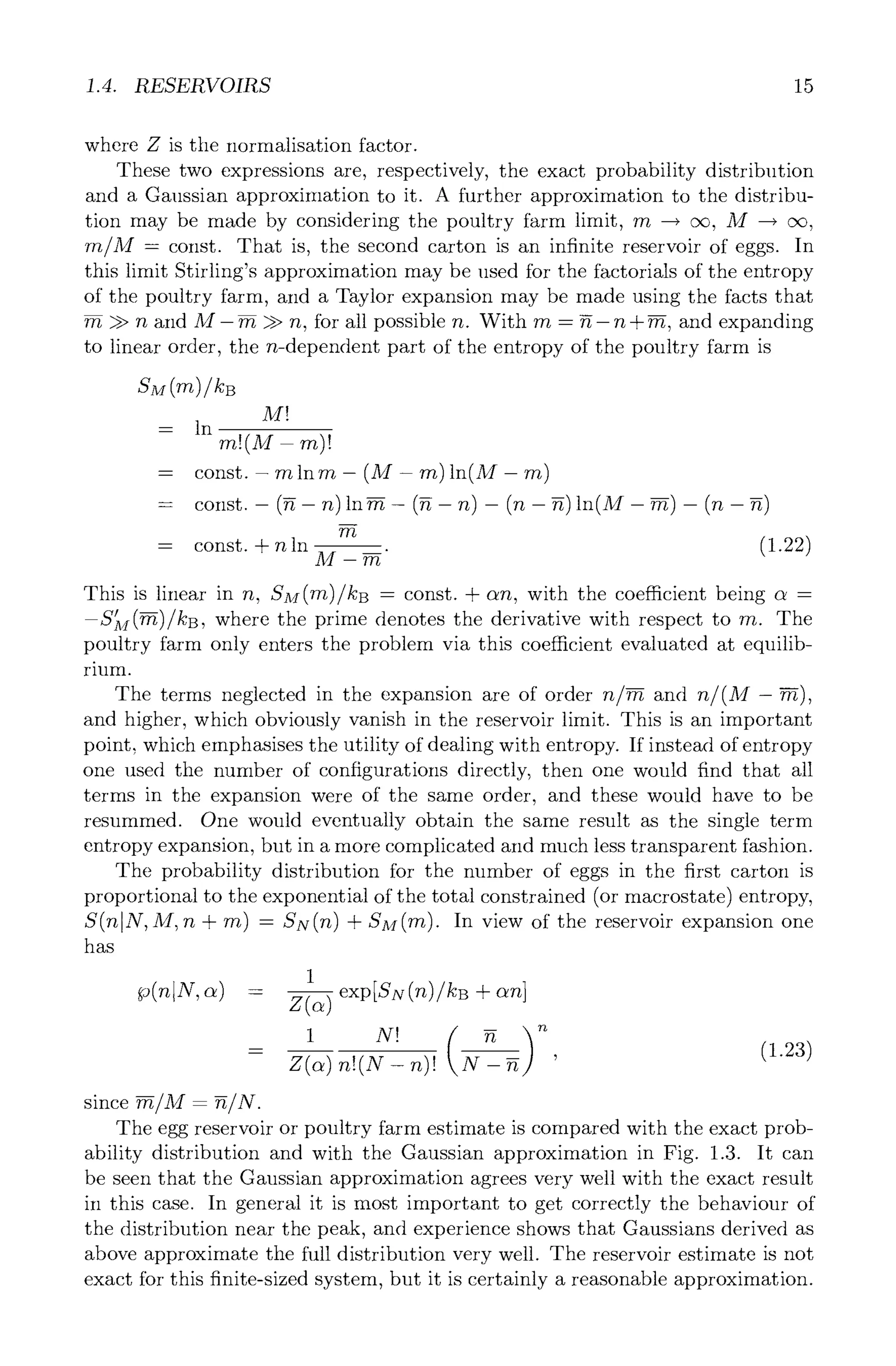
![16 CHAPTER 1. PROLOGUE
0.3
0.25 -
0.2 -
0.15
0,1 -
0.05
f-
0 2 4 6 8 10 12
Figure 1.3: The occupancy probability, p(nlN , M, n + m), of an ordinary carton
for a dozen eggs allocated between it and a twin carton, N = 12, M = 24
and n + m = 12. The symbols are the exact enumeration, the solid line is the
Gaussian approximation with ~7 = 4, and the dotted line results if the exchange
occurs with a poultry farm with c~ = ln[8/(24- 8)].
When one considers that one had no information about the size of the second
carton (or equivalently about the total mnnber of eggs), it is quite a revelation
to see how well it performs. The reservoir estimate must allow for all possible
M and m + n, which is why it is broader than the exact result for this particular
case (M = 24, m + n = 12). As the size of the second carton is increased (at
constant -~/M = g/N), the exact probability distribution becomes broader and
approaches the reservoir estimate.
1.4.2 The Reservoir Formalism
An overview of the reservoir approach in thermodynamics and statistical me-
chanics may be summarised as follows. The more detailed analysis will be
given in later chapters. Consider two systems in contact and able to exchange
an extensive quantity (such as energy or particles) that is in total conserved,
X l -t-X2 -- Xtotal. The probability distribution of the parameter for the first
system is proportional to the total weight of corresponding microstates (total
number if these are equally likely). Equivalently, it is proportional to the expo-
nential of the constrained total entropy,
1
gO(XllXtot~l) - ~y exp[S(xl)/kB + S(x2)/kB]. (1.24)](https://image.slidesharecdn.com/2204562-250603055830-298e620c/75/Thermodynamics-And-Statistical-Mechanics-Phil-Attard-Auth-22-2048.jpg)
![1.4. RESERVOIRS 17
This expression is true even when the systems are of finite size. It does however
assume that the interactions between the systems are negligible to the extent
that the total entropy is the sum of their individual entropies, Stotal = S(Xl) +
S(x2). The denominator Z ~ is just the normalising factor, which at this stage
is the unconstrained total entropy.
In the event that the second system is a reservoir, which means that Xl ~ 2;2,
a Taylor expansion of its entropy may be made about Xtotal and truncated at
linear order,
S(X2) -- S(Xtotal) -- Xl
0~(Xtotal)
(~Xtotal
The second term is of order Xl whereas the first neglected term goes like _2e,
, ~ID2 ~-~
O(x~/x2) (in general the entropy is extensive $2/x2 ~" O(1)). This is negligible
in the reservoir limit x l/x2 ~ O. The remaining neglected terms are analogously
of higher order.
The constant term, S(Xtotal), which is independent of the subsystem 1, may
be neglected (or, more precisely, cancelled with the identical factor in the de-
nominator). One may define field variables, like temperature and pressure, as
the derivatives of the entropy, A -- kBlOS(Xtotal)/(:C)Xtotal . The subscripts may
now be dropped, because the reservoir only enters via A, which has the physical
interpretation as the rate of change of its entropy with x. Hence the probability
distribution for the subsystem is now
1
- - (].26)
The equilibrium value of the exchangeable parameter, ~, is, by definition,
the most likely macrostate, and this is given by the peak of the probability
distribution. One has the implicit equation
Ox m
x--x
- a, (-,.27)
or in view of the definition of the field variable as the derivative of the entropy,
A(~) = A. On the left-hand side is the field variable of the subsystem, and
on the right-hand side is the field variable of the reservoir, and this says that
equilibrium corresponds to equality of the two.
The normalisation factor for the probability distribution is called the parti-
tion function, and it is of course
Z(A) - E eS(x)/kBe-Xx" (1.28)
x
The exponent is that part of the constrained total entropy that depends upon
the subsystem, Stotal(XlA) - S(x)/kB- Ax. The unconstrained, subsystem-
dependent, total entropy is
Stotal (/~) - Z ,(x ,X)[Sto a (Xl ) -- k.
x
= kB ]n Z(~), (1.29)](https://image.slidesharecdn.com/2204562-250603055830-298e620c/75/Thermodynamics-And-Statistical-Mechanics-Phil-Attard-Auth-23-2048.jpg)
![18 CHAPTER 1. PROLOGUE
and the average value of the exchangeable quantity is given by
(x} -- ~ p(xlA)x - - 0A " (1.30)
X
One should note that in the reservoir formalism three distinct entropies
appear: S(x) is the entropy of the isolated subsystem in the macrostate x,
Stot~l(xlA ) is the total entropy of the subsystem and reservoir when the subsys-
tem is constrained to be in the macrostate x, and Stot~(A) is the unconstrained
total entropy of the subsystem and reservoir. The latter two entropies do not
include the constant contribution to the reservoir entropy that is independent
of the presence of the subsystem.
One can of course generalise the formalism to include multiple extensive
parameters, some exchangeable and some fixed. One can extend it to finite-sized
reservoirs, where one must expand beyond linear order, and to systems in which
the region of interaction is comparable to the size of the subsystem, in which
case boundary terms enter. A linear additive conservative quantity is common,
but one can generalise the formalism, at least in principle, to the case that it is
not x itself that is conserved but some function of x, f(xl)dXl + f(x2)dx2 = 0.
In this case the reservoir field variable that enters the probability distribution
becomes A = []CB/(X)]-e0S(x)//Oqx.
Summary
Thermodynamics deals empirically with the macroscopic behaviour of bulk
matter, whereas statistical mechanics seeks to predict quantitatively that
behaviour from the interactions of atoms.
9 The equilibrium macrostate is that with the most microstates, and this
is the state of greatest entropy. A macroscopic flux is most likely in the
direction of increasing entropy.
All systems have a set of fundamental weighted microstates. Statistical
thermodynamics merely assumes the existence of the microstates and their
weights, whereas statistical mechanics constructs them from the transition
probabilities.
The entropy of a state is the logarithm of the total weight of correspond-
ing microstates. It may be expressed as a functional of the macrostate
probabilities.
The probability distribution of a parameter able to be exchanged with
a second system is proportional to the exponential of the total entropy
constrained by the value of the parameter. For a reservoir the constrained
total entropy equals the subsystem entropy minus the parameter times
the derivative of the reservoir entropy.](https://image.slidesharecdn.com/2204562-250603055830-298e620c/75/Thermodynamics-And-Statistical-Mechanics-Phil-Attard-Auth-24-2048.jpg)


![24 CHAPTER 2. ISOLATED SYSTEMS AND THERMAL EQUILIBRIUM
behaviour of a subsystem that is out of equilibrium. 2 The relationship with the
equilibrium thermodynamic potential or free energy is discussed below.
In general the constrained thermodynamic potential is defined as the neg-
ative of the reservoir temperature times the constrained total entropy. In the
present case the constrained thermodynamic potential for a subsystem of energy
E in contact with a heat reservoir of temperature T is
F(E N, V, T) = -TStotal (E]N, V, T)
= E - TS(E, N, V). (2.9)
By definition this is a minimum at equilibrium, and the energy flux of the sub-
system is down its gradient. By virtue of its close relationship to the constrained
total entropy, the constrained thermodynamic potential inherits many features
of the latter, such as the appropriate concavity and bijectivity. In particular,
the constrained thermodynamic potential is a convex function of energy, (and
also of number and volume), which follows from the concavity of the entropy
(F" - -TS" > 0). It is once more emphasised that the four arguments of the
constrained thermodynamic potential are independent.
The equilibrium thermodynamic potential or equilibrium free energy is defined
as the minimum value of the constrained thermodynamic potential, which in this
case obviously occurs at E- E(N, V, T),
F(N, V, T) - F(EtN , V, T) - E - TS(E, N, V). (2.10)
For the present case of constant temperature, this is called the Helmholtz free
energy, sometimes denoted by A(N, V, T). In this equation E is a dependent
variable, E(N, V, T), and consequently the Helmholtz free energy is a function
of jllst three independent variables. The entropy that appears on the right of
tile definition of the Helmholtz free energy is that of the isolated subsystem with
the equilibrium energy E. The overline on tile Hehnholtz free energy emphasises
that it is an equilibrium property.
The constrained thermodynamic potential clearly contains more informa-
tion than the equilibrium thermodynamic potential, since it is a function of
four independent variables, whereas tile equilibrium thermodynamic potential
is only a function of three. The constrained thermodynamic potenti~fl describes
the approach to energy equilibrium and energy fluctuations about the equilib-
rium state, whereas the equilibriuin thermodynamic potential only describes the
equilibrium state. The distinction made here between the two quantities is not
widespread in thermodynamics, and the present nomenclature is not necessarily
conventional. In most texts, the words 'thermodynamic potential' or 'free en-
ergy' in practice refer to equilibrium quantities. In the present work the strictly
~The properties of the constrained thermodynamic potential introduced here derive from
its intimate connection with the constrained total entropy. The basis of other nonequilibrium
potentials, such as the rather similar generalised Mathieu function and the Landau potential
used in expansions that describe criticality and phase transitions, is less clear. For an account
of these other potentials see H. B. Callan, Thermodynamics, Wiley, New York, 1960; L. D.
Landau and E. M. Lifshitz, Statistical Physics, 3rd ed., Pergammon Press, London, 1980; and
C. Kittel and H. Kroemer, Thermal Physics, 2nd ed., W. H. Freeman, New York, 1980.](https://image.slidesharecdn.com/2204562-250603055830-298e620c/75/Thermodynamics-And-Statistical-Mechanics-Phil-Attard-Auth-30-2048.jpg)

![26 CHAPTER 2. ISOLATED SYSTEMS AND THERMAL EQUILIBRIUM
temperature derivative of the Helmholtz free energy is
OF(N,V,T)
OT
OT N,V
OF(EIN, V,T)
OT E=-~
OF(EIN, V, T)
OT z=-E
= -S(E,N,V).
OF(EIN, V,T)
+
OE E=E
OE(N,V,T)
OT
(2.11)
The important point of this derivation is the passage from the second to the
third equality, where the final term vanishes, OF(E]N, V, T)/OE]E=-E -O, be-
cause of the optimal nature of the constrained thermodynamic potential at the
equilibrium state. This is a general feature that may be widely exploited. The
entropy in the final equality is that of the isolated subsystem with the equilib-
rium energy; it may be written S(N, V, T).
One sees that because the constrained thermodynamic potential is optimised
at equilibrium, differentiating the Hehnholtz free energy is tile same as differen-
tiating the constrained thermodynamic potential holding E fixed. It is for this
reason that one often sees the expression F - E- TS, and OF/OT - -S, it
being implicit that although the energy that appears here is really E(N, If, T),
it may be held fixed during any differentiations. The entropy may similarly
be held fixed as far as temperature differentiations goes because it is really
S(N, V, T) - S(E(N, V, T), N, V), and E may be held fixed.
The other derivatives of tile Helmholtz free energy follow directly from the
corresponding derivatives of the entropy for an isolated systeln, holding E fixed.
They give the pressure
(olN
OV T,N
oF(z x, v,T))
OV -E,T,N
= _T(OS(E'N'V))
OV f ,N
- - - - --p~ (2.12)
and the chemical potential
OF(N,V,T))
ON T,V
= (OF(EIN'V'T))
ON --E,T,V
= _T(OS(E'N'V))
ON -~,v
(2.13)](https://image.slidesharecdn.com/2204562-250603055830-298e620c/75/Thermodynamics-And-Statistical-Mechanics-Phil-Attard-Auth-32-2048.jpg)
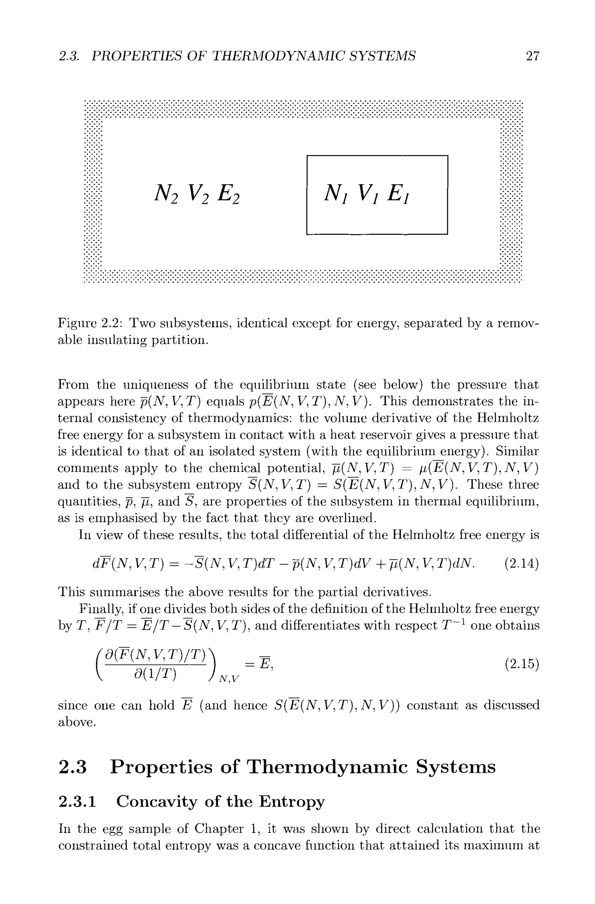
![28 CHAPTER 2. ISOLATED SYSTEMS AND THERMAL EQUILIBRIUM
the equilibrium macrostate. Using the notions of the extensivity of the entropy
and its maximisation at equilibrium, it is now demonstrated in general that the
entropy is a concave function of its arguments.
Consider two systems, identical except for energy, isolated from each other
by an insulating partition (Fig. 2.2). They have volume VI - 1/2 - V, number
of particles N1 - N2 - N, and energies E1 and E2. Their entropies are $1 =
S(E1, V, N) and $2 - S(E2,V,N), and the total entropy with the partition in
place is Stotal -- S1 -t- $2. This follows because the systems are isolated from
each other, and in such cases the entropy is a linear additive quantity. If the
insulating partition is removed, energy irreversibly flows from the more to the
less energetic system. The total entropy at the end of this process must be
greater than at the beginning,
StotM(J~l -+-Z2, 2V, 2N) ~ S(J~I, V, N) -+-S(J~2, V, X). (2.16)
This is simply a statement of the second law of thermodynamics, namely that
energy flows in the direction of entropy increase. The microscopic interpretation
is of course that relaxing the constraint imposed by the partition increases the
number of microstates available to the system. From symmetry equality is
expected if, and only if, E1 - E2. After equilibration the insulating partition
can be reinserted, and tile energy of each subsystem is (El + E2)/2, fluctuations
about this value being relatively negligible. This equilibrium division of the
energy between the two systems corresponds to the maximum entropy. Since
there is no further energy flow, the removal and insertion of the partition is now
a reversible process, and one must have
St~ El+E2 )
,V,N . (2.17)
Combining these two equations one obtains
( ) 1
S E1 -~-E2 V, N > [S(E 1 V, N) -+-S(E 2 V, N)] (2 18)
- - - 5 - - - ' ' ' " 9
The case E1 - E2 is here excluded, so that tile left side is strictly greater
than the right. This says that any chord to the entropy curve lies below the
curve, which defines a concave flmction. By performing a Taylor expansion as
E1 --+ E2, it may be seen that this is equivalent to
(09S(E, V,N)) <0. (2.19)
OE2 V,N
The above explicitly shows that the entropy of a system is a strictly concave
function of energy. It is clear that analogous steps can be carried out individually
for volume and for particle number, so that in general the entropy is a concave
function of its arguments.
Simultaneous variations are hardly more complicated. Suppose that two
isolated systems are identical apart from their energies and volumes. Allowing
simultaneous exchange of both as above, one concludes that
( ) 1
Stotal E1 -~-E2 Vl -~-V2 N > [S(E 1 V1 N) -~-S(E 2 V2 N)] (2."20)
2 ' 2 ' 2 ' ' ' ' "](https://image.slidesharecdn.com/2204562-250603055830-298e620c/75/Thermodynamics-And-Statistical-Mechanics-Phil-Attard-Auth-34-2048.jpg)


![3.2. CONSTANT CHEMICAL POTENTIAL 37
••••.•••.•.•.•.•••••.•••••••••••.•.•.•.•.•.•.•••.•.•••••.•.•.•.•.•.•.•.•.•.•.•.•••.•.•••••.•.•••••.•.•.•.•.•.•.•.•.•.•.•••.•••••.•.•.•.•.•.•.•.•.•.•.•.•.•.•.•.•.•.••:::::::::::::::::::::::
"o~ ",',-o'o'.'o" ~176176176" "o~176 ",'o~176 ~ ~176 ".'o~176176176 ~176176176176176176176176176
"o'o'o" " ~176176
" "o~ ~176176 " ".'.~176 ~176176176176176
iiii!
!! i
:::::::: r ::::::::::
. . . . . . . . .
. . . . . . . . .
. . . . . . . . .
. . . . . . . . .
. . . . . . . . .
. . . . . . . . .
. . . . . . . . .
. . . . . . . . .
. . . . . . . . .
. . . . . . . . .
iii::::iii N2 V2 E2 V1 Ez i::iiiii::!!
9oO...oo .....
9 .,~ .o.....oO.
9~176176 -~176176176
~176176176176 %~176176176176176176176
~176176176 ~176176176176176
%%~176 -.-.-.%%
%... %.....~176176
9 ..% %.~176176176176176
~176176 %~176176176176
~176176176176 ~176176176176176176
%~176176176176176 .....
~176176176176176 ~176176176
~176176176176176
. . . . . . . . . . . . . . . . . . . . . . . . . . . . . . . . . . . . . . . . . . . . . . . . . . . . . . . . . . . . . . . . . . . . . . . . . . . . . . . . . . . . . ~176176176176176
9o. 9 oo.o.......oo.o.......o..O.Oo.o. 9 ooo 9 9 ~176176176176176176176176176176176176176176176176176176176176176176176176176176176176176176176176176176176176
Figure 3.1: A subsystem 1 able to exchange energy and particles with a reservoir
2.
Stotal -- $1 -Jr-$2. The equilibrium energy and particle number partitioned
between the two systems are determined by the temperature and chemical po-
tential, as will now be shown. Because the reservoir is so large, the Taylor
expansion of its entropy may be truncated at the linear order,
$2(E2 V2 N2)- S2(Etota] 172 N)_-:-:-E~ #2 (3.3)
, , , , ,/ +,/ N1.
Neglecting the part independent of subsystem 1, and dropping the subscripts,
the constrained total entropy is
E #
Stot~l(N, El# , V, T) -- S(E, If, N)- -~ + -~N. (3.4)
This gives the total entropy for a subsystem in a nonequilibrium state of energy
E and particle number N, when in contact with a reservoir of temperature T
and chemical potential #.
The derivatives of the constrained total entropy are
OSota(N, E v,T) v, N)
= § (3.5)
ON T(E,V,N) T'
and
OStotal(N, El#, If, T) 1 1
= (3.6)
OE T(E,V,N) T"
The first term on the right-hand side is the derivative of the subsystem entropy,
which is the subsystem chemical potential and temperature, respectively. The
constrained total entropy is of course a maximum at equilibrium, which cor-
responds to the vanishing of these derivatives. This condition gives implicit
equations for the equilibrium energy E(#, V,T) and the equilibrium particle
number N(#, If, T), namely T(E, If, N) -- T and #(E, V, N) -- #. That is, at
equilibrium a subsystem that can exchange energy and particles with a reservoir
has the same temperature and chemical potential as the reservoir.](https://image.slidesharecdn.com/2204562-250603055830-298e620c/75/Thermodynamics-And-Statistical-Mechanics-Phil-Attard-Auth-42-2048.jpg)
![38 CHAPTER 3. VARIOUS RESERVOIRS
The direction of particle flow in the nonequilibrium case depends upon the
change in constrained total entropy with particle number, dStotal - [-#(E, V, N)
/T(E, V, N)+ #/T]dN (at constant volume and energy). Since the total entropy
must increase, dStot~l > 0, particles flow to the region of lower chemical poten-
tial (for a system at the same temperature as the reservoir). In other words, an
increase in the chemical potential of the reservoir will force more particles into
the system.
As for the isothermal system, one defines a constrained thermodynamic po-
tential that is the negative of the total entropy times the temperature,
~(Z, Nip , V,T) = -TStot~(E, NIp, V,T)
= z - TS(Z, V, N) - ~X
= F(E N, V, T) - ~N. (3.7)
From the concavity of tile subsystem entropy, tile constrained thermodynamic
potential is obviously a convex function of N and of E, and it is minimised by
their equilibrium values. Thus it represents the appropriate variational prin-
ciple for a nonequilibrium system able to exchange energy and particles with
a reservoir characterised by chemical potential # and temperature T. As fore-
shadowed above, it has the appearance of a Legendre transform with respect to
N of the constrained thermodynamic potential of a closed system in thermal
contact with a reservoir.
In the case of rapid thermal equilibration, one could take a:(N #, V, T) -
f~(E(N, V, T), Nlp, V, T) - F(N, V, T)- #N. This has the appearance of a
Legendre transform of the equilibrium free energy of a constant temperature
closed system (the Hehnholtz free energy), and represents a variational principle
for a system at the same temperatlu'e as the reservoir, but not in diffusive
equilibrium with it.
The constrained thermodynamic potential is minimised by the equilibrium
values of the energy E(#, V,T) ~tnd the number N(#, If, T). In the first place
O~(E, NIp , V, T) /OE - 1 - TOS(E, N, V)/OE - 0 when T(E, If, N) - T or at
the energy given by E - E(N, V, T), as found previously. Further,
O~(E, N p, V, T) : -T OS(E, N, V) _ #, (3 8)
ON ON
which vanishes at #(E, V,N) - p, which again is an implicit equation for
N - N(E, V, #). These are the two equations that determine the equilibrium
quantities E(#, V, T) and N(#, V, T).
From the concavity of the entropy it follows that the constraine(t thermody-
namic potential is a convex function of particle number, f~" - -TS" > 0. The
equilibrium thermodynamic potential or free energy of an open system, which
is called the grand potential, equals the minimum value of the constrained ther-
modynamic potential,
f~(#, V, T) - a(E, NI~,v, T)
= F(N, If, T) - #N. (3.9)](https://image.slidesharecdn.com/2204562-250603055830-298e620c/75/Thermodynamics-And-Statistical-Mechanics-Phil-Attard-Auth-43-2048.jpg)
![40 CHAPTER 3. VARIOUS RESERVOIRS
3.3 Constant Pressure
Now the effects of variable volume are analysed for a subsystem in contact
with a reservoir at constant pressure (an isobaric system). Consider an isolated
total system consisting of two isolated subsystems separated by a moveable,
diathermal partition (i.e., the partition is heat conducting). Thus the total
energy Etotal - E1 + E2 and volume Vtotal - V1 + 1/2 are fixed, but not their
partitioning between the two systems. The second system is an energy and
volume reservoir, and so a Taylor expansion is made for its entropy. This yields
for the subsystem-dependent part of the total entropy Stot~ - $1 + 8'2
E pV (3.17)
Stotal(E, VIN, p, T) - S(E, N, V) T T '
where p and T are the pressure and temperature of the reservoir. This is the
entropy of a subsystem out of equilibrium with respect to energy and volume.
Since the entropy must increase, the volume changes such that 0 < dStotal -
(p(E, V,N)/T(E, If, N)- p/T)dV. That is, if the system is in thermal but
not mechanical equilibrium, the volume of the system increases if its internal
pressure is larger than the external pressure of the reservoir.
The total entropy is maximised at equilibrium, which determines the energy
E(N, p, T) and the volume V(N, p, T) of the system. As previously one develops
a minimisation procedure for equilibrium by defining a constrained thermody-
namic potential that is the negative of the temperature times the total entropy,
G(E, V N,p,T) -- E - TS(E,N, V) + pV
= F(EIN, V,T)+pV. (3.18)
This is a convex function of the system volume and energy, and is tile appropriate
nonequilibrium potential for a system with moveable diatherlnal walls in contact
with a reservoir of fixed temperature and pressure. In the case of thermal equi-
librium having been established, one would take g(VIN ,p, T) - F(N, V, T)+pV
as the appropriate constrained thermodynamic potential that controls volume
equilibration.
Minimising G(E, VIN, p,T ) with respect to energy gives T(E, If, N) -- T,
which gives the equilibrium energy for a given volume, E(N, 17,T). Minimis-
ing with respect to vohune gives p(E, V, N)/T(E, V, N) - p/T, which gives the
volume for a given energy of the system and temperature and pressure of the
reservoir, V(EIN, p, T). Simultaneous solution of the two gives the full equi-
librium quantities, E(N,p,T) and V(N,p, T). The latter quantity also follows
directly from the minimisation of the thermally equilibrated constrained ther-
modynamic potential, Og(VIN, p, T)/OV- O, or
OF(N,V,T)
OV V=V
= -p (3.19)
In view of the convexity of G, the Gibbs free energy is defined as the minimum
value of the constrained thermodynamic potential,
G(N,p,T) - G(V,E]N,T,p)](https://image.slidesharecdn.com/2204562-250603055830-298e620c/75/Thermodynamics-And-Statistical-Mechanics-Phil-Attard-Auth-45-2048.jpg)
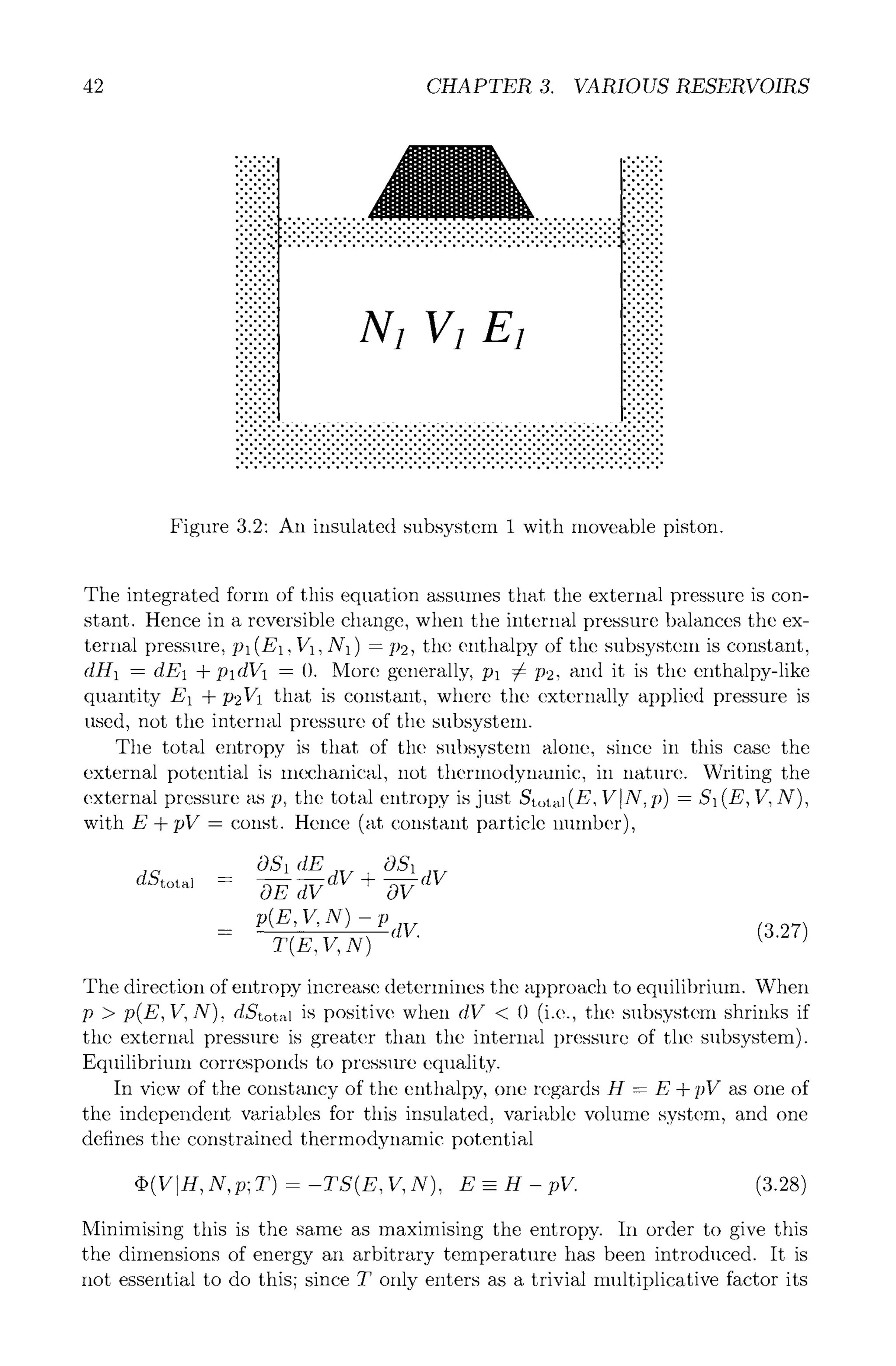


![3.6. THERMODYNAMIC SECOND DERIVATIVES 47
Here X could stand for E, N, or V, or it could be an additional parameter of
the system. The subsystem-dependent part of the total entropy of a subsystem
plus reservoir at x and T, for exchange of X, is
xX
Stotal(Xlx) - S(X) T (3.49)
As above, the total entropy is a concave function of the extensive variable,
< 0
OX2 x
The equilibrium value of X is X(x) (or more fully X(x, T)), and this gives the
maximum total entropy, Stotal(X) -- Stotal (X (x) Ix). It is now proven that this
latter quantity is a convex function of the reservoir field x/T.
One has
d2Stotal(X(x)]x) d aS(X) dX x dX 1
d(x/T) 2 = d(x/T) OX d(x/T) T d(x/T) - X(x) J
_
_ _ d X ( z ) , (3.51)
d(~/T)
where the cancellation occurs because x(--X(x)) - x and T(--X(x)) - T. (On the
left-hand side of each of these equations appears a property of the subsystem,
and the quantity on the right-hand side is a property of the reservoir.) Now
the equilibrium value is X, and if X t is any other value, then by definition
Stota 1(X t x) < Stotal (Nix), or
xX xX ~
< S(X)- S(X'). (3.52)
T T
An expansion to second order about X ~yields
so that
s(X) - s(x') + (x - x')s~(x') +
s(x') + (x - x')_-, +
T
(X-X') 2
2
(x-x') ~
Sxx(X')
Sxx(X'), (3.53)
~'] (x- x') ~
~-~-7 (X- X') < 2 Sxx(X'). (3.54)
Since the right-hand side is negative due to the concavity of the entropy, dividing
by (X - X~) 2 and taking the limit yields
a(~/T)
< 0, (3.55)
dX
or equivalently
dX
< 0. (3.56)
d(~/T)](https://image.slidesharecdn.com/2204562-250603055830-298e620c/75/Thermodynamics-And-Statistical-Mechanics-Phil-Attard-Auth-52-2048.jpg)