
Recommended
Recommended
More Related Content
Similar to The U.S. DeficitDebt Problem A Longer-Run PerspectiveD.docx
Similar to The U.S. DeficitDebt Problem A Longer-Run PerspectiveD.docx (16)
More from christalgrieg
More from christalgrieg (20)
Recently uploaded
Recently uploaded (20)
The U.S. DeficitDebt Problem A Longer-Run PerspectiveD.docx
- 1. The U.S. Deficit/Debt Problem: A Longer-Run Perspective Daniel L. Thornton The U.S. national debt now exceeds 100 percent of gross domestic product. Given that a significant amount of this debt is the result of governmental efforts to mitigate the effects of the financial crisis, the recession, and the anemic recovery, it is tempting to think that the debt problem is a recent phenomenon. This article shows that the United States was on a collision course with a major debt problem for nearly four decades before the financial crisis. In particular, the debt problem began around 1970 when the government decided to significantly increase spending without a corresponding increase in revenue. The analysis suggests that the debt problem cannot be permanently resolved without creating a mechanism to prevent the government from running persistent deficits in the future. (JEL E62, H62, H63) Federal Reserve Bank of St. Louis Review, November/December 2012, 94(6), pp. 441-55. T he U.S. debt has surpassed 100 percent of gross domestic product (GDP). This debt burden is due in part to the extremely large deficits incurred by attempts to mitigate the effects of the financial crisis, the relatively deep and prolonged recession, and the
- 2. anemic economic recovery. Given the emphasis on the financial crisis and its aftermath, it is important to realize the U.S. deficit/debt problem began over four decades ago. This longer- run perspective suggests that the recognition of the seriousness of the problem and the need for fundamental change eventually would have occurred. The recent financial crisis merely brought the U.S. deficit/debt problem to the public’s attention sooner rather than later. The analysis here shows that the U.S. deficit/debt problem began during the early 1970s when the government started to increase spending significantly without a corresponding increase in tax revenue. This article also analyzes various aspects of government revenues and expenditures to better understand the different elements of the debate on preventing the U.S. deficit/debt problem from becoming the U.S. deficit/debt crisis.1 Daniel L. Thornton is a vice president and economic adviser at the Federal Reserve Bank of St. Louis. The author thanks Clemens Kool for helpful comments. © 2012, The Federal Reserve Bank of St. Louis. The views expressed in this article are those of the author(s) and do not necessarily reflect the views of the Federal Reserve System, the Board of Governors, or the regional Federal Reserve Banks. Articles may be reprinted, reproduced, published, distributed, displayed, and transmitted in their entirety if copyright notice, author name(s), and full citation are included. Abstracts, synopses, and other derivative works may be made only with
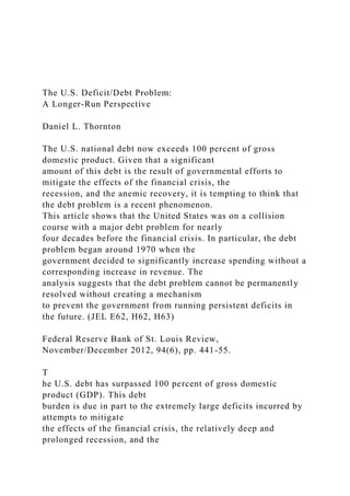
- 3. prior written permission of the Federal Reserve Bank of St. Louis. Federal Reserve Bank of St. Louis REVIEW November/December 2012 441 THE U.S. DEFICIT/DEBT PROBLEM: WHEN DID IT BEGIN? A long-run perspective on U.S. government deficits is helpful in understanding the current deficit/debt problem. Figure 1 shows the history of U.S. budget surpluses/deficits from 1800 through 2011 and Congressional Budget Office baseline budget projections up to 2020. Three aspects of this figure are noteworthy. First, until the recent financial crisis, large deficits have been associated with great wars—the War of 1812, the Civil War, and World Wars I and II. The only large peacetime deficit occurred in 1933 during the Great Depression, when the deficit hit a peak of 6.6 percent of GDP. In contrast, the deficits for 2009, 2010, and 2011 have all exceeded 8.7 percent. Second, each large deficit was followed by a period of budget surpluses or very small deficits. Indeed, with the exception of major wars and the Great Depression, the deficit relative to GDP averaged essentially zero. Third, a marked change in the behavior of the deficit occurred circa 1970. For the decade preceding 1970, the United States also had fairly persistent deficits, but they were relatively
- 4. small—on average, 0.8 percent of GDP. In contrast, the deficit averaged 2.1 percent for the 1970s, 3.9 percent for the 1980s, 2.2 percent for the 1990s, and 3.0 percent for the 2000s. Over the entire 1970-2010 period the deficit averaged 2.8 percent of GDP. The effects of the wartime deficits and peacetime surpluses are reflected in the size of the debt relative to GDP. Figure 2 shows the federal debt as a percent of GDP since 1840. The debt rose dramatically relative to GDP during the Civil War but declined more or less continuously Thornton 442 November/December 2012 Federal Reserve Bank of St. Louis REVIEW –30 –25 –20 –15 –10 –5 0 5 10
- 5. 1800 1820 1840 1860 1880 1900 1920 1940 1960 1980 2000 2020 Actual 2011 Projection 2000 Projection 1800 to 1990 = GNP 1991 to 2020 = GDP Percent War of 1812 Civil War WWI WWII Figure 1 The Federal Surplus/Deficit as a Percent of GNP/GDP NOTE: GNP, gross national product. SOURCE: The baseline budget projections to 2020 are from the Congressional Budget Office. until the United States entered WWI, when the percentage again peaked at the Civil War level. The percentage again declined until the Great Depression and WWII, when it rose dramatically
- 6. to a peak of 121 percent in 1946. After WWII the deficit as a percent of GDP declined nearly monotonically before leveling out around 1970. Because the deficit grew faster than GDP on average over the 1970-2007 period, the percent of GDP increased from 36 percent in 1970 to 64 percent in 2007, the highest peacetime level in U.S. history. Since 2007, the debt has increased to more than 100 percent of GDP. The large and persistent deficits over the 38 years preceding the financial crisis suggest that the United States would have had a serious deficit/debt problem without the financial crisis and recession. A back-of-the-envelope calculation suggests that had the United States continued on the path it was on, the country would have achieved a debt-to- GDP ratio of 100 percent around 2017. The recent events merely forced the recognition of the reality of the situation sooner rather than later. Indeed, several economists and market analysts issued warnings of an impending debt crisis (see Gokhale and Smetters, 2003; Kotlikoff and Burns, 2012; and references therein). The conclusion that the United States was on a collision course with a debt problem is sup- ported by a simple analysis of government revenues and expenditures as a percent of GDP.2 Figure 3 presents government spending and revenue as a percent of GDP from 1950 through 2010. The black and blue dashed lines denote the average federal government revenue and expenditures, respectively, as a percent of GDP from 1950 through 1969. The figure shows that after 1970 both revenues and expenditures increased on average
- 7. relative to the previous two decades; however, revenue increased marginally, while expenditures increased significantly. Revenue averaged 18.2 percent of GDP for the 1970-2007 period compared with 17.5 percent Thornton Federal Reserve Bank of St. Louis REVIEW November/December 2012 443 0 20 40 60 80 100 120 140 1840 1850 1860 1870 1880 1890 1900 1910 1920 1930 1940 1950 1960 1970 1980 1990 2000 2010 Percent Figure 2 Gross Government Debt as a Percent of GDP
- 8. SOURCE: Historical Statistics of the United States, Office of Management and Budget, and Haver Analytics. for the 1950-69 period, while expenditures averaged 20.6 percent and 18.1 percent, respectively, for the same two periods. On average, the government spent 2.4 percent of GDP more than it received in revenue during the 38-year period. Figure 3 shows, however, that tax revenue as a percent of GDP increased from 17.5 percent of GDP to 20.6 percent of GDP from 1993 to 2000. This increase is associated with the tax increases introduced in 1993. Revenue subsequently decreased following passage of the Economic Growth and Tax Relief Reconciliation Act of 2001 (EGTRRA; a.k.a. the George W. Bush tax cuts). The decline in tax revenue relative to GDP between 2000 and 2003 was likely due in part to the 2001 recession; 2007 tax revenue as a percent of GDP was at or above the 1950-69 average level during the 2006-08 period. The marked decline in revenue as a percent of GDP during the 2009-11 period is likely due to the financial crisis and the accompanying recession. Hence, while the Bush tax cuts may have been a contributing factor to the deficit after 2001, this analysis sug- gests that the average deficit from 1970 to 2007 was largely due to a marked increase in expendi- tures relative to GDP: The ratio of debt to GDP was 57 percent in 2000 and increased to only 64 percent by 2007. Hence, most of the increase in the debt over the entire 1970-2007 period occurred because the government spent much more than it
- 9. collected in taxes—about $6 trillion more. Sources of Government Spending What components of government spending account for the increase in spending during the 1970-2007 period? The answer to this question is shown in Figure 4, which shows federal spend- Thornton 444 November/December 2012 Federal Reserve Bank of St. Louis REVIEW 0 5 10 15 20 25 30 1950 1955 1960 1965 1970 1975 1980 1985 1990 1995 2000 2005 2010 Revenue/GDP Expenditures/GDP
- 10. Average Revenue (1950-69) Average Expenditures (1950-69) Percent Figure 3 Revenue and Expenditures as a Percent of GDP (1950-2010) Thornton ing as a percent of GDP by categories from 1950 through 2010. The categories are defense spend- ing (DS), interest paid on the public debt (IPD), Social Security and Medicare/Medicaid (SSM), other payments to individuals (OPI), and other federal expenditures (OFE). The figure shows that IPD and OFE have been relatively small and relatively constant over the period, with no discernible trend. Hence, the marked increase in spending cannot be due to IPD or OFE. It also appears that DS cannot account for the spending increase as it has generally trended down over the sample period ever since the late 1960s. The figure shows that SSM and OPI are the main spending drivers over the 1970-2007 period. These expenditures accounted for 5 percent of government spending as a percent of GDP in 1950 and had increased to only 6.1 percent of GDP by 1969. However, SSM and OPI spending as a percent of GDP doubled by 2007 to 12.1 percent of GDP. SSM and OPI spending increased
- 11. by another 3.6 percentage points of GDP by 2010 to 15.7 percent of GDP. The analysis above shows that OPI and SSM account for essentially all of the increase in government spending that has given rise to the deficit/debt problem. This section analyzes gov- ernment spending in more detail to better pin down the source of the spending. Figure 5 shows the percent of total federal spending annually from 1979 through 2011 by three categories: discretionary spending, mandatory spending, and interest payments on the national debt. Mandatory spending includes Social Security payments, Medicare, Medicaid, income security, other retirement and disability spending, and all other mandatory spending. Income security includes unemployment compensation, Supplemental Security Income, the refundable portion of the earned income and child tax credits, supplemental nutrition assistance, Federal Reserve Bank of St. Louis REVIEW November/December 2012 445 0 2 4 6 8
- 12. 10 12 14 16 1950 1955 1960 1965 1970 1975 1980 1985 1990 1995 2000 2005 2010 Defense IPD = Interest Paid on the Public Debt SSM = Social Security and Medicare/Medicaid OPI = Other Payments to Individuals OFE = Other Federal Expenditures Percent Figure 4 Federal Spending as a Percent of GDP by Categories (1950- 2010) family support, child nutrition, and foster care. The figure shows that the decline in discretionary spending as a percent of total government spending was essentially matched by an increase in mandatory spending. Discretionary spending decreased from 48 percent to 37 percent of total
- 13. government spending between 1979 and 2011, while mandatory spending increased from 44 percent to 56 percent of total spending. Interest payments on the public debt increased from 8.5 percent to 15.5 percent of total spending between 1979 and 1997 but declined to just 6 percent of total spending in 2011. The decline in interest expense reflects the lower interest rates since 2000; this component of government spending is projected to grow significantly because of the marked increase in the size of the debt since the beginning of the financial crisis. Moreover, inter- est expenses will also increase significantly when interest rates return to a level more consistent with the sustained economic growth and the FOMC’s 2 percent long-run inflation objective.3 Figure 6 shows that most of the increase in spending that generated the persistent deficit over the 38 years before the financial crisis was spending for Medicare and Medicaid, particu- larly Medicare. Indeed, spending for Medicaid and Medicare increased from about 18 percent of mandatory spending in 1979 to 31 percent in 2011. During the same period, Social Security payments declined from 46 percent to 36 percent of mandatory spending despite the fact that mandatory spending increased significantly as a percent of total spending. Spending for income security increased from 14.5 percent to 20 percent; however, most of this increase was a conse- quence of the financial crisis and subsequent recession. Spending on income security was just 14 percent of total mandatory spending in 2007. Thornton
- 14. 446 November/December 2012 Federal Reserve Bank of St. Louis REVIEW 0 10 20 30 40 50 60 70 1979 1981 1983 1985 1987 1989 1991 1993 1995 1997 1999 2001 2003 2005 2007 2009 2011 Discretionary Mandatory Interest Percent Figure 5 Government Spending by Categories
- 15. These data show that the increase in the debt during the 38 years before the financial crisis was due to increased spending rather than decreased revenue. Furthermore, nearly all of the increased spending was in the form of transfer payments—that is, government payments to individuals for which the government receives no goods or services. Sources of Government Revenue This section evaluates the sources of government revenue to determine which taxes could be increased to resolve the deficit/debt problem. Currently, there are two main sources of govern- ment revenue—individual income taxes and Social Security taxes. Figure 7 shows the percent of government revenue for the 1979-2011 period by four categories: individual income taxes, Social Security taxes, corporate income taxes, and other taxes (excise taxes, estate and gift taxes, customs duties, and miscellaneous receipts). As the figure shows, the percentages of total revenue from individual income and Social Security taxes have remained relatively constant over the period and together account for over 81 percent of total tax revenue. Corporate income tax rev- enue has also remained relatively constant at about 10 percent of total tax revenue. When discussing taxes, it is important to distinguish between marginal and average tax rates. The marginal tax rate is the rate paid in taxes on each additional dollar of income earned. The highest marginal income tax rate in the current tax code is
- 16. 35 percent, which becomes effec- tive on taxable income over $379,150. The average tax rate is simply the amount an individual pays in taxes divided by his or her income. Obviously, if the average tax rate goes up, tax revenue Thornton Federal Reserve Bank of St. Louis REVIEW November/December 2012 447 0 10 20 30 40 50 60 1979 1981 1983 1985 1987 1989 1991 1993 1995 1997 1999 2001 2003 2005 2007 2009 2011 Social Security Medicare Medicaid Income Security
- 17. Percent Figure 6 Percent of Mandatory Spending by Category Thornton 448 November/December 2012 Federal Reserve Bank of St. Louis REVIEW 0 10 20 30 40 50 60 1979 1981 1983 1985 1987 1989 1991 1993 1995 1997 1999 2001 2003 2005 2007 2009 2011 Individual Income Corporate Income Social Security
- 18. Other Percent Figure 7 Percent of Government Revenue by Source 0 10 20 30 40 50 60 70 80 0 2 4 6 8
- 19. 10 12 1972 1974 1976 1978 1980 1982 1984 1986 1988 1990 1992 1994 1996 1998 2000 2002 2004 2006 2008 2010 Individual Income Tax Revenue/GDP (left axis) Highest Marginal Tax Rate (right axis) Percent of GDP Percent Figure 8 Highest Marginal Individual Income Tax Rate and Individual Income Tax Revenue as a Percent of GDP increases; however, the same is not necessarily true for marginal tax rates. That is, increasing marginal tax rates does not necessarily translate into additional tax revenue. This fact is illustrated in Figure 8, which shows the highest marginal individual tax rate in the U.S. tax code and indi- vidual income tax revenue as a percent of GDP from 1972 through 2011.4 As the figure shows, the numerous changes in marginal individual income tax rates have had little perceptible effect on tax revenue, either as a percent of GDP or individual income tax revenue as a percent of total tax revenue. The marginal tax rate over this period ranged from a high of 70 percent and a low of 30 percent with no marked change in individual income tax revenue as a percent of GDP. The
- 20. exception appears to the Bush tax cuts, which lowered marginal tax rates for all income levels. However, as noted previously, by 2007 individual income taxes increased relative to both GDP and total revenue to levels that are consistent with historical data. Hence, the experience since 2008 likely reflects the effect of the recession and the relatively anemic recovery. This result is a consequence of the extremely complicated U.S. tax laws that include a host of income deductions, tax expenditures, and tax credits, many of which vary with income levels; together these are referred to as tax loopholes.5 When marginal tax rates increase, individuals have a stronger incentive to manipulate their total tax by exploiting the loopholes. Higher marginal tax rates also provide a stronger incentive for production to go “under- ground.” This is particularly true for the service sector and smaller businesses where it is much easier for transactions to be facilitated with cash so that some income can effectively be shel- tered from taxes. In any event, there is only a weak relationship between marginal tax rates and tax revenue. There is, however, a stronger connection between marginal tax rates and average tax rates at the individual level. Figure 9 shows average individual income tax rates by income quintiles and the highest 5 percent of income earners over the 1979-2007 period. The income measures are broad and include a wide variety of nonwage income.6 The dashed level lines denote the average tax rate for each income category for the 1979-2000 period, the
- 21. period before the Bush tax cuts. These data have several interesting features. First, average tax rates are progressive; that is, higher- income earners—individuals subject to higher marginal tax rates—paid a higher percentage of their income in taxes. Households with the highest 5 percent of income paid 17.6 percent of their income in federal income taxes in 2007, while those in the highest quintile had an average tax rate of 14.4 percent. Both of these tax rates are much lower than the 35 percent highest marginal tax rate in the tax code that year. Individuals in the middle quintile paid just 3.3 percent of their income in taxes, which is also much lower than the 15 percent marginal tax rate for households with a joint adjusted gross income over $15,100. Those in the two lowest quintiles had average tax rates of –0.4 percent and –6.8 percent. The negative average tax rates stem from a variety of tax credits available to lower-income earners. The net effect of these tax credits is to make the average tax rates across incomes nearly as progressive as the marginal tax rates: The difference in the average tax rates between the highest 5 percent of income earners and the lowest quintile in 2007 was 24.4 percent (17.6 percent – [–6.8 percent]) compared with the difference between the highest and lowest marginal tax rates, 25 percent (35 percent – 10 percent). It is interesting to note that from 1979 through 2000 the average tax rate for the highest quintile and the top 5 percent of the income earners trended upward, while the average tax rate for the remaining quintiles trended down. Consequently, all of the changes in the tax code before
- 22. Thornton Federal Reserve Bank of St. Louis REVIEW November/December 2012 449 the Bush tax cuts effectively reduced the average tax rate for the bottom 80 percent of earners and raised the average tax rate for the top 20 percent. Hence, these tax changes appear to have redistributed the tax burden to the higher-income earners. In contrast, the Bush tax cuts reduced average tax rates for all income levels. However, these cuts reduced the average tax rates more for higher-income earners: From 2000 to 2007, the average tax rates declined by 3.1, 1.9, 1.7, 2, and 2 percentage points from the highest to the lowest quintiles, respectively. The lowest-income earners have benefited the most from all tax law changes since 1979; the average tax rate declined by 1.3, 3.9, 4.2, 4.5, and 6.8 percentage points from the highest to the lowest quintiles, respectively. Moreover, since 2001 the lowest 40 percent of income earners have had zero or negative individual income average tax rates. Hence, 60 percent of income earners account for 100% of personal income tax revenue. However, other federal taxes (e.g., Social Security taxes and excise taxes) that everyone pays affect the distribution of total taxes paid for various income levels. Figure 10 shows the average social insurance tax rates paid by individuals based on income
- 23. quintiles. The average Social Security tax for all quintiles increased until early 1993. The average Social Security tax rate con- tinued to increase for the lowest-income earners but either leveled off or declined for everyone else. The behavior of the average Social Security tax rates across quintiles is due in part to the fact that there is a maximum level of income subject to Social Security taxes, which has changed over time. The maximum income subject to Social Security taxes increased from $22,900 in 1970 to $97,500 in 2007 and is $110,100 in 2012. If the maximum taxable income increases at a Thornton 450 November/December 2012 Federal Reserve Bank of St. Louis REVIEW –10 –5 0 5 10 15 20 1979 1981 1983 1985 1987 1989 1991 1993 1995 1997 1999 2001 2003 2005 2007
- 24. 1st Quintile 2nd Quintile 3rd Quintile 4th Quintile 5th Quintile Top 5 Percent Percent Figure 9 Average Individual Income Tax Rates Paid by Households Based on Income (1979-2007) faster rate than incomes in a given quintile, the average tax rate for the quintile will tend to rise. The rate of increase in maximum taxable income was very high in the early 1980s but declined to about 4 percent by the early 1990s and leveled off; the average rate of increase from 1991 through 2007 was 3.8 percent. Hence, the rise in average Social Security tax rates for all income levels before the early 1990s likely reflects the very rapid increase in the maximum taxable income during that period. As the growth rate of the maximum taxable income leveled off, the average tax rate leveled off for the middle three quintiles, declined for the top quintile, but con- tinued to rise for the bottom quintile, suggesting that incomes for the bottom quintile continued to increase more slowly than the maximum taxable income. The top 5 percent of income earners has had the lowest average social insurance tax rate over the entire period and the tax rate has been relatively constant. This is likely because these individuals have had incomes in excess of the maximum taxable income over the entire period.
- 25. The highest and lowest income quintiles had nearly identical average tax rates from 1979 to 1995, when the highest quintile’s average tax rate began to decline. This likely reflects the fact that with the maximum taxable income increasing more slowly, a larger percentage of individuals in the top quintile had incomes in excess of the maximum, so their average tax rate declined. The middle three quintiles had higher average tax rates than the lowest quintile and their average tax rates essentially leveled off after the early 1990s. The lower average Social Security tax rate paid by the lowest quintile reflects the fact that a larger part of their income comes from income not subject to Social Security taxes. Thornton Federal Reserve Bank of St. Louis REVIEW November/December 2012 451 0 2 4 6 8 10 12 1979 1981 1983 1985 1987 1989 1991 1993 1995 1997 1999
- 26. 2001 2003 2005 2007 1st Quintile 2nd Quintile 3rd Quintile 4th Quintile 5th Quintile Top 5 Percent Percent Figure 10 Average Social Security Insurance Tax Rates Paid by Households Based on Income (1979-2007) In any event, the net effect of Social Security and other taxes is that the average total tax rate paid by all income quintiles is positive. Figure 11 shows the average total federal tax rate by quin- tiles and the top 5 percent of income earners. The conclusions discussed above, with respect to individual income taxes, generally hold for total federal taxes as well. The average total tax rates continue to be progressive, with the average tax rate increasing with income. One noticeable difference is that the relative gains from the Bush tax cuts are more uniform: The average tax rates declined by 2.9, 3.1, 2.3, 2.4, and 2.4 percent from the highest to lowest quintiles, respectively. IMPLICATIONS FOR THE DEFICIT/DEBT PROBLEM DEBATE I have argued that while the government’s responses to the financial crisis and the subsequent recession brought the U.S. deficit/debt problem to center stage, the root cause of the problem
- 27. began four decades ago. Specifically, the deficit/debt problem began circa 1970 when the govern- ment broke with long-standing tradition and began running a persistent deficit. I then showed that the persistent deficits occurred because spending increased significantly relative to GDP, while revenue increased only slightly: The government increased spending without a commen- surate increase in revenue. Finally, I used available information on government revenue to estab- lish some basic facts about the sources of government revenue and who is currently bearing the Thornton 452 November/December 2012 Federal Reserve Bank of St. Louis REVIEW 0 5 10 15 20 25 30 35 1979 1981 1983 1985 1987 1989 1991 1993 1995 1997 1999 2001 2003 2005 2007
- 28. 1st Quintile 2nd Quintile 3rd Quintile 4th Quintile 5th Quintile Top 5 Percent Percent Figure 11 Average Total Federal Tax Rates by Income Quintiles tax burden. This section uses these basic facts to illustrate some important issues in the debate about how best to keep the deficit/debt problem from becoming a deficit/debt crisis. The fact that most of the increase in deficit spending can be attributed to increases in Medicare, and to a lesser extent Medicaid, has led some to suggest that a resolution of the deficit/ debt problem will require significant cuts in these programs, especially Medicare. This conclu- sion is bolstered by projections that Medicare costs will increase faster than income as the pop- ulation ages and medical science advances. Of course, that need not happen. Society could just as well decide to increase revenue by raising taxes. There are several issues here: How much will taxes have to be increased to keep the problem from becoming a crisis? Which taxes will be increased? Who will pay the higher taxes? The first question is very difficult to answer with any degree of precision; however, there seems to be a consensus that, barring significant spending cuts,
- 29. taxes would have to be increased substantially. Since most of the government’s revenue comes from social insurance and personal income taxes, it is reasonable to expect that these taxes will have to be increased significantly. Who should pay higher taxes? Some suggest that it should be those at the higher income levels. However, the analysis above shows that (i) the top 60 percent of the income earners have an average effective federal tax rate that is about four times larger than that of the bottom 40 percent of the income earners and (ii) the average personal tax rates and effective federal tax rates are already relatively progressive. Consequently, some are leery about the benefits of making it even more so. One tax that is somewhat regressive is social insurance tax. The regressivity stems from the fact that there is a maximum income level to which the tax is applied. Consequently, the regres- sivity of the tax could be significantly reduced or eliminated by simply significantly increasing that limit or by removing the limit altogether. The problem with this suggestion is, of course, that benefits are linked to the amount of the contributions (i.e., taxes paid). Consequently, if higher-income earners were to pay significantly more for social insurance, their benefits on retirement should also increase. Income taxes are typically raised by increasing marginal tax rates. However, the relationship between changes in marginal tax rates and changes in income tax revenue are relatively weak.
- 30. Hence, increasing marginal tax rates on a particular group of income earners will not necessarily result in a significant increase in total tax revenue. Moreover, basic economic theory shows that higher marginal tax rates could reduce output and, thereby, tax revenue. Consequently, the total revenue relative to GDP could be little affected by the change in the marginal tax rate. This, of course, gives rise to the possibility that lower marginal taxes could actually increase total tax revenue. Some analysts suggest that all of these potential problems can be reduced or eliminated by a significant revision of the U.S. tax code. Specifically, these analysts suggest the elimination of most, if not all, of the income deductions and tax credits that currently exist in the tax code. They suggest that most of these deductions and credits, such as the deductibility of interest paid on mortgages, benefit higher-income groups and consequently are regressive. In any event, they suggest that if most of these deductions and credits were eliminated, the existing system of a schedule of marginal tax rates could be replaced with a single and relatively low tax rate. Pro - ponents suggest that the so-called flat tax would increase the incentive to work and would result in a more equitable distribution of the tax burden based on income. For example, an individual Thornton Federal Reserve Bank of St. Louis REVIEW November/December 2012 453
- 31. with an annual taxable income of $40,000 would pay $4,000 in taxes if the tax rate were 10 per- cent; a person with a taxable income of $4 million would pay $400,000 in taxes. Finally, the long-run perspective offered here shows that there is a deeper and more funda- mental issue that must be addressed if the problem is to be resolved solely or primarily by raising taxes. Specifically, the analysis shows that the deficit/debt problem began when the government decided to increase spending significantly without increasing taxes. If the problem is resolved by increasing taxes to a higher percentage of GDP to match current expenditures, there would be no guarantee that the government would not simply increase spending further, thereby start- ing down a path to the next deficit/debt problem. The long-run perspective suggests there can be no permanent solution to the deficit/debt problem until a mechanism can be established that prevents the government from running persistent deficits. Indeed, this is the intention of the European Fiscal Compact, which was signed by all but two of the European Union members on March 2, 2012.7 The Fiscal Compact requires signing members to enact laws requiring national budgets to be in balance or surplus and the laws must provide a self-correcting mechanism to prevent their breach. Of course, the nature of these self- correcting mechanisms is yet to be deter- mined, as is the extent to which they can be breached and the nature of the penalty associated with their being breached. In any event, the longer-run
- 32. perspective suggests that without some mechanism, any resolution that does not involve significant and permanent cuts in spending may only be temporary. NOTES 1 The deficit/debt problem will become the deficit/debt crisis when the federal government has to pay a significant premium to finance the debt. For example, Greece’s deficit/debt problem became a crisis in late 2009 when the rates it had to pay on its borrowing tripled in less than a year. 2 Much of the analysis in this section is from Kliesen and Thornton (2011a,b). 3 See Thornton (2011). 4 For additional analysis, see Kliesen and Thornton (2011c). 5 Also see Reynolds (2011). 6 The income measure, comprehensive household income, consists of pretax cash income plus income from other sources. Pretax cash income is the sum of wages, salaries, self- employment income, rents, taxable and nontaxable interest, dividends, realized capital gains, cash transfer payments, and retirement benefits plus taxes paid by busi- nesses and employee contributions to 401(k) retirement plans. Other sources of income include all in-kind benefits (Medicare, Medicaid, employer-paid health insurance premiums, food stamps, school lunches/breakfasts, and hous- ing and energy assistance). 7 The Czech Republic and the United Kingdom did not sign the compact.
- 33. REFERENCES Gokhale, Jagadeesh and Smetters, Kent. Fiscal and Generational Imbalances: New Budget Measures for New Budget Priorities. Jackson, TN: AEI Press, 2003. Kliesen, Kevin L. and Thornton, Daniel L. “The Federal Debt: Too Little Revenue or Too Much Spending?” Federal Reserve Bank of St. Louis Economic Synopses, 2011a, No. 20, July 7, 2011; http://research.stlouisfed.org/publications/es/11/ES1120.pdf. Thornton 454 November/December 2012 Federal Reserve Bank of St. Louis REVIEW Kliesen, Kevin L. and Thornton, Daniel L. “The Federal Debt: What’s the Source of the Increase in Spending?” Federal Reserve Bank of St. Louis Economic Synopses, 2011b, No. 21, July 14, 2011; http://research.stlouisfed.org/publications/es/11/ES1121.pdf. Kliesen, Kevin L. and Thornton, Daniel L. “Tax Rates and Revenue Since the 1970s.” Federal Reserve Bank of St. Louis Economic Synopses, 2011c, No. 24, August 22, 2011; http://research.stlouisfed.org/publications/es/11/ES1124.pdf. Kotlikoff, Laurence J. and Burns, Scott. The Clash of Generations: Saving Ourselves, Our Kids, and Our Economy. Cambridge, MA: MIT Press, 2012. Reynolds, Alan. “Why 70% Tax Rates Won’t Work.” Wall Street Journal, June 16, 2011;
- 34. http://online.wsj.com/article/SB10001424052702304259304576 375951025762400.html. Thornton, Daniel L. “The FOMC’s Interest Rate Policy: How Long Is the Long Run?” Federal Reserve Bank of St. Louis Economic Synopses, 2011, No. 29, September 6, 2011; http://research.stlouisfed.org/publications/es/11/ES1129.pdf. Thornton Federal Reserve Bank of St. Louis REVIEW November/December 2012 455 456 November/December 2012 Federal Reserve Bank of St. Louis REVIEW Close Research Focus Dan Thornton analyzes financial markets, interest rates, and monetary policy—most recently, the Fed’s policy innovations of quantitative easing and the Term Auction Facility in the wake of the financial crisis. Daniel L. Thornton Vice president and economic adviser, Federal Reserve Bank of St. Louis http://research.stlouisfed.org/econ/thornton/ The U.S. Deficit/Debt Problem: A Longer-Run PerspectiveTHE U.S. DEFICIT/DEBT PROBLEM: WHEN DID IT BEGIN?Sources of Government SpendingSources of
- 35. Government RevenueIMPLICATIONS FOR THE DEFICIT/DEBT PROBLEM DEBATENOTESREFERENCES Assignment 1 Reading: The U.S. Deficit/Debt Problem: A Longer-Run Perspective Short Answer 1. Discuss the advantages and disadvantages of raising the social security tax and the marginal rates on the individual income tax. 2. What is the European Fiscal Compact? Updated the Data 1. What was the ratio of the gross federal debt held by the public to GDP in 2015? 2. What percentage of total federal revenue came from individual income taxes and payroll taxes in 2015? 3. What was the ratio of the federal deficit to GDP in 2015? 4. What was the ratio of mandatory spending to total federal outlays in 2015? 5. What is the projected (by CBO) ratio of mandatory spending to total federal outlays in 2026? 6. What is the projected ratio of mandatory spending to total federal revenues in 2026? 7. Attach a graph of the federal deficit or surplus (not seasonally adjusted) as a percent of GDP for the period 1930 – 2015.
- 36. 8. Attach a graph of the total federal debt as a percentage of GDP (seasonally adjusted) for the years 1966-2015. PAGE 1