The Linear Complementarity Problem Classics In Applied Mathematics Richard W Cottle
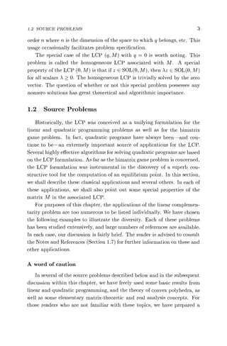
The Linear Complementarity Problem Classics In Applied Mathematics Richard W Cottle
The Linear Complementarity Problem Classics In Applied Mathematics Richard W Cottle


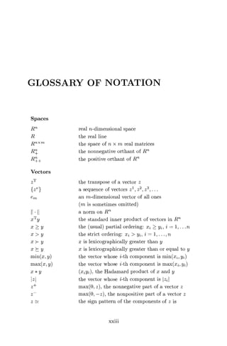
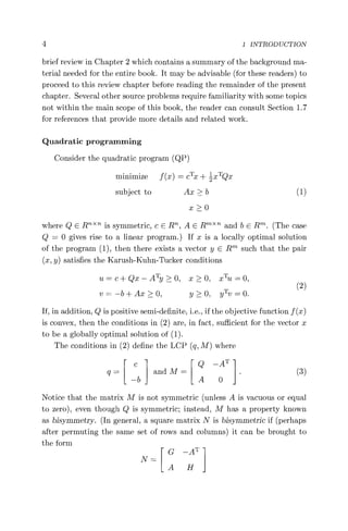
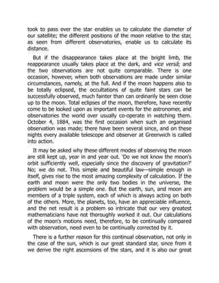
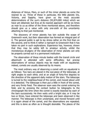
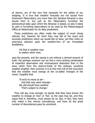
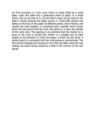
![GLOSSARY OF NOTATION
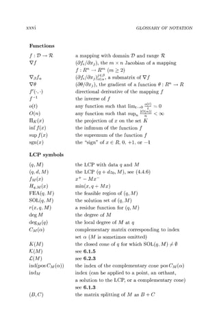
Sets
E element membership
not an element of
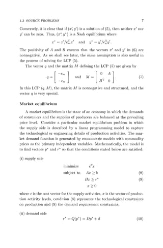
the empty set
C set inclusion
C proper set inclusion
U, n, x union, intersection, Cartesian product
Sl S2 the difference of sets Si and S2
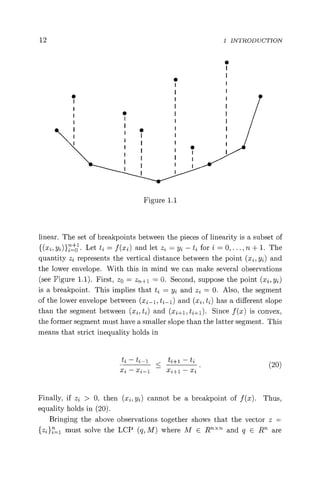
S1 O S2 (51 'S2) U (S2 Sl) _ (S1 U S2) (S1 n S2) ,
the symmetric difference of Sl and S2
Sl + Sz the (vector) sum of Sl and S2
the cardinality of a finite set S
SC the complement of a set S
dim S the dimension of a set S
bd S the (topological) boundary of a set S
cl S the (topological) closure of a set S
int S the topological interior of a set S
ri S the relative interior of a set S
rb S the relative boundary of a set S
S* the dual cone of S
O+S the set of recession directions of S
affn S the affine hull of S
cony S the convex hull of S
pos A the cone generated by the matrix A
[A] see 6.9.1
g(f) the graph of the function f
Sn-1 the unit sphere in Rn
£[x, y] the closed line segment between x and y
£(x, y) the open line segment between x and y
B(x, S) an (open) neighborhood of x with radius S
N(x) an (open) neighborhood of r
arg minx f (x) the set of x attaining the minimum of f (x)
arg maxi f (a) the set of x attaining the maximum of f (x)
[a, b] a closed interval in R
(a, b) an open interval in R
S the unit sphere
23 the closed unit ball
xxv](https://image.slidesharecdn.com/1271976-250526163136-bbc02400/85/The-Linear-Complementarity-Problem-Classics-In-Applied-Mathematics-Richard-W-Cottle-30-320.jpg)

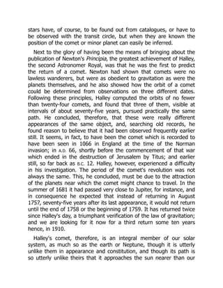
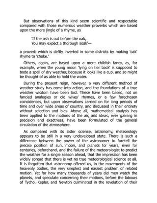
![timekeeper; not only in that of the moon, but also in the case of the
planets. Their places as computed need continually to be compared
with their places as observed, and the discordances, if any, inquired
into. The great triumph which resulted to science from following this
course—to pure science, since Uranus is too faint a planet to be any
help to the sailor in navigation—is well known. The observed
movements of Uranus proved not to be in accord with computation,
and from the discordances between calculation and observation
Adams and Leverrier were able to predicate the existence of a
hitherto unseen planet beyond—
'To see it, as Columbus saw America from Spain. Its
movements were felt by them trembling along the far-reaching
line of their analysis, with a certainty hardly inferior to that of
ocular demonstration.'[5]
The discovery of Neptune was not made at Greenwich, and Airy
has been often and bitterly attacked because he did not start on the
search for the predicted planet the moment Adams addressed his
first communication to him, and so allowed the French astronomer
to engross so much of the honour of the exploit. The controversy
has been argued over and over again, and we may be content to
leave it alone here. There is one point, however, which is hardly ever
mentioned, which must have had much effect in determining Airy's
conduct. In 1845, the year in which Adams sent his provisional
elements of the unseen disturbing planet to Airy, the largest
telescope available for the search at Greenwich was an equatorial of
only six and three-quarter inches aperture, provided with small and
insufficient circles for determining positions, and housed in a very
small and inconvenient dome; whilst at Cambridge, within a mile or
so of Adams' own college, was the 'Northumberland' equatorial, of
nearly twelve inches aperture, under the charge of the University
Professor of Astronomy, Professor Challis, and which was then much
the largest, best mounted and housed equatorial in the entire
country. The 'Northumberland' had been begun from Airy's designs
and under his own superintendence, when he was Professor of](https://image.slidesharecdn.com/1271976-250526163136-bbc02400/85/The-Linear-Complementarity-Problem-Classics-In-Applied-Mathematics-Richard-W-Cottle-61-320.jpg)


![[W]-REFERENCIA-Paul Waltman (Auth.) - A Second Course in Elementary Different...](https://cdn.slidesharecdn.com/ss_thumbnails/w-referencia-paulwaltmanauth-230516025940-c93e36a9-thumbnail.jpg?width=640&height=640&fit=bounds)


