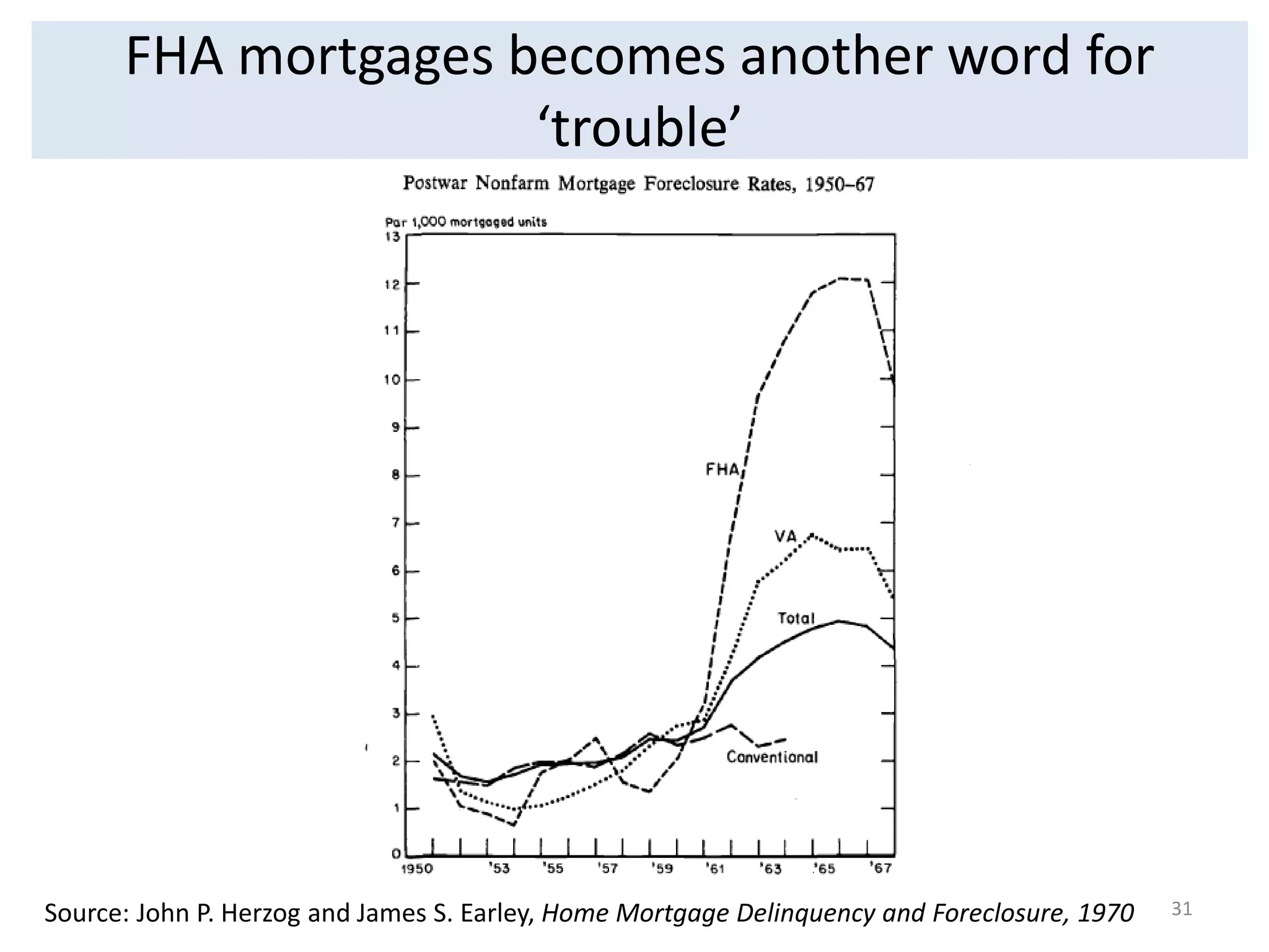
Download to read offline


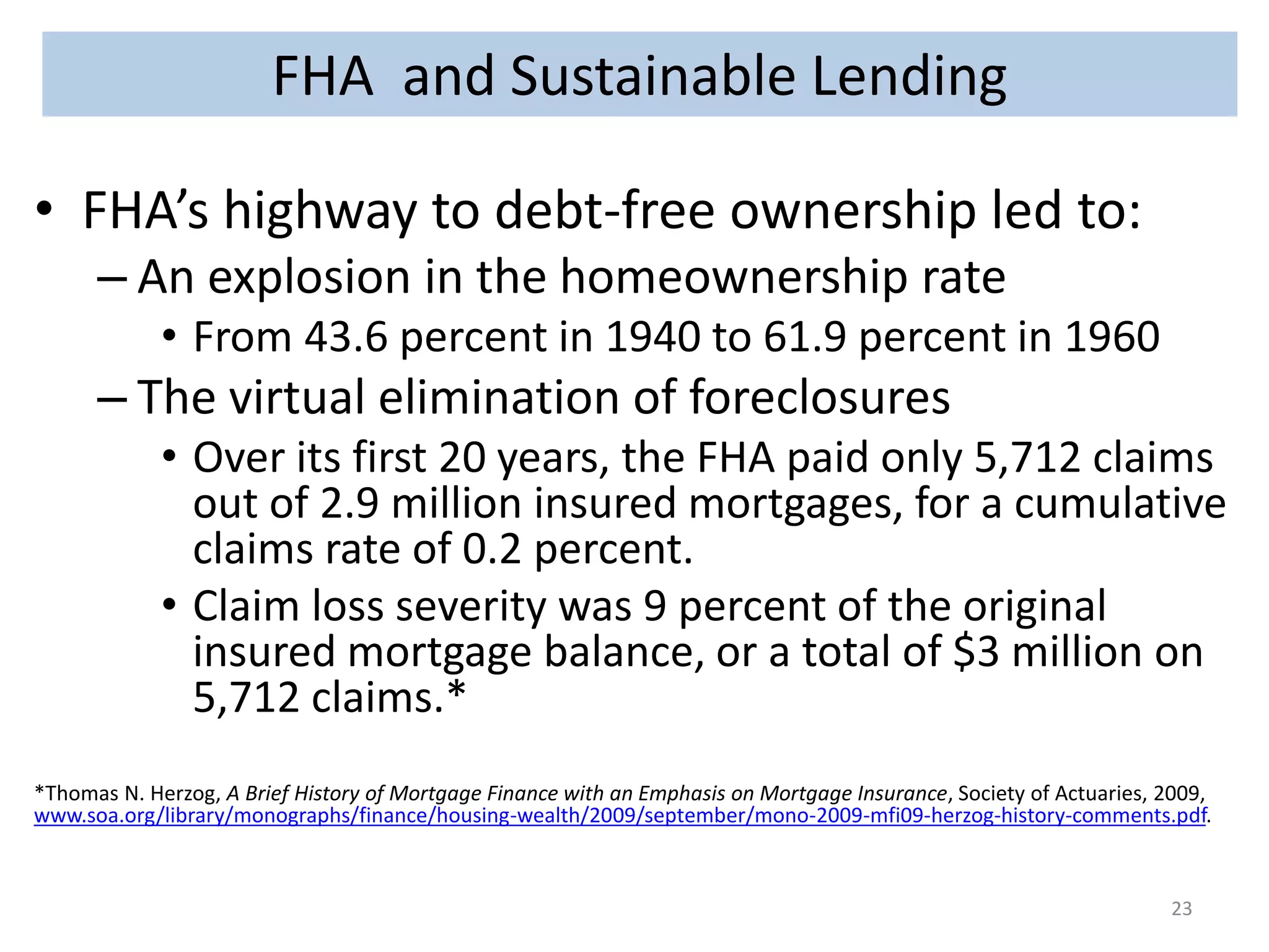
![FHA and Sustainable Lending
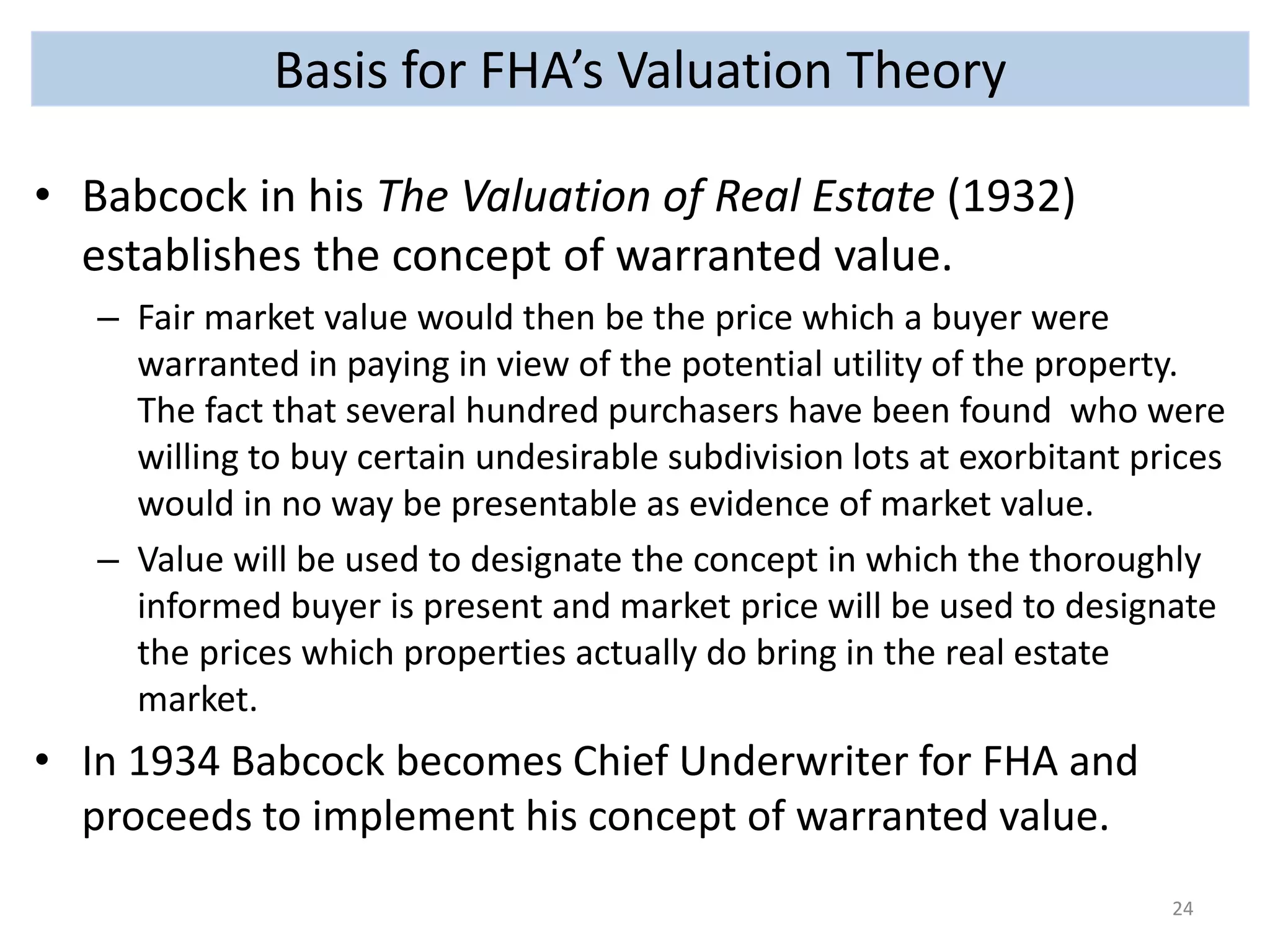
• 1935: “‘Mortgage’ was just another word for trouble—an epitaph
on the tombstone of their aspirations for home ownership.”*
– Replaces loose and dangerous lending practices that had made foreclosures
commonplace with “a straight, broad highway to debt-free ownership.”*
• “[s]uccessful mortgage lending must be predicated upon a measurement of risk
factors in mortgage investment. Mortgage risk comes into existence in the
moment mortgage funds are disbursed to a borrower. The risk continues until
there has been a complete recapture of the money which has been lent. This risk
is greater in some loans than in others. It differs from time to time for each loan.
The best we can hope to do is establish a method by means of which to estimate
the degree of risk at the time the loan is submitted. If the measurement of risk
indicates hazards which are too great, the institution must necessarily refuse to
make the loan. In other cases it is highly important that the institution
determine not only that it is willing to make the loan but the intrinsic quality of
the loan as a portion of its mortgage portfolio.” Frederick M Babcock, FHA’s first
chief underwriter
– Sound lending practices include:
• A sizable down payments (a minimum of 20%) and a maximum 20-year term;
• Solid borrower credit histories and solid appraisals;
• Ability to pay (imposed on FHA by the1934 National Housing Act): proper
income documentation and sufficient income to make regular payments
(includes review of a borrower’s monthly expenses and residual income);
• Fully amortized loan with a ban on second mortgages.
* Federal Housing Administration, “How to Have the Home You Want,” 1936.
21](https://image.slidesharecdn.com/pinto-devolutionluncheonpresentationataeiconference-140925132330-phpapp01/75/The-devolution-of-appraisal-and-underwriting-theory-and-practice-21-2048.jpg)

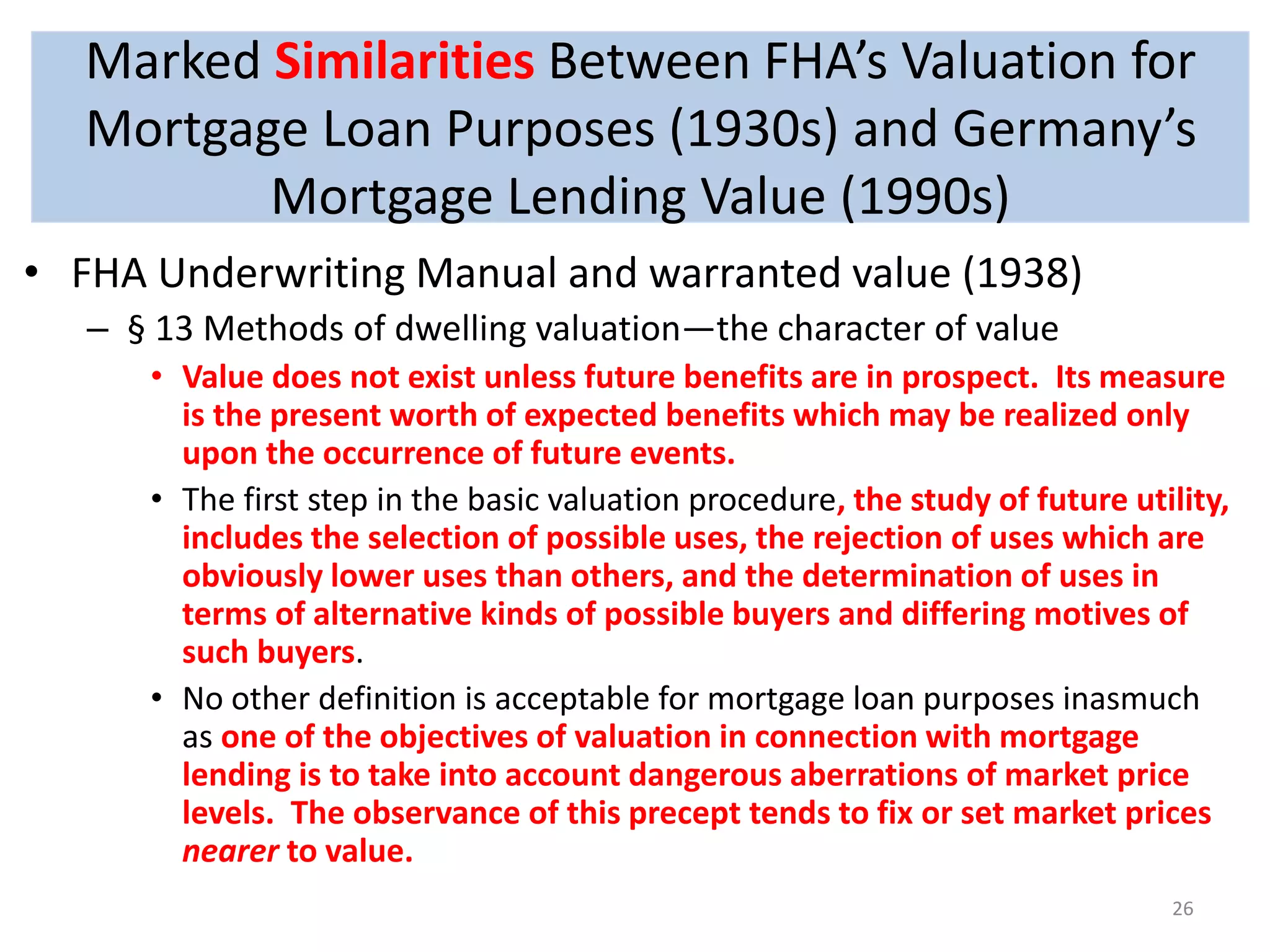
![Marked Similarities Between FHA’s Valuation for
Mortgage Loan Purposes (1930s) and Germany’s
Mortgage Lending Value (1990s)
• FHA Underwriting Manual and warranted value (1938)
– § 13 Methods of dwelling valuation—the character of value
• The word “value” refers to the price which a purchaser is warranted in
paying for a property for continued use or a long-term investment.
• The value to be estimated, therefore, is the probable price which typical
buyers are warranted in paying.
• This valuation is sometimes hypothetical in character, especially under
market conditions where abnormalities in price levels indicate the
presence of serious quantitative differentials the two value concepts
[warranted value and available market price].
• Marked differences between “available market prices” and “values” will
be evident under both boom and depression conditions of market.
• Attention is directed to the fact that speculative elements cannot be
considered as enhancing the security of residential loans. On the
contrary, such elements enhance the risk of loss to mortgagees who
permit them to creep into the valuations of properties upon which they
make loans.
25](https://image.slidesharecdn.com/pinto-devolutionluncheonpresentationataeiconference-140925132330-phpapp01/75/The-devolution-of-appraisal-and-underwriting-theory-and-practice-25-2048.jpg)

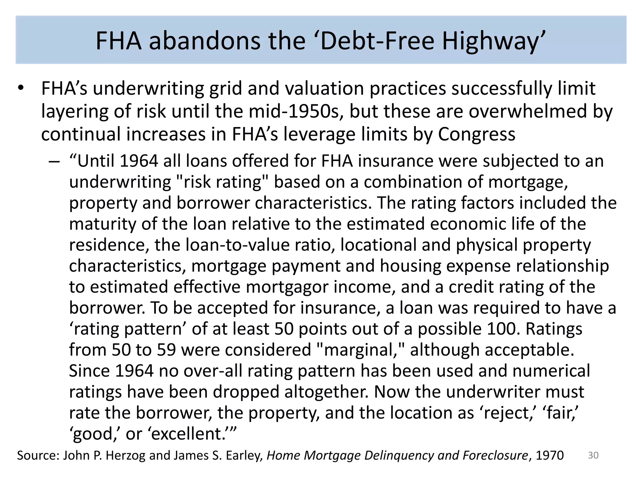
![1930s to Today – Policy Pressures to Increase All
Forms of Leverage
• Late-1930s on: Congress raises FHA leverage limits
– FHA’s underwriting grid and valuation practices limit layering of risk for 20
years
• 1992 and on: Congress places Fannie and Freddie in competition
with FHA and private subprime
• The result is a ‘curious’ policy whereby low income home buyers
with volatile incomes are encouraged to buy homes in areas with
volatile prices using high leverage
• Policies based on a view that “[o]ne unique aspect of
homeownership is that it is one of the few leveraged
investments available to households with little wealth,
enabling homeowners with very little equity in their homes to
benefit from appreciation in the overall home value.”1
1Herbert and Belsky, 2008, The Homeownership Experience of Low-Income and Minority Households: A Review
and Synthesis of the Literature, Cityscape: A Journal of Policy Development and Research
• T
29](https://image.slidesharecdn.com/pinto-devolutionluncheonpresentationataeiconference-140925132330-phpapp01/75/The-devolution-of-appraisal-and-underwriting-theory-and-practice-29-2048.jpg)


The document discusses the evolution of appraisal and underwriting practices in the housing market, highlighting the volatility in home prices and the impact of excessive leverage on wealth building. It emphasizes the need for sound lending practices to mitigate risks associated with mortgage debt, particularly during economic downturns. Key historical insights are drawn from past housing policies and their results on homeownership rates and foreclosure elimination.


![6 10 10 Revised Marcs Published Work Presentation (2)[1]](https://cdn.slidesharecdn.com/ss_thumbnails/61010revisedmarcspublishedworkpresentation21-12794895695744-phpapp02-thumbnail.jpg?width=640&height=640&fit=bounds)


