Particle sworm

1. Review of Evolutionary
Multimodal Multiobjective
Optimization
Hassan Raza
19i-1611

2. Problem Statement

Multimodal multiobjective optimization has been
investigated in the evolutionary computation
community since 2005

However, it is difficult to survey existing studies
in this field because they have been
independently conducted and do not explicitly
use the term “multimodal multiobjective
optimization.”

3. Solution

To address this issue, this paper reviews the
existing studies of evolutionary multimodal
multiobjective optimization, including studies
published under names that are different from
multimodal multiobjective optimization.

4. Introduction

A multiobjective evolutionary algorithm (MOEA) is an
efficient optimizer for a multiobjective optimization
problem (MOP)

MOEAs aim to find a nondominated solution set that
approximates the Pareto front in the objective space.

The set of nondominated solutions found by an MOEA is
usually used in an a posteriori decision-making process

A decision maker selects a final solution from the
solution set according to his/her preference.

5. Introduction

Since the quality of a solution set is usually
evaluated in the objective space, the distribution of
solutions in the solution space has not received
much attention in the evolutionary multiobjective
optimization (EMO) community.

However, the decision maker may want to
compare the final solution to other dissimilar
solutions that have an equivalent quality or a
slightly inferior quality.

6. Inroduction
 four solutions xa
, x b
, x c
, and x d
are far from
each other in the solution space but close to
each other in the objective space.

7. Inroduction

This kind of situation can be found in a number
of real-world problems, including functional brain
imaging problems, diesel engine design
problems, distillation plant layout problems,
rocket engine design problems, and game map
generation problems

8. Inroduction

If multiple diverse solutions with similar objective
vectors like xa
, xb
, xc
, and xd
are obtained, the decision
maker can select the final solution according to her/his
preference in the solution space.
 For example,if xa
becomes unavailable for some
reason(e.g material shortages, mechanical failures,
traffic accidents, and law revisions), the decision maker
can select a substitute from x b
, x c
, and x d
.

9. Introduction

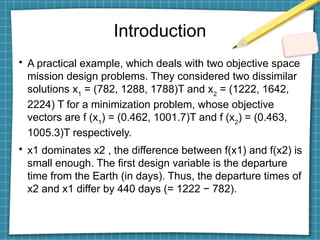
A practical example, which deals with two objective space
mission design problems. They considered two dissimilar
solutions x1
= (782, 1288, 1788)T and x2
= (1222, 1642,
2224) T for a minimization problem, whose objective
vectors are f (x1
) = (0.462, 1001.7)T and f (x2
) = (0.463,
1005.3)T respectively.

x1 dominates x2 , the difference between f(x1) and f(x2) is
small enough. The first design variable is the departure
time from the Earth (in days). Thus, the departure times of
x2 and x1 differ by 440 days (= 1222 − 782).

10. Introduction

multiple solutions with almost equivalent quality
support a reliable decision-making process.

If these solutions have a large diversity in the
solution space, they can provide insightful
information for engineering design

A multimodal MOP (MMOP) involves finding all
solutions that are equivalent to Pareto optimal
solutions

11. MOP& MMOP

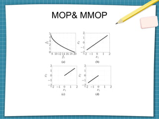
12. MOP& MMOP

Since most MOEAs (e.g., NSGA-II and SPEA2)
do not have mechanisms to maintain the
solution space diversity, it is expected that they
do not work well for MMOPs.

Thus, multimodal multiobjective evolutionary
algorithms (MMEAs) that handle the solution
space diversity are necessary for MMOPs.

13. Definition of MOPs

A continuous MOP involves finding a solution x S R
∈ ⊆ D
that
minimizes a given objective function vector f : S → R M
. Here, S
is the D-dimensional solution space, and R M
is the M-
dimensional objective space.

A solution x1 is said to dominate x2 iff fi(x1) ≤ fi(x2) for all i {1,
∈
. . . , M} and fi(x1) < fi(x2) for at least one index i. If x is not
∗
dominated by any other solutions, it is called a Pareto optimal
solution. The set of all x is the Pareto optimal solution set.
∗

set of all f (x ) is the Pareto front. The goal of MOPs is to find
∗
a nondominated solution set that approximates the Pareto front
in the objective space.

14. Definition of MMOPs

An MMOP involves finding all solutions that are equivalent to
Pareto optimal solutions.

Two different solutions x1 and x2 are said to be equivalent iff f(x1) −
f(x2) ≤ δ, where a is an arbitrary norm of a, and δ is a non-negative
threshold value given by the decision maker.

If δ =0, the MMOP should find all equivalent Pareto optimal
solutions.

If δ > 0, the MMOP should find all equivalent Pareto optimal
solutions and dominated solutions with acceptable quality.

The main advantage of this definition is that the decision maker can
adjust the goal of the MMOP by changing the δ value.

15. MMEAs

MMEAs need the following three abilities:

1) the ability to find solutions with high quality

2) the ability to find diverse solutions in the
objective space

3) the ability to find diverse solutions in the
solution space.

16. MMEAs

This paper describes 12 dominance-based
MMEAs, 3 decomposition-based MMEAs, 2 set-
based MMEAs, and a post-processing
approach.

17. Pareto Dominance-Based MMEAs

The most representative MMEA is Omni-optimizer which
is an NSGA-II-based generic optimizer applicable to
various types of problems. The differences between
Omni-optimizer and NSGA-II are fourfold:

the Latin hypercube sampling-based population
initialization.

the so-called restricted mating selection.

e-dominance-based nondominated sorting.

the alternative crowding distance.

18. Pareto Dominance-Based MMEAs
 In the restricted mating selection, an individual xa
is randomly selected
from the population.
 Then, xa
and its nearest neighbor xb
in the solution space are compared
based on their non-domination levels and crowding distance values.

The winner among both is selected as a parent.

The crowding distance measure in Omni-optimizer takes into account
both the objective and solution spaces.

Omni-optimizer finds more diverse solutions than NSGA-II due to
alternative crowded distance.

Others DNEA,DN-NSGA-II,DBSCAN,SPEA2+

19. Decomposition-Based MMEAs

A three-phase multistart method is proposed. First, (1, λ)- ES is carried out
on each M objective functions K times to obtain M×K best-so-far solutions.

Then, an unsupervised clustering method is applied to the M × K solutions
to detect the number of equivalent Pareto optimal solution subsets s.

Finally, s runs of (1, λ)-ES are performed on each N single-objective
subproblem decomposed by the Tchebycheff function.

The initial individual of each run is determined in a chained manner. The
best solution found in the jth subproblem becomes an initial individual of (1,
λ)-ES for the j + 1st subproblem (j {1, . . . , N − 1}). It is expected that s
∈
equivalent solutions are found for each N decomposed subproblems.

20. Decomposition-Based MMEAs

Two variants of MOEA/D for MMOPs are proposed.

MOEA/D decomposes an M-objective problem into N single-objective
subproblems using a set of weight vectors, assigning a single individual to
each subproblem.

Then, MOEA/D simultaneously evolves the N individuals. Two methods
assign one or more individuals to each subproblem to handle the equivalency.

The MOEA/D algorithm presented in 1st assigns K individuals to each
subproblem. The selection is conducted based on a fitness value combining
the PBI function value and two distance values in the solution space. K
dissimilar individuals are likely to be assigned to each subproblem. The main
drawback is the difficulty in setting a proper value for K, because it is problem
dependent.

21. Decomposition-Based MMEAs

2
nd
does not need such a parameter but
requires a relative neighborhood size L. For
each iteration, a child u is assigned to the jth
subproblem whose weight vector is closest to
f(u), with respect to the perpendicular distance.

22. Set-Based MMEAs

DIOP is a set-based MMEA that can maintain dominated solutions in
the population. In the set-based optimization framework, a single
solution in the upper level represents a set of solutions in the lower
level (i.e., a problem). DIOP simultaneously evolves an archive A
and a target population T.

While A approximates only the Pareto front and is not shown to the
decision maker, T obtains diverse solutions with acceptable quality
by maximizing the following G indicator:G(T)=wobj
Dobj
(T)+wsol
D sol
(T).
Here, wobj
+ wsol
= 1.
 Dobj
is a performance indicator in the objective space, and Dsol
is a
diversity measure in the solution space.

23. Set-Based MMEAs

Another set-based MMEA unlike DIOP,

the proposed method evolves only a single
population. Whereas DIOP maximizes the
weighted sum of values of Dobj
and Dsol
, the
proposed method treats Dobj
and Dsol
as meta
two-objective functions. NSGA-II is used to
simultaneously maximize Dobj
and Dsol

24. Post-Processing Approach

it is not always necessary to locate all Pareto optimal solutions.

Suppose that a set of nondominated solutions A has already been obtained by an
MOEA (e.g., NSGA-II) but not an MMEA (e.g., Omni-optimizer). After the decision
maker has selected the final solution xfinal
from A according to her/his preference in the
objective space, it is sufficient to search solutions whose objective vectors are
equivalent to f (xfinal
).

A post-processing approach to handle this problem. First, the proposed approach
formulates a meta constrained two-objective minimization problem where

The meta objective functions f 1 meta and f 2 meta represent the distance between x
and x final in the objective and solution spaces. Thus, smaller f 1 meta (x) and f 2 meta
(x) indicate that x is similar to x final in the objective space and far from x final in the
solution space, respectively.

The constraint g meta with θ > 0 prevents f 2 meta (x) from becoming an infinitely small
value in unbounded problems.

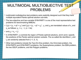
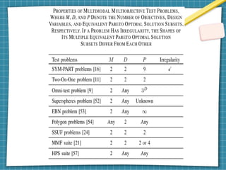
26. MULTIMODAL MULTIOBJECTIVE TEST
PROBLEMS

multimodal multiobjective test problems were explicitly designed such that they have
multiple equivalent Pareto optimal solution sub-sets.

The two-objective and two-variable SYM-PART1 is one of the most representative test
problems for benchmarking MMEAs:
 f1
(y) = (y1
+ a)2
+ y2
2
and f2
(y) = (y1
− a)2
+ y2
2
. y1
and y2
are translated values of x1
and
x2
as follows: y1
= x1
− t1
(c + 2a)
 and y2
= x2
− t2
b
.

In SYM-PART1, a controls the region of Pareto optimal solutions, and b and c specify
the positions of the Pareto optimal solution subsets. The so-called tile identifiers t1
and
t2
are randomly selected from {−1, 0, 1}.

Other test problems include the Two-On-One problem, the Omni-test problem, the
SYM-PART2 and SYM-PART3 problems, the Superspheres problem, the EBN problem,
the two SSUF problems, and the Polygon problems.

27. TEST PROBLEMS

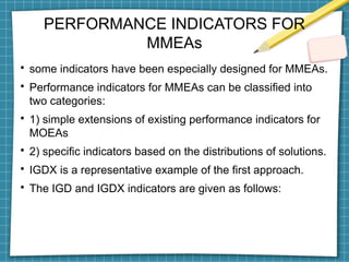
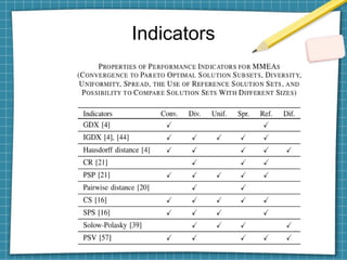
28. PERFORMANCE INDICATORS FOR
MMEAs

some indicators have been especially designed for MMEAs.

Performance indicators for MMEAs can be classified into
two categories:

1) simple extensions of existing performance indicators for
MOEAs

2) specific indicators based on the distributions of solutions.

IGDX is a representative example of the first approach.

The IGD and IGDX indicators are given as follows:

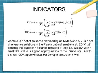
29. INDICATORS

where A is a set of solutions obtained by an MMEA and A is a set
∗
of reference solutions in the Pareto optimal solution set. ED(x1,x2)
denotes the Euclidean distance between x1 and x2. While A with a
small IGD value is a good approximation of the Pareto front, A with
a small IGDX approximates Pareto optimal solutions well

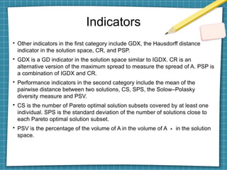
30. Indicators

Other indicators in the first category include GDX, the Hausdorff distance
indicator in the solution space, CR, and PSP.

GDX is a GD indicator in the solution space similar to IGDX. CR is an
alternative version of the maximum spread to measure the spread of A. PSP is
a combination of IGDX and CR.

Performance indicators in the second category include the mean of the
pairwise distance between two solutions, CS, SPS, the Solow–Polasky
diversity measure and PSV.

CS is the number of Pareto optimal solution subsets covered by at least one
individual. SPS is the standard deviation of the number of solutions close to
each Pareto optimal solution subset.

PSV is the percentage of the volume of A in the volume of A in the solution
∗
space.

31. Indicators