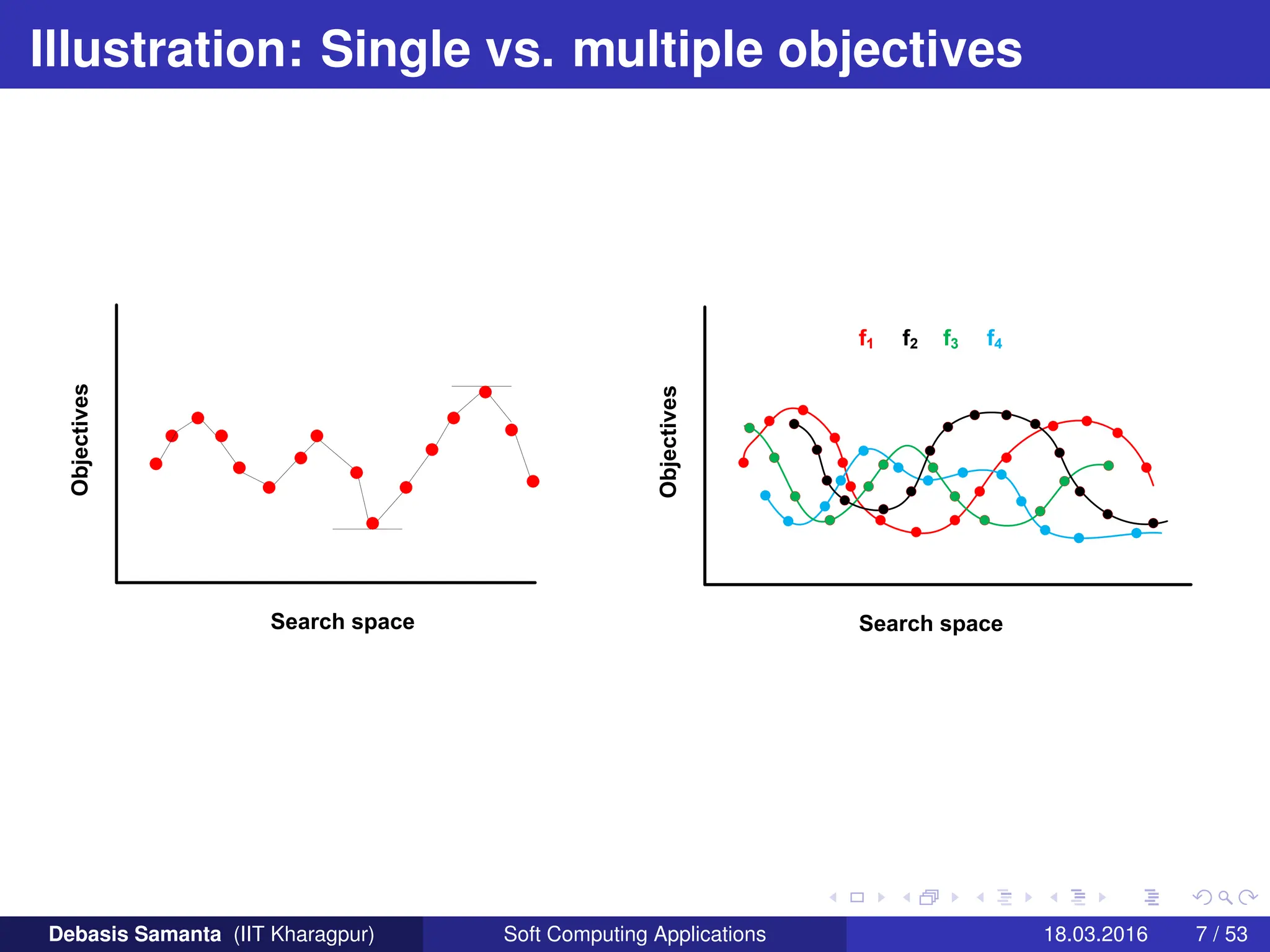
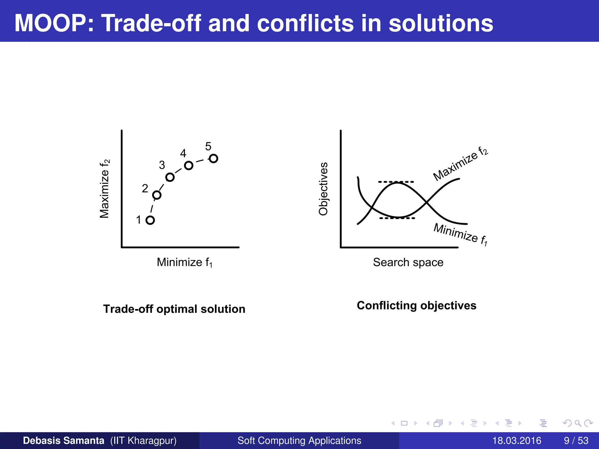
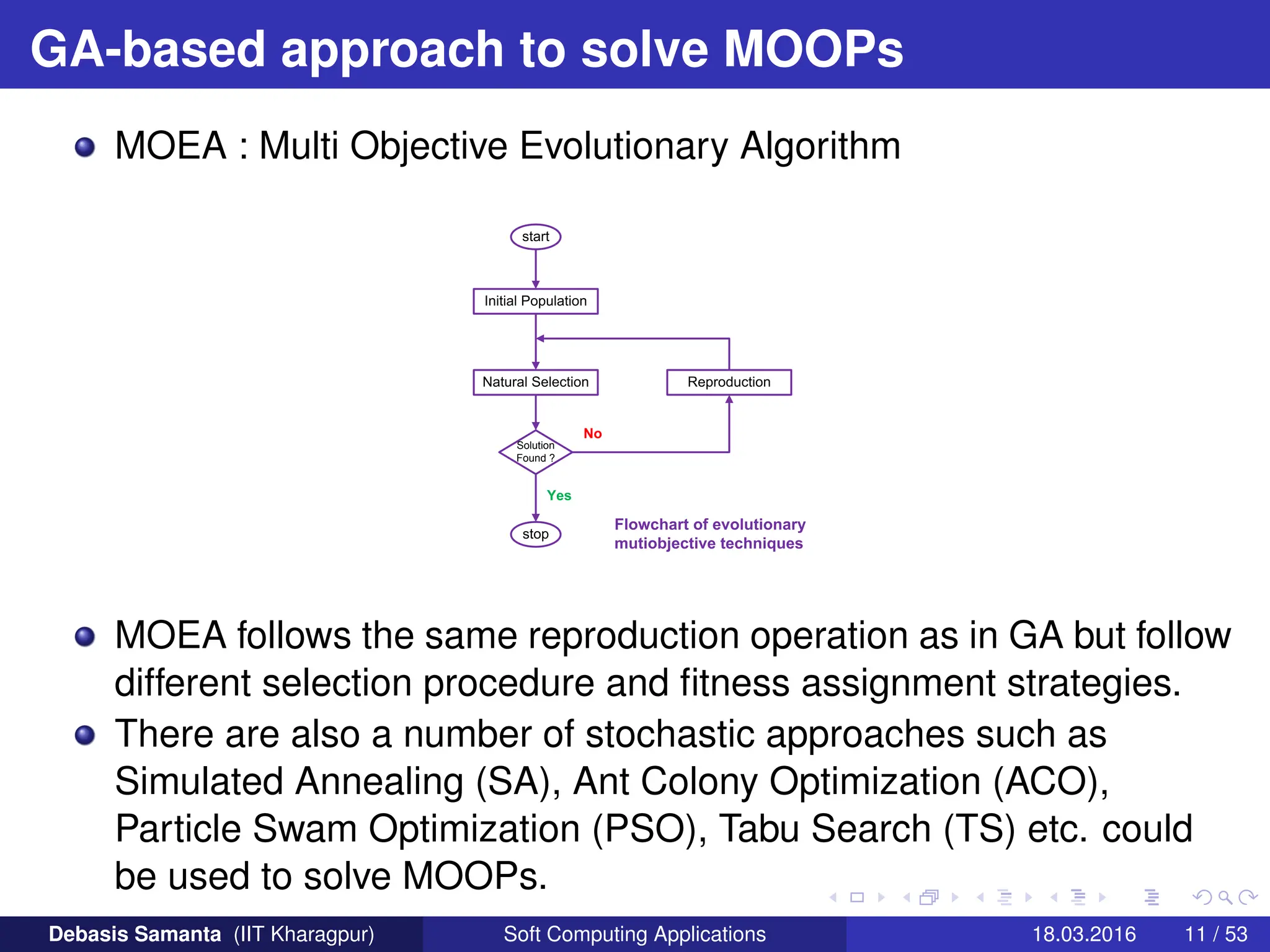
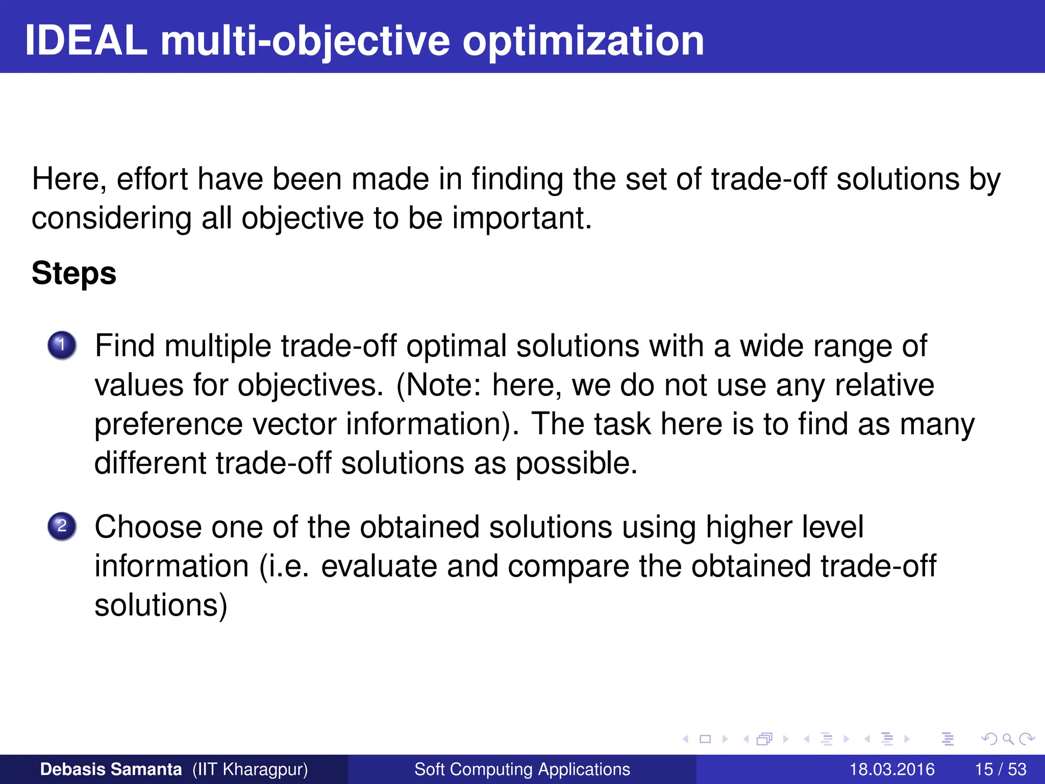
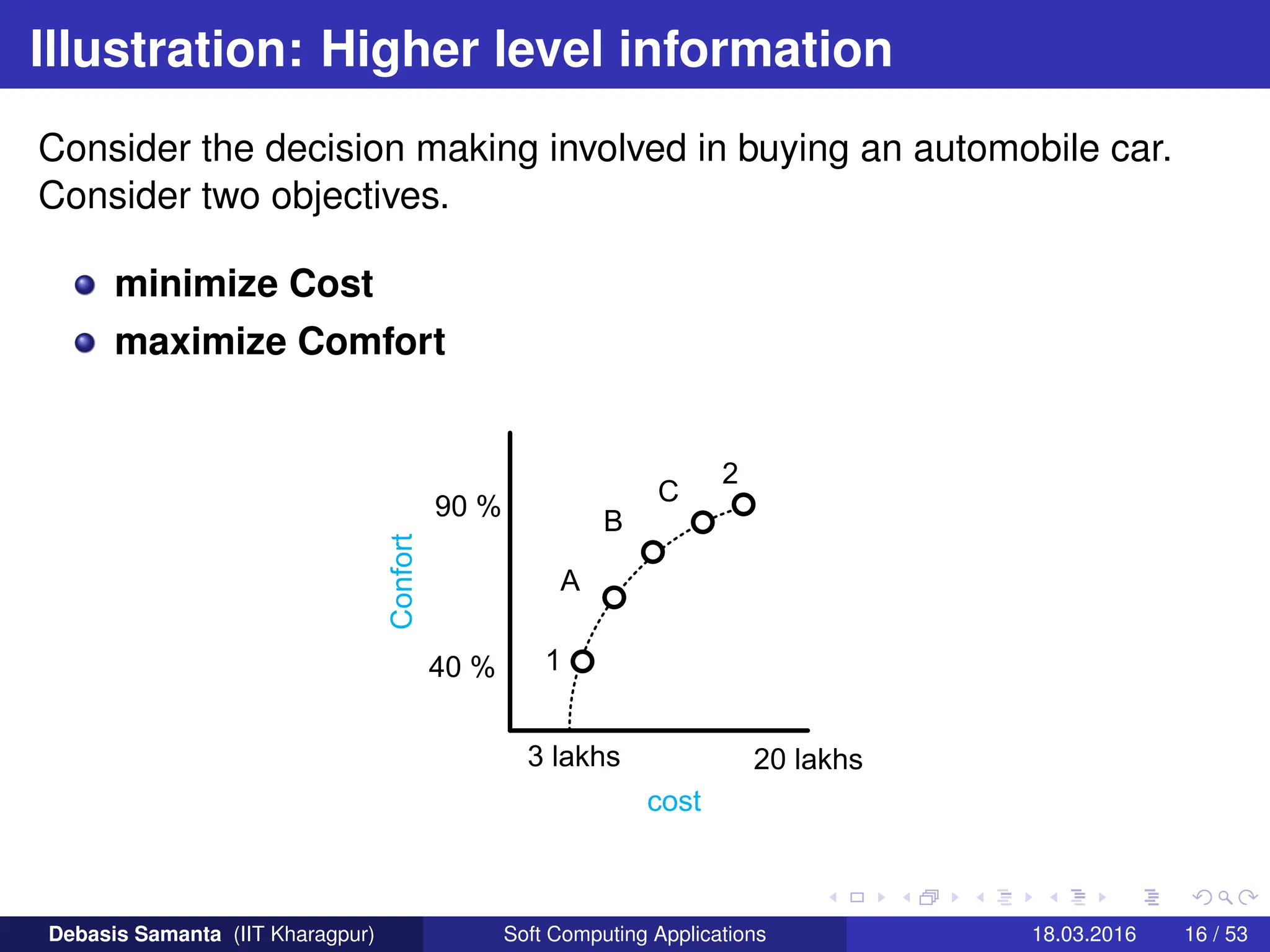
New very very interesting Ppt best notesnew.pdf

Multi-Objective Optimization: Introduction
Debasis Samanta
Indian Institute of Technology Kharagpur
dsamanta@iitkgp.ac.in
18.03.2016
Debasis Samanta (IIT Kharagpur) Soft Computing Applications 18.03.2016 1 / 53

Multiobjective optimization problem: MOOP
There are three components in any optimization problem:
F: Objectives
minimize (maximize) fi(x1, x2, · · · , xn), i = 1, 2, · · · , m
S: Constraints
Subject to
gj(x1, x2, · · · , xn), ROPj Cj, j = 1, 2, · · · , l
V: Design variables
xk ROPk dk , k = 1, 2, · · · , n
Note :
1 For a multi-objective optimization problem (MOOP), m ≥ 2
2 Objective functions can be either minimization, maximization or
both.

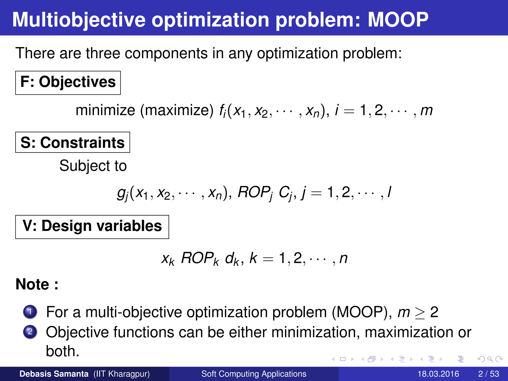
A formal specification of MOOP
Let us consider, without loss of generality, a multi-objective
optimization problem with n decision variables and m objective
functions
Minimize y = f(x) = [y1 ∈ f1(x), y2 ∈ f2(x), · · · , yk ∈ fm(x)]
where
x = [x1, x2, · · · , xn] ∈ X
y = [y1, y2, · · · , yn] ∈ Y
Here :
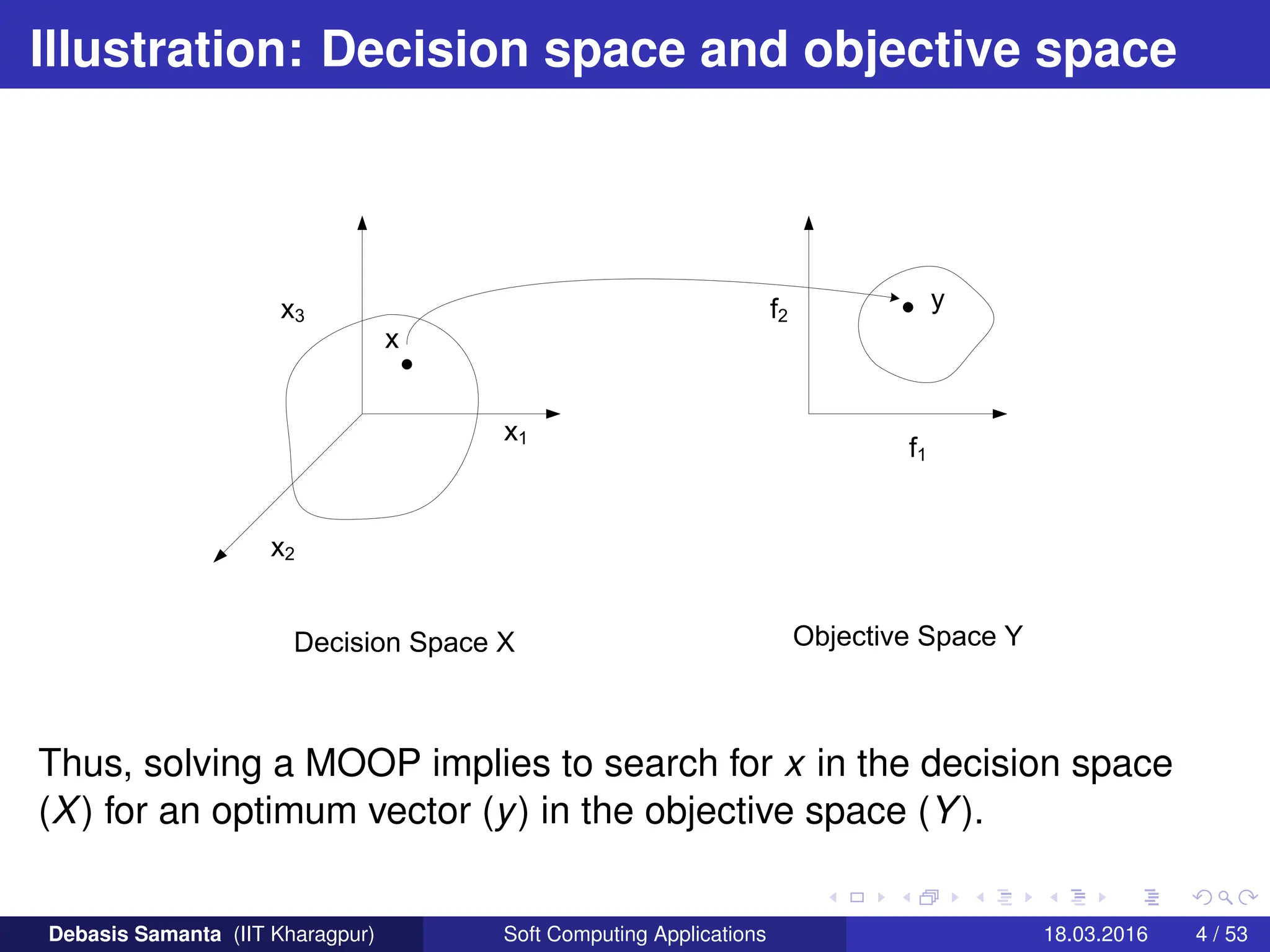
x is called decision vector
y is called an objective vector
X is called a decision space
Y is called an objective space

Illustration: Decision space and objective space
3
1
2
2
1
Thus, solving a MOOP implies to search for x in the decision space
(X) for an optimum vector (y) in the objective space (Y).

A formal specification of MOOP (contd...)
In other words,
1 We wish to determine X̄ ∈ X (called feasible region in X) and any
point x̄ ∈ X̄ (which satisfy all the constraints in MOOP) is called
feasible solution.
2 Also, we wish to determine from among the set X̄, a particular
solution x̄∗ that yield the optimum values of the objective functions.
Mathematically,
∀x̄ ∈ X̄ and ∃x̄∗ ∈ X̄ | fi(x̄∗) ≤ fi(x̄),
where ∀i ∈ [1, 2, · · · , m]
3 If this is the case, then we say that ¯
x∗ is a desirable solution.

Why solving a MOOP is an issue?
In a single-objective optimization problem, task is to find typically
one solution which optimizes the sole objective function
In contrast to single–objective optimization problem, in MOOP:
Cardinality of the optimal set is more than one, that is, there are
m ≥ 2 goals of optimization instead of one
There are m ≥ 2 different search points (possibly in different
decision spaces) corresponding to m objectives
Optimizing each objective individually not necessarily gives the
optimum solution.
Possible, only if objective functions are independent to their solution
spaces.

Illustration: Single vs. multiple objectives
Search space
Objectives
f1 f2 f3 f4
Search space
Objectives

Why solving an MOOP is an issue?
In fact, majority of the real-world MOOPs are with a set of trade-off
optimal solutions. A set of trade-off optimal solutions is also
popularly termed as Pareto optimal solutions
In a particular search point, one may be the best whereas other
may be the worst
Also, sometime MOOPs are with conflicting objectives
Thus, optimizing an objective means compromising other(s) and
vice-versa.

MOOP: Trade-off and conflicts in solutions
1
2
3
4
5
Maximize
f
2
Minimize f1
Trade-off optimal solution
Objectives
Search space
Conflicting objectives
Maximize f2
Minimize f1

Illustration: ideal solution vs. real solution
It is observed that in many real-life problems, we hardly have a
situation in which all the fi(x̄) have a minimum in X̄ at a common point
x̄∗.
This is particularly true when objective functions are conflicting in their
interests.
F1 (minimize)
F
2
(minimize)
F
2
(minimize)
F1 (minimize)
Ideal Situation Real Situation

GA-based approach to solve MOOPs
MOEA : Multi Objective Evolutionary Algorithm
Solution
Found ?
MOEA follows the same reproduction operation as in GA but follow
different selection procedure and fitness assignment strategies.
There are also a number of stochastic approaches such as
Simulated Annealing (SA), Ant Colony Optimization (ACO),
Particle Swam Optimization (PSO), Tabu Search (TS) etc. could
be used to solve MOOPs.

MOEA: GA-based approach to solve MOOP
There are two board approaches to solve MOOPs with MOEA
A priori approach (also called preference based approach)
A posteriori approach (does not require any prior knowledge)
Two major problems must be addressed when a GA is applied to
multi-objective optimization problems.
1 How to accomplish fitness assignment and selection in order to
guide the search toward the optimal solution set?
2 How to maintain a diverse population in order to prevent
premature convergence and achieve a well distributed trade-off
front?

Schematic of a priori MOEA approach
A MOOP problem
Minimize f1
Minimize f2
. . . . . . . . .
Minimize fm
Higher level
information
Estimate a
relative
importance
vector W =
{w1,w2 . . .wm}
Single-objective
optimization problem
Subject to S and V
GA to solve
the problem
Single Optimal
Solution
Subject to
constraint S
with design
variables V
1
m
i i
i
F w f

 


Schematic of a posteriori MOEA approach
A MOOP problem
Minimize f1
Minimize f2
. . . . . . . . .
Minimize fm
Ideal
Multiobjective
Optimizer
Multiple Pareto-
optimal
solutions
Higher level
Informaiton
Choose one
solution
Subject to
constraint S
with design
variables V

IDEAL multi-objective optimization
Here, effort have been made in finding the set of trade-off solutions by
considering all objective to be important.
Steps
1 Find multiple trade-off optimal solutions with a wide range of
values for objectives. (Note: here, we do not use any relative
preference vector information). The task here is to find as many
different trade-off solutions as possible.
2 Choose one of the obtained solutions using higher level
information (i.e. evaluate and compare the obtained trade-off
solutions)

Illustration: Higher level information
Consider the decision making involved in buying an automobile car.
Consider two objectives.
minimize Cost
maximize Comfort

Illustration: Higher level information
Here, solution 1 and 2 are two extreme cases.
Between these two extreme solutions, there exist many other
solutions, where trade-off between cost and comfort exist.
In this case, all such trade-off solutions are optimal solutions to a
multi-objective optimization problem.
Often, such trade-off solution provides a clear front on an
objective space plotted with the objective values.
This front is called Pareto-optimal front and all such trade-off
solutions are called Pareto-optimal solutions (after the name of
Vilfredo Pareto, 1986)

Choosing a solution with higher level information
Knowing the number of solutions that exist in the market with
different trade-offs between cost and comfort, which car does one
buy?
It involves many other considerations
total finance available to buy the car
fuel consumption
depreciation value
road condition
physical health of the passengers
social status
After sales service, vendor’s reputation, manufacturer’s past history
etc.

Formal specification of MOEA approach
In the next few slides, we shall discuss the above idea of solving
MOOPs more precisely. Before that, let us familiar to few more basic
definitions and terminologies.
1 Concept of domination
2 Properties of dominance relation
3 Pareto-optimization
4 Solutions with multiple-objectives

Solution with multiple objectives : Ideal objective
vector
For each of the M-th conflicting objectives, there exist one different
optimal solution. An objective vector constructed with these individual
optimal objective values constitute the ideal objective vector.
Definition 1: Ideal objective vector
Without any loss of generality, suppose the MOOP is defined as
Minimize fm(x), m = 1, 2, · · · , M
Subject to X ∈ S, where S denotes the search space.
and
f∗
m denotes the minimum solution for the m-th objective functions, then
the ideal objective vector can be defined as
Z∗ = f∗ = [f∗
1 , f∗
2 , · · · , f∗
M]

Ideal objective vector : Physical interpretation
(A) Ideal objective vector
(B) A good solution vector should
be as close to ideal solution vector
f1
f2
Z*
1
Z*
2
Z*
Z*
f2
f1
Z*

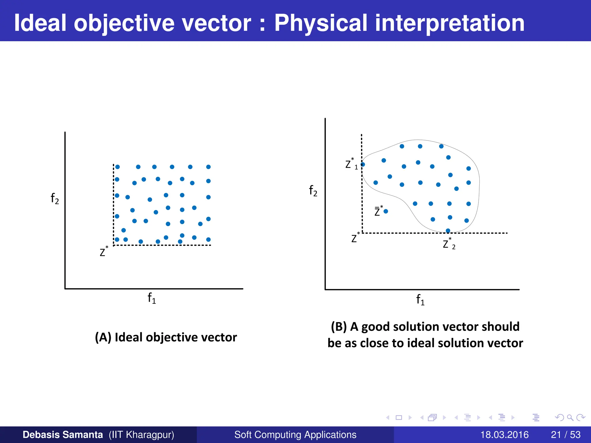
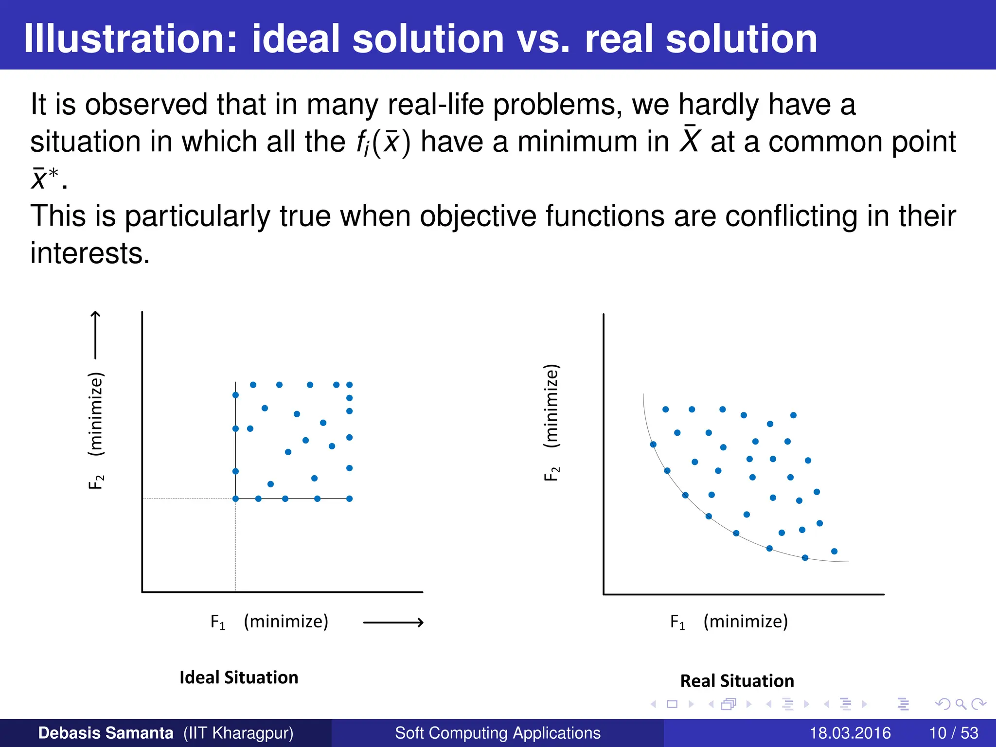
Ideal objective vector : Physical interpretation
Let us consider a MOOP with two objective functions f1 and f2 where
both are to be minimized.
If z∗ = f∗ = [f∗
1 , f∗
2 ] then both f1 and f2 are minimum at x∗ ∈ S.
(That is, there is a feasible solution when the minimum solutions to
both the objective functions are identical).
In general, the ideal objective vector z∗ corresponds to a
non-existent solution (this is because the minimum solution for
each objective function need not be the same solution).
If there exist an ideal objective vector, then the objectives are
non-conflicting with each other and the minimum solution to any
objective function would be the only optimal solution to the MOOP.
Although, an ideal objective vector is usually non-existing, it is
useful in the sense that any solution closer to the ideal objective
vector are better. (In other words, it provides a knowledge on the
lower bound on each objective function to normalize objective
values within a common range).

Solution with multiple objectives : Utopian
objective vector
Utopian objective vector corresponding to a solution which has an
objective value strictly better than (and not equal to) that of any
solution in search space.
f1
f2
Z*
Z**
Utopian objective vector
Ideal objective vector

Solution with multiple objectives : Utopian
objective vector
The Utopian objective vector can be formally defined as follows.
Definition 2 : Utopian objective vector
A Utopian objective vector z∗∗ has each of its component marginally
smaller than that of the ideal objective vector, that is
z∗∗
i = z∗
i − ∈i with ∈i> 0 for all i = 1, 2, · · · , M
Note :
Like the ideal objective vector, the Utopian objective vector also
represents a non-existent solution.

Solution with multiple objectives : Nadir objective
vector
The ideal objective vector represents the lower bound of each
objective in the entire feasible search space. In contrast to this, the
Nadir objective vector, denoted as znadir , represents the upper bound
of each objective in the entire Pareto-optimal set (note: not in the
entire search space).
1
2
Z*
Z1
*
Z2
*
Znadir
(f1
max
,f2
max
)

Solution with multiple objectives : Nadir objective
vector
Note :
znadir is the upper bound with respect to Pareto optimal set. Whereas,
a vector of objective W found by using the worst feasible function
values fmax
i in the entire search space.

Usefulness of Nadir objective vector
In order to normalize each objective in the entire range of
Pareto-optimal region, the knowledge of Nadir and ideal objective
vectors can be used as follows.
¯
fi =
fi −z∗
i
znadir
i
−z∗
i

Concept of domination
Notation
Suppose, f1, f2, · · · , fM are the objective functions
xi and xj are any two solutions
The operator between two solutions xi and xj as xi xj to
denote that solution xi is better than the solution xj on a particular
objective.
Alternatively, xi xj for a particular objective implies that solution
xi is worst than the solution xj on this objective.
Note :
If an objective function is to be minimized, the operator would mean
the ”” (less than operator), whereas if the objective function is to be
maximized, the operator would mean the ”” (greater than operator).

Concept of domination
Definition 3 : Domination
A solution xi is said to dominate the other solution xj if both condition I
and II are true.
Condition : I
The solution xi is no worse than xj in all objectives. That is
fk (xi) 7 fk (xj) for all k = 1, 2, · · · , M
Condition : II
The solution xi is strictly better than xj in at least one objective. That is
fk̄ (xi) fk̄ (xj) for at least one k̄ ∈ {1, 2, · · · , M}

Illustration 1
Consider that f1 and f2 are two objectives to be minimized.
f1
f2
x1
x2
x3
Minimize f1
Minimize f2
x1 ≤ x2
x1 ≤ x3
x2 ≤ x3
but x3 ≤ x1
as well as x3 ≤ x2

Illustration 2
f1
f2
x1
x2
x3 Minimize f1
Maximize f2
x1 ≤ x2 or x2 ≤ x1
x1 ≤ x3 or x3 ≤ x1
x2 ≤ x3 or x3 ≤ x2
?
?
?

Points to be noted
Note :
If either of the condition I and II is violated then the solution xi
does not dominate the solution xj.
If xi dominates the solution xj (it is also mathematically denoted as
xi ≤ xj.
The domination also alternatively can be stated in any of the
following ways.
xj is dominated by xi
xi is non-dominated by xj
xi is non-inferior to xj

Illustration 3
f1 maximize
1
2
3
4
5
2
4
5
3
1
2 6 10 14 18
f
2
minimize
Here, 1 dominates 2, 5 dominates 1 etc.

Properties of dominance relation
Definition 3 defines the dominance relation between any two
solutions.
This dominance relation satisfies four binary relation properties.
Reflexive :
The dominance relation is NOT reflexive.
Any solution x does not dominate itself.
Condition II of definition 3 does not allow the reflexive property to
be satisfied.
Symmetric :
The dominance relation also NOT symmetric
x y does not imply y x.

Antisymmetric :
Dominance relation can not be antisymmetric
Transitive :
The dominance relation is TRANSITIVE
If x y and y z, then x z.

Note :
1 An interesting property that dominance relation possesses is : If
solution x does not dominate solution y, this does not imply that y
dominates x.
2 In order for a binary relation to qualify as an ordering relation, it
must be at least transitive. Hence, dominance relation qualifies as
an ordering relation.
3 A relation is called partially ordered set, if it is reflexive,
antisymmetric and transitive. Since dominance relation is NOT
REFLEXIVE, NOT ANTISYMMETRIC, it is NOT a PARTIALLY
ORDER RELATION
4 Since, the dominance relation is not reflexive, it is a STRICT
PARTIAL ORDER.

Pareto optimality
f1 maximize
1
2
3
4
5
2
4
5
3
1
2 6 10 14 18
f
2
minimize
Non-dominated front

Pareto optimality
Consider solution 3 and 5.
Solution 5 is better than solution 3 with respect to f1 while 5 is
worse than 3 with respect to f2.
Thus, condition I (of Definition 3) is not satisfied for both of these
solutions.
Hence, we can not conclude that 5 dominates 3 nor 3 dominated
5.
In other words, we can not say that two solutions 3 and 5 are
better.

Non-dominated set
f1 maximize
1
2
3
4
5
2
4
5
3
1
2 6 10 14 18
f
2
minimize

Non-dominated set
From the figure it is evident that
There are a set of solutions namely 1, 2, 3, 4 and 5.
1 dominates 2; 5 dominates 1 etc.
Neither 3 dominates 5 nor 5 dominates 3
We say that solution 3 and 5 are non-dominated with respect to
each other.
Similarly, we say that solution 1 and 4 are non-dominated.
In this example, there is not a single solution, which dominates all
other solution

Non-dominated set: A counter example
f1 maximize
1
2
3
4
5
2
4
5
3
1
2 6 10 14 18 22
f
2
minimize

Non-dominated set
Definition 4 : Non-dominated set
Among a set of solutions P, the non-dominated set of solutions P0 are
those which are not dominated by any member of the set P.

Non-dominated set
f1 maximize
1
2
3
4
5
2
4
5
3
1
2 6 10 14 18
f
2
maximize
Here P = {1,2,3,4,5}
Non-dominated set
P’ = {3, 5}

How to find a non-dominated set ?
For a given finite set of solutions, we can perform all pair-wise
comparisons.
Find which solution dominates
Find which solutions are non-dominated with respect to each other.
Property of solutions in non-dominated set
∃xi , xj ∈ P0
such that xi xj and xj xi
A set of solution where any two of which do not dominate each
other if
∃xi ∈ P and xi /
∈ P0
then xi xj where xj ∈ P0
for any solution outside
of the non-dominated set, we can always find a solution in this set
which will domnaite each other.

Some important observations
The above definition does not applicable to ideal situation.
f1 (minimize)
f
2
(minimize)
f1 maximize
1
2
3
4
5
2
4
5
3
1
2 6 10 14 18 22
f
2
miniimize

Some important observations
The non-dominated set concept is applicable when there is a trade-off
in solutions.
f1 (maximize)
f
2
(maximize)
F1 (minimize)
F
2
(minimize)
f1 maximize
1
2
3
4
5
2
4
5
3
1
2 6 10 14 18
f
2
minimize

Pareto optimal set
Definition 5: Pareto optimal set
When the set P is the entire search space, that is P = S, the resulting
non-dominated set P0 is called the Pareto-optimal set.
2
1
3
1
2

Examples: Pareto optimal sets
Following figures shows the Pareto ooptimal set for a set of feasible
solutions over an entire search space under four different situations
with two ojective functions f1 and f2.
F1 (miniimize)
F
2
(miniimize)
F1 (miniimize)
F
2
(maximize)
F1 (maximize)
F
2
(miniimize)
F1 (maximize)
F
2
(maximize)

Pareto optimal fronts
In visual representation, all Pareto optimal solutions lie on a front
called Pareto optimal front, or simply, Pareto front.

Examples
f1 (min)
f
2
max)
f1 (min)
f
2
(min)
f1 (min)
F
2
(min)
f1 (min)
f
2
(min)
f1 (min)
f
2
(min)
f1 (max)
F
2
max)

Examples
f1 (min)
f
2
(min)
f1 (max)
f
2
(min)
f1 (min)
F
2
(max)
f1 (max)
f
2
(max)
f1 (min)
f
2
(min)
f1 (max)
F
2
max)

Few good articles to read.
1 ”An Updated Survey of GA Based Multi-objective Optimization
Techniques” by Carles A Coello Coello, ACM Computing Surveys,
No.2,Vol. 32, June 2000.
2 ”Comparison of Multi-objective Evolutionary Algorithm : Empirical
Result” by E. Zitzler, K.Deb, Lother Thiele, IEEE Transaction of
Evolutionary Computation, No.2, Vol.8, Year 2000.

Any questions??

New very very interesting Ppt best notesnew.pdf

Recommended

Recommended

More Related Content

Similar to New very very interesting Ppt best notesnew.pdf

Similar to New very very interesting Ppt best notesnew.pdf (20)

Recently uploaded

Recently uploaded (20)

New very very interesting Ppt best notesnew.pdf