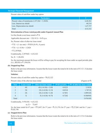
The document provides information about the Institute of Cost Accountants of India. It discusses that the Institute was established in 1959 through an Act of Parliament. It regulates the profession of cost and management accountancy. The Institute enrolls students, provides coaching and undertakes research in cost and management accounting. It pursues the vision of cost competitiveness and efficient resource use. Currently, professionals are known as 'Cost and Management Accountants' given the emphasis on management and strategic decision making. The Institute has over 500,000 students and 90,000 members globally. It operates through regional councils and chapters across India and overseas centers.


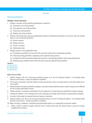
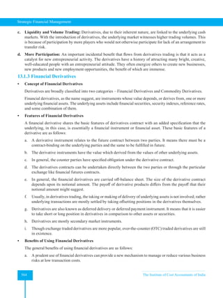
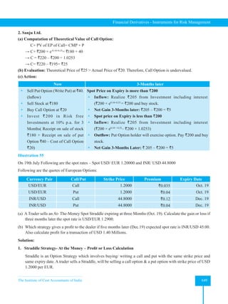
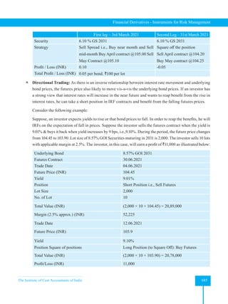
![Subject
Learning
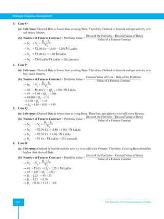
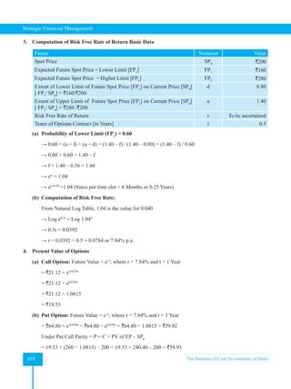
Objectives
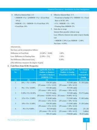
[SLOB(s)]
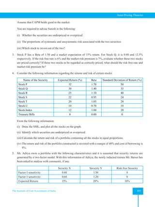
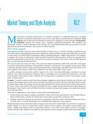
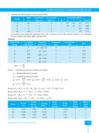
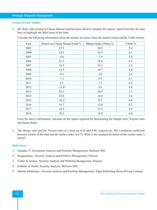
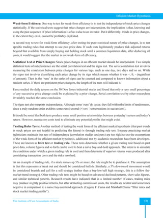
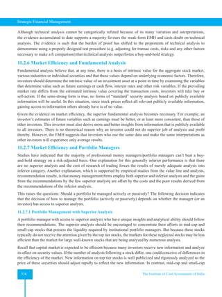
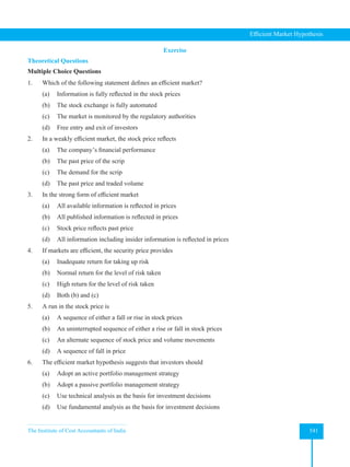
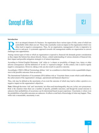
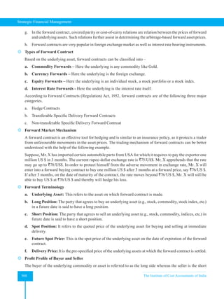
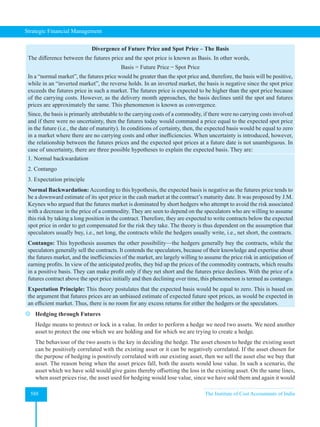
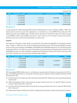
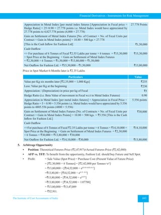
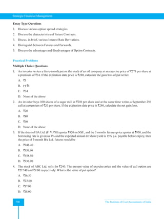
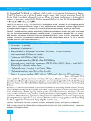
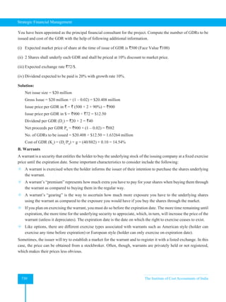
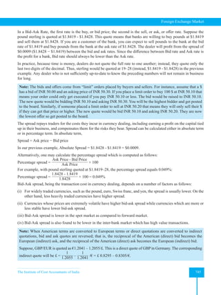
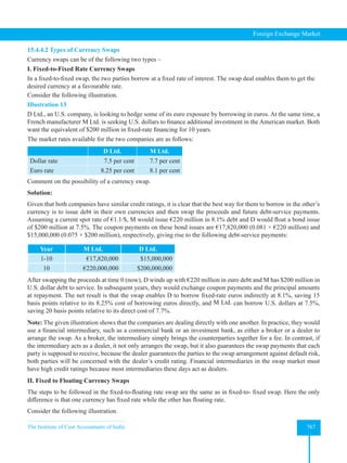
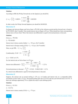
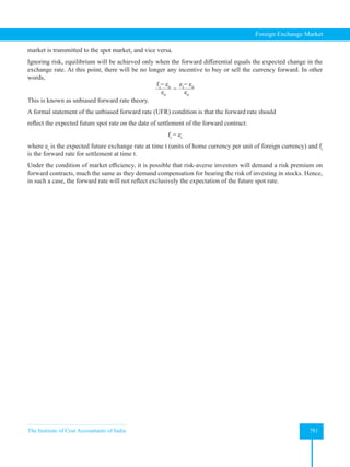
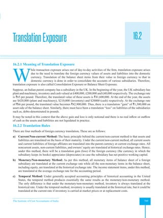
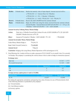
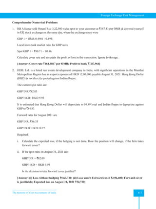
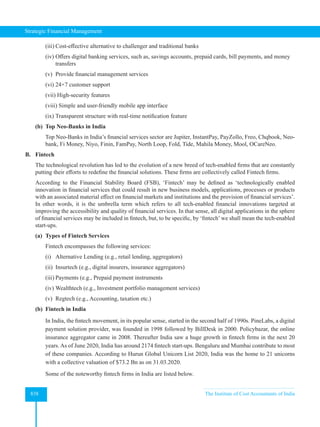
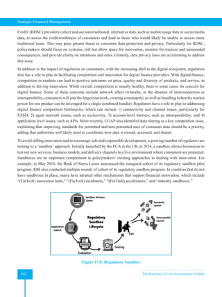
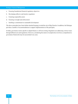
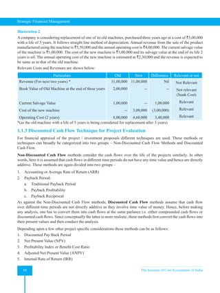
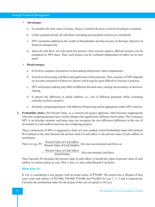
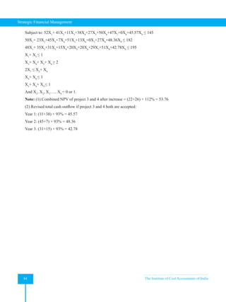
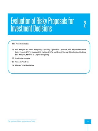
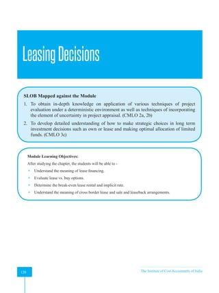
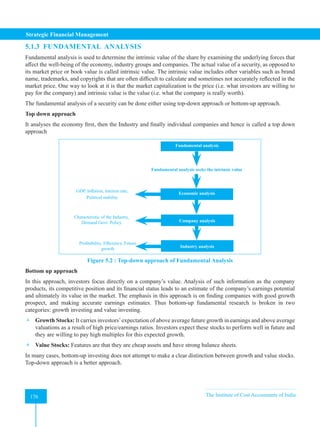
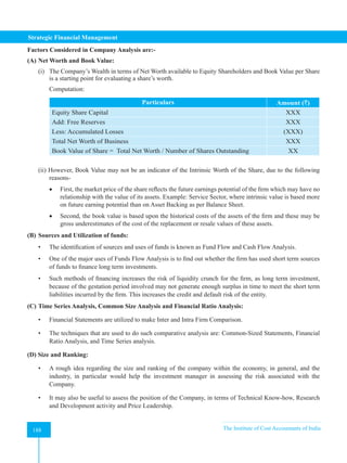
1. To obtain in-depth knowledge on application of various techniques of project evaluation under a
deterministic environment as well as techniques of incorporating the element of uncertainty in project
appraisal. (CMLO 2a, 2b)
2. To develop detailed understanding of how to make strategic choices in long term investment decisions
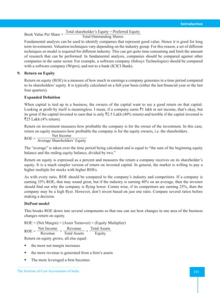
such as own or lease and making optimal allocation of limited funds. (CMLO 3c)
3. To equip oneself with the knowledge of application of various techniques in security evaluation,
building a portfolio, measuring its performance and making revisions to optimise the returns. (CMLO
3a)
4. To develop detail understanding of the sources and impact of risks to which an organisation is exposed
to in a dynamic business environment at national and international level and the techniques for
managing the same to sustain competitive advantages. (CMLO 3b, 3c)
5. To obtain an overview of various components of digital finance to better understand the interrelationship
among them. (CMLO 1a, b, c)
Subject
Learning
Outcomes
(SLOC) and
Application
Skills (APS)
SLOCs:
1. Students will be able to perform project appraisals, allocation of limited funds among competing
projects and making strategic choices in long term investment decisions.
2. They will be able to identify the risks associated with various functional areas of the organisation and
evaluate the alternative risk management techniques.
3. They will be able to build profitable portfolios and evaluate their performance continuously to identify
if any revision is warranted.
APSs:
1. They will develop necessary skill to prepare project appraisal reports and guide the management in
selecting the appropriate one.
2. They will be able to prepare risk reports to be submitted to the management to facilitate strategic
decision making relating to the functional areas of the organisation.
3. They will be able to prepare periodic portfolio performance reports to facilitate portfolio revision
decisions.
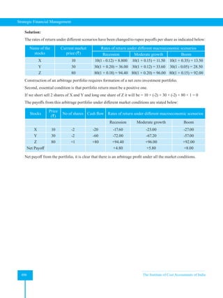
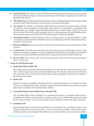
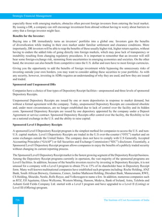
Module wise Mapping of SLOB(s)
Module
No.
Topics
Additional Resources (Research articles, books, case
studies, blogs)
SLOB Mapped
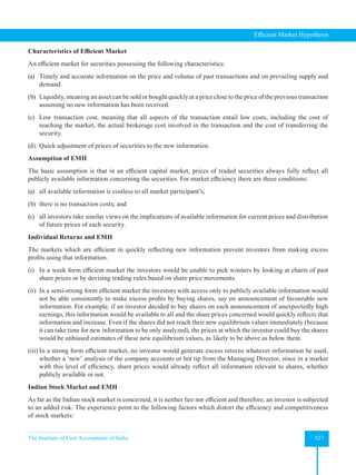
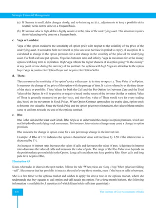
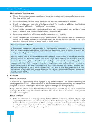
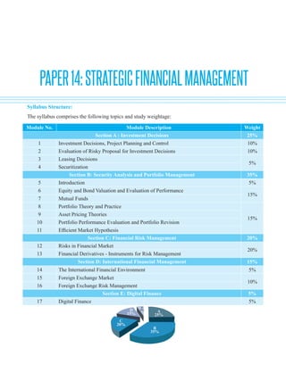
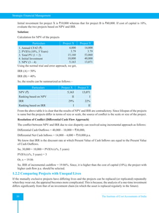
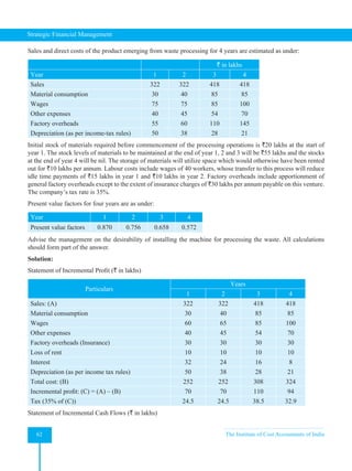
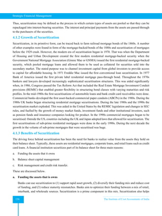
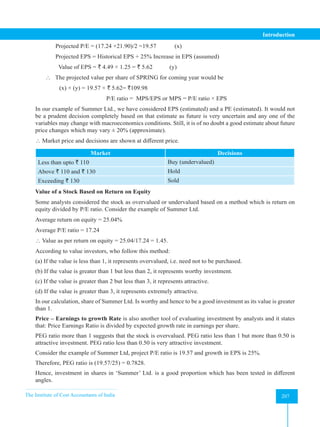
Section A: Investment Decisions
1 Investment
Decisions, Project
Planning and
Control
Capital Budgeting Techniques Among The Fortune 500: A
Rationale Approach - Burns and Walker
https://www.emerald.com/insight/content/doi/10.1108/
eb018643/full/html
1. To obtain in-depth
knowledge on
application of
various techniques
of project
evaluation under
a deterministic
environment as
well as techniques
of incorporating
the element of
uncertainty in
project appraisal.
2 Evaluation of
Risky proposal
for Investment
decisions
Capital-Budgeting Decisions Involving Combinations of
Risky Investments – J C Van Horne
https://pubsonline.informs.org/doi/abs/10.1287/
mnsc.13.2.b84
3 Leasing Decisions The Leasing Decision:AComparison of Theory and Practice
– Drury and Braund
https://www.tandfonline.com/doi/abs/10.1080/00014788
.1990.9728876](https://image.slidesharecdn.com/strategyfamous-230209132502-a14bc8e7/85/Strategy_Famous-pdf-7-320.jpg)


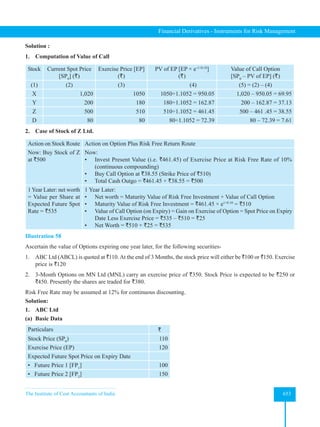
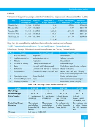
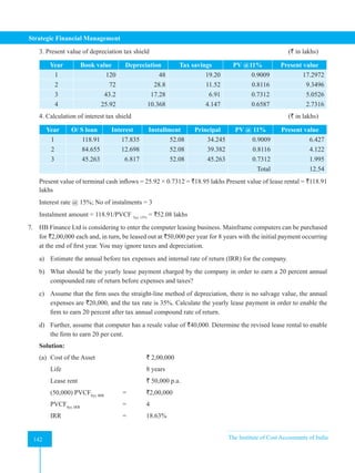
![Strategic Financial Management
8 The Institute of Cost Accountants of India
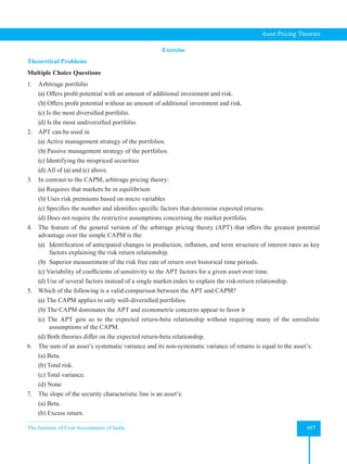
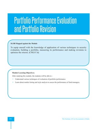
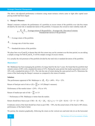
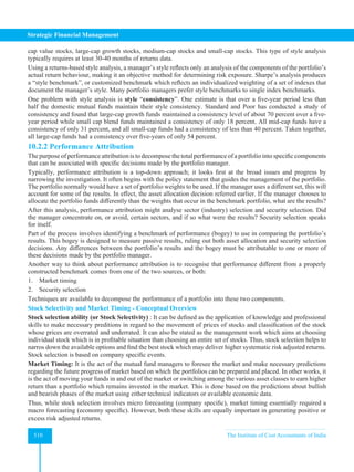
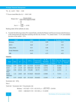
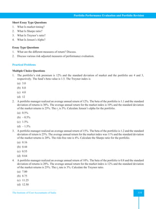
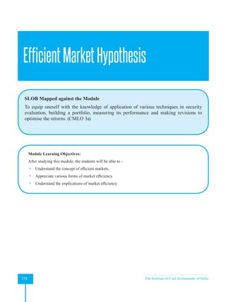
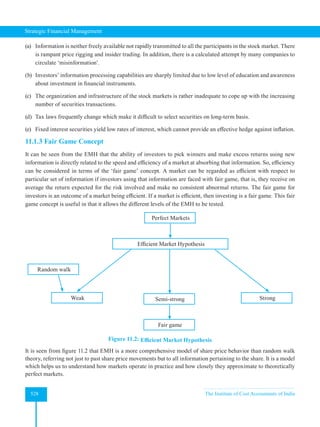
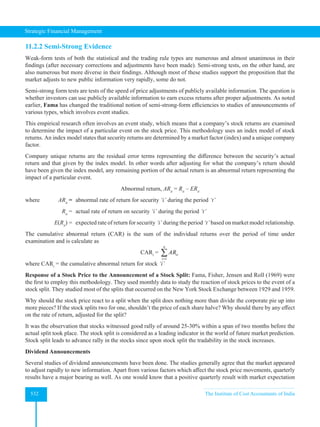
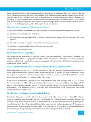
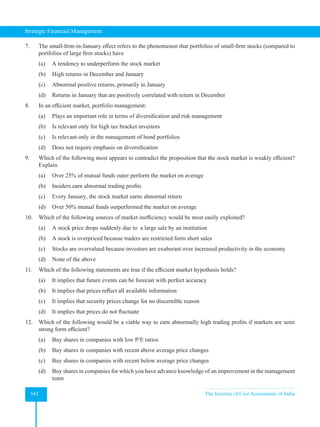
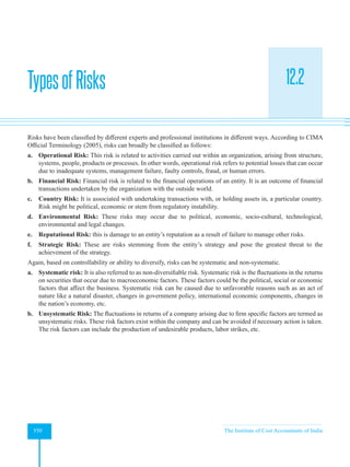
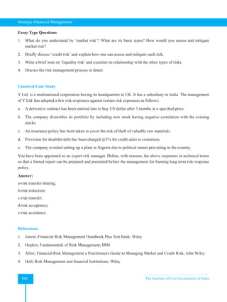
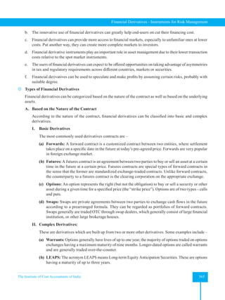
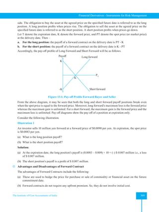
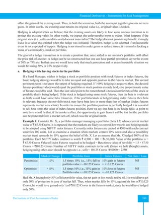
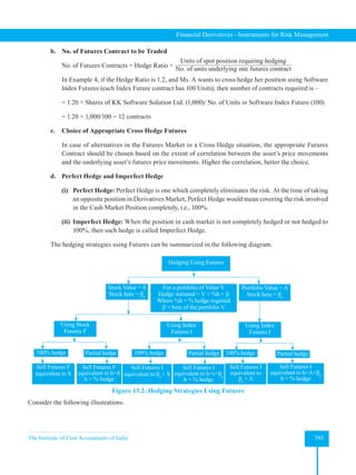
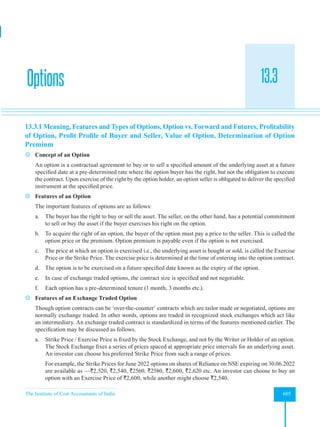
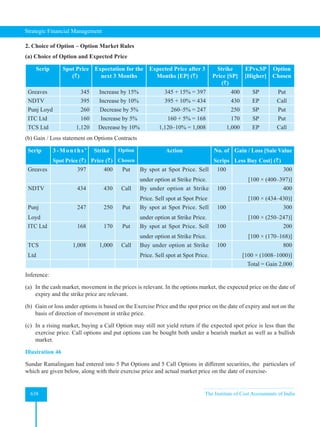
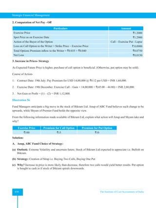
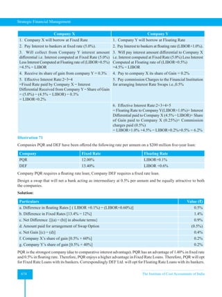
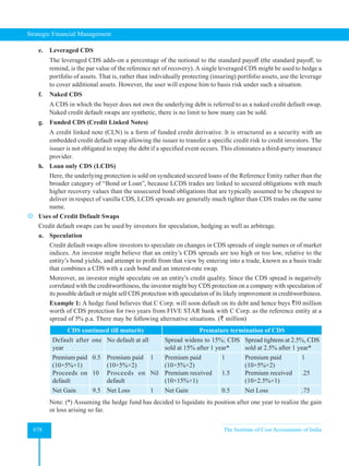
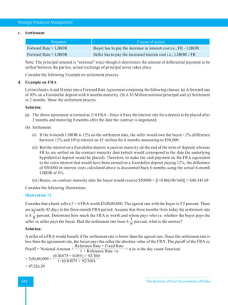
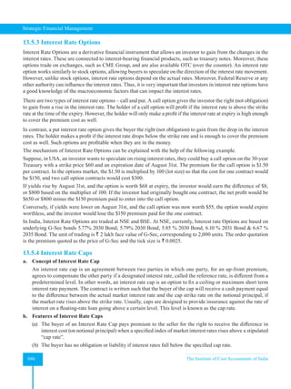
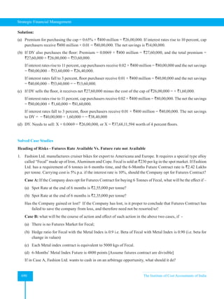
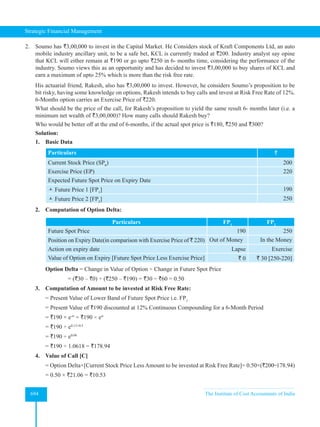
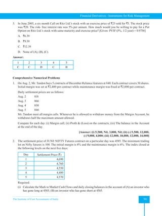
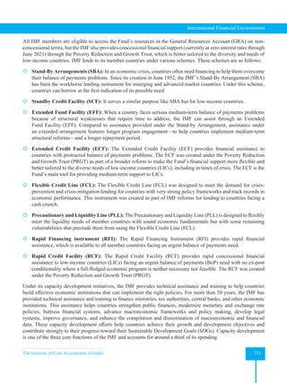
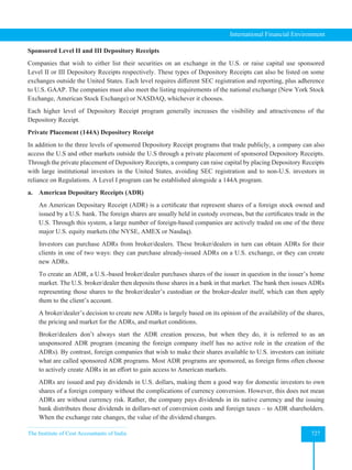
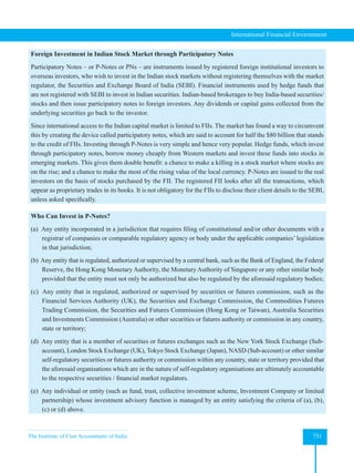
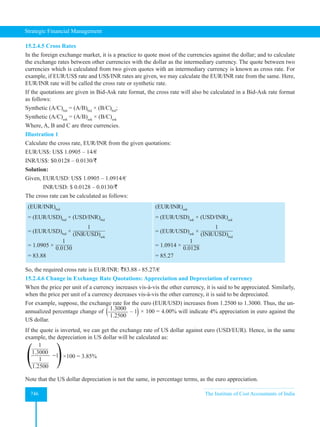
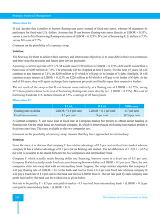
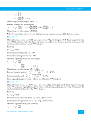
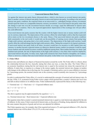
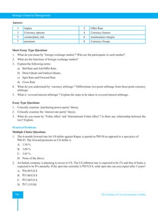
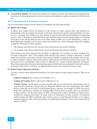
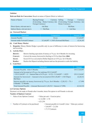
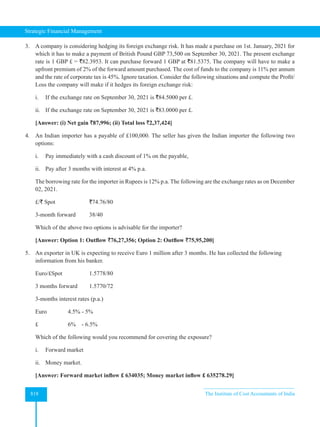
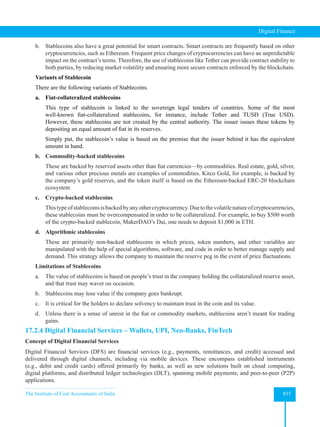
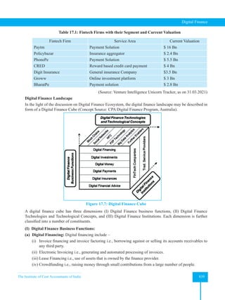
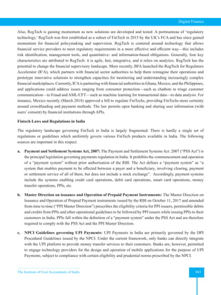
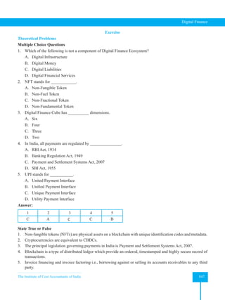
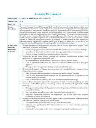
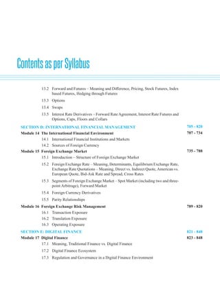
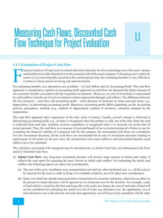
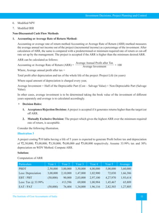
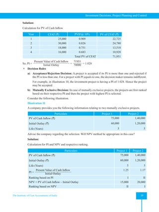
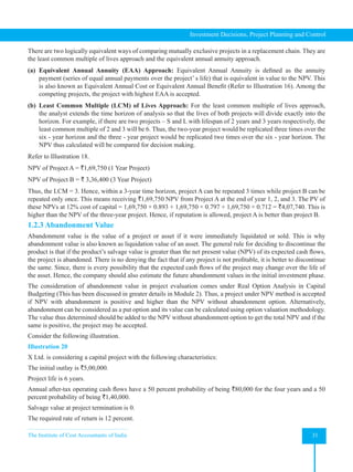
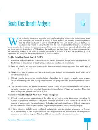
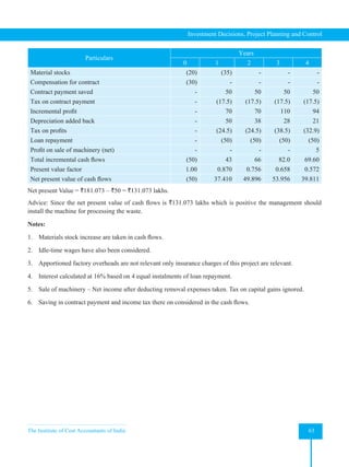
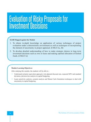
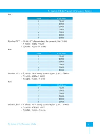
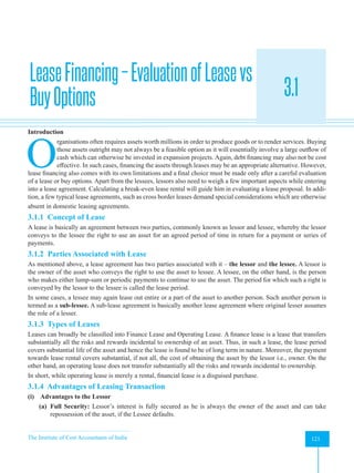
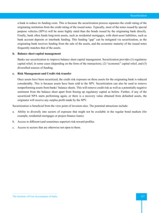
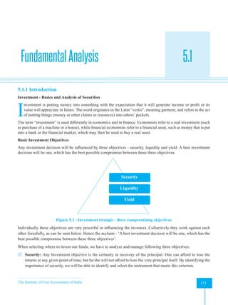
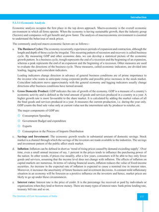
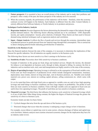
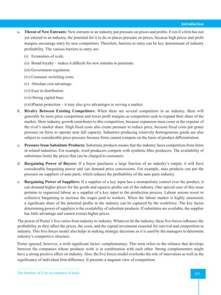
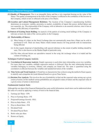
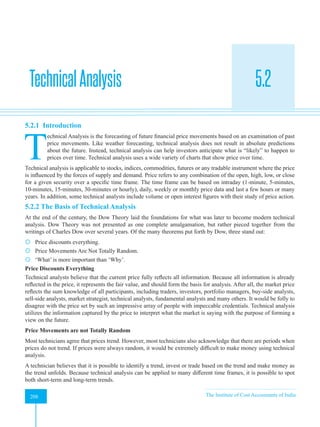
Net Cash Inflow after Taxes (CFAT):
Net Sales Revenue
Less: Cost of Goods Sold
Less: General Expenses (other than Interest)
Less: Depreciation
Profit before Interest and Taxes (PBIT or EBIT)
Less: Taxes
Profit after Taxes (excluding Interest) [PAT]
Add: Depreciation
Net Cash Inflow after Taxes
In short, CFAT = EBIT (1 – t) + Depreciation [where, t is income tax rate]
Note: If PAT is taken from accounting records, which is arrived at after charging Interest, ‘Interest Net
of Taxes’ is to be added back along with the amount of Depreciation, i.e.,
PAT after charging Interest
Add: Depreciation
Add: Interest Net of Taxes (i.e., Total Interest – Tax on Interest)
Net Cash Inflow after Taxes
Consider the following illustration.
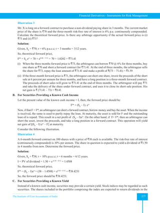
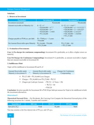
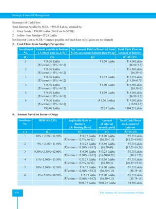
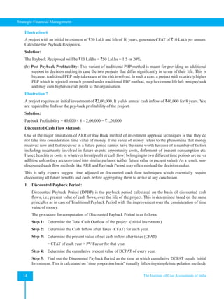
Illustration 1
` `
Net Sales Revenue 10,00,000
Less: Cost of Goods Sold 5,00,000
Less: Operating Expenses 2,00,000
Less: Depreciation 1,00,000 8,00,000
PBIT or EBIT 2,00,000
Less: Interest 50,000
PBT or EBT 1,50,000
Less: Tax (30%) 45,000
PAT 1,05,000
Net Cash Inflow after Taxes: `
EBIT 2,00,000
Less: Tax (30%) 60,000
1,40,000
Add: Depreciation 1,00,000
Net Cash Inflow after Taxes 2,40,000](https://image.slidesharecdn.com/strategyfamous-230209132502-a14bc8e7/85/Strategy_Famous-pdf-20-320.jpg)
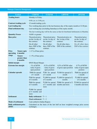
![The Institute of Cost Accountants of India 35
Investment Decisions, Project Planning and Control
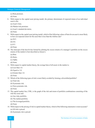
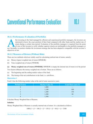
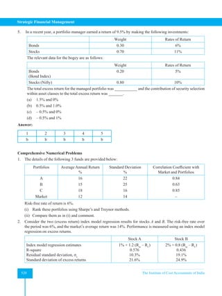
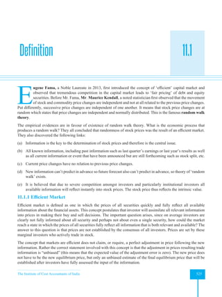
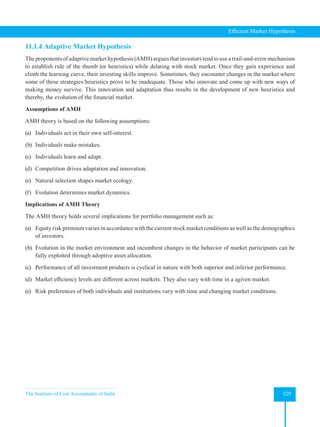
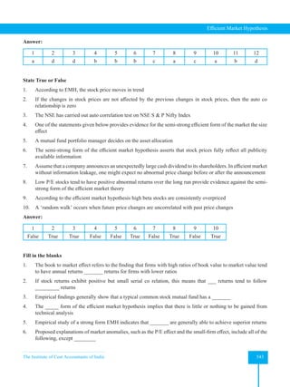
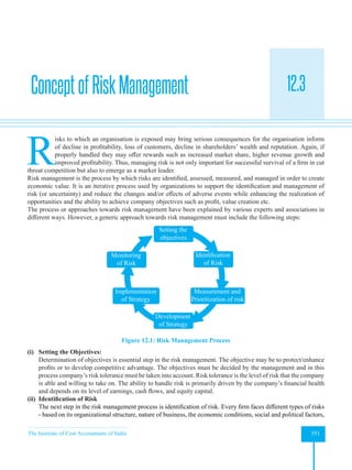
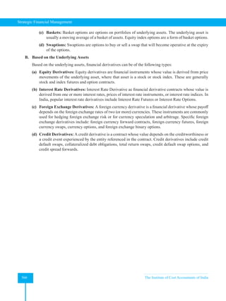
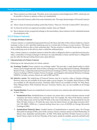
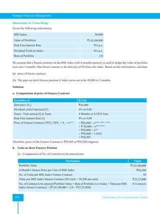
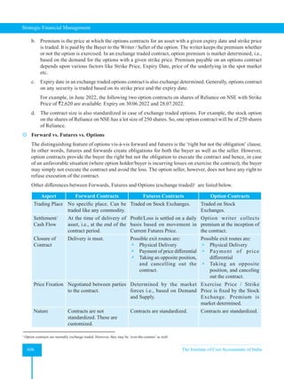
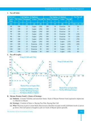
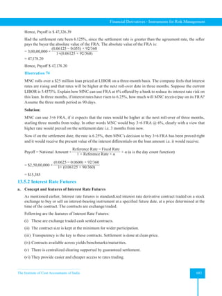
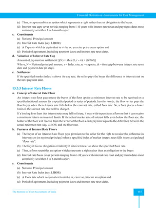
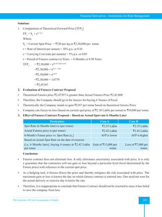
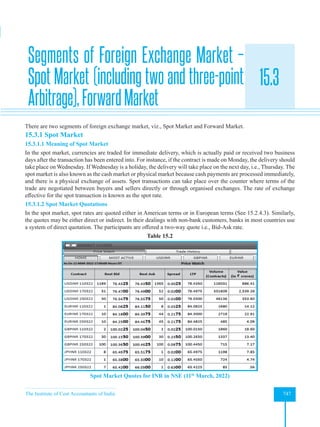
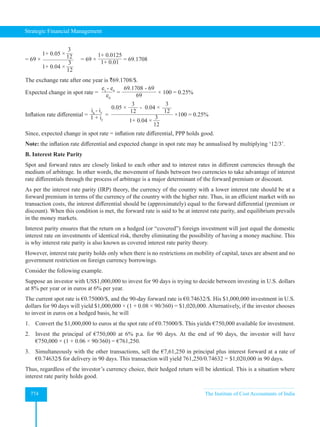
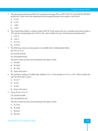
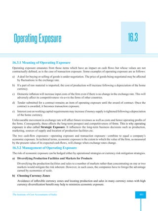
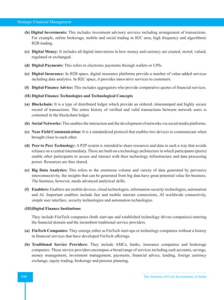
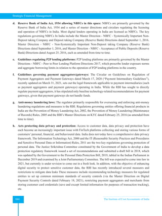
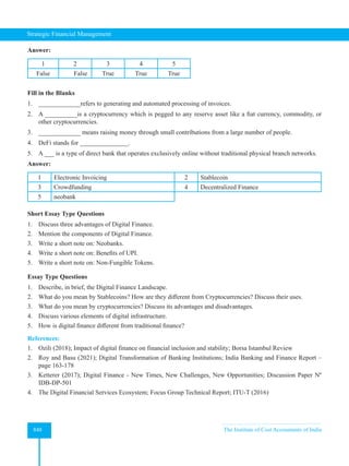
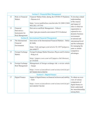
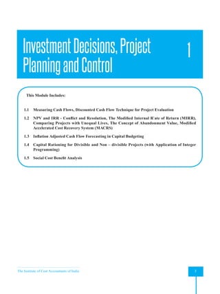
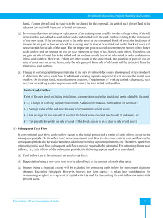
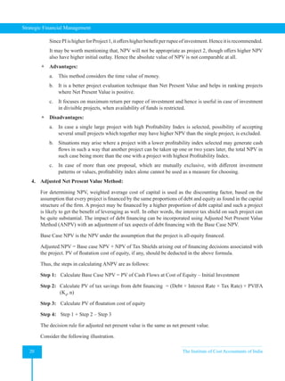
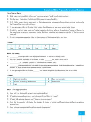
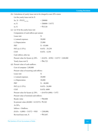
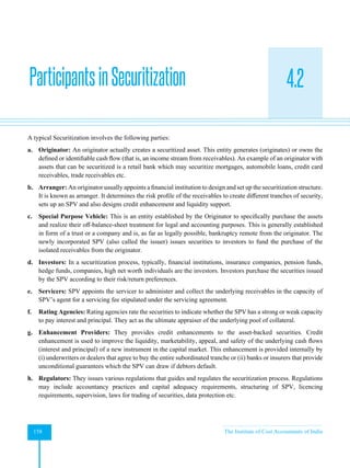
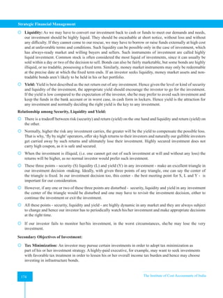
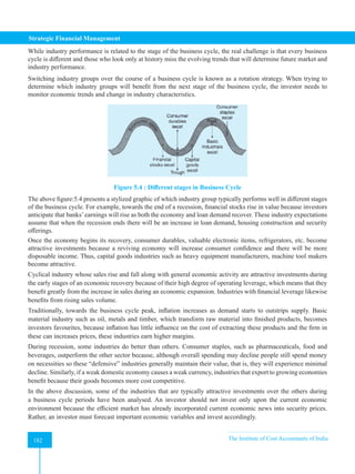
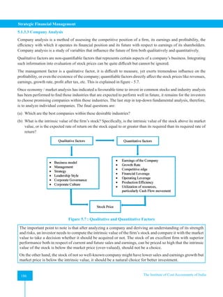
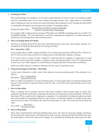
Alternatively,
Present Value of Real Cash Flows = Nominal Cash Flows of the period ‘t’ ÷ (1+ NDR)t
It may be noted that Nominal or Money Cash Flows are the actual amount expected to arise in future while Real
Cash Flows are the nominal cash flows expressed in terms of real values representing purchasing power. Therefore,
it is prudent to use the real cash flows for analysis instead of money or nominal cash flows.
1.3.3 Relationship between NDR and RDR
The relationship between NDR and RDR can be expressed in form of the following equation:
1 + Nominal Discount Rate = (1 + Real Discount Rate) (1 + Inflation Rate)
or, NDR = (1 + RDR) (1 + IR) – 1
It may be observed from the above equation that Nominal Discount Rate contains two elements – Real Discount
Rate and Inflation Rate. Real Discount Rate helps maintaining the shareholders wealth and Inflation Rate is the
compensation for giving up the purchasing power today for a purchasing power in future.
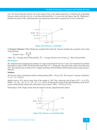
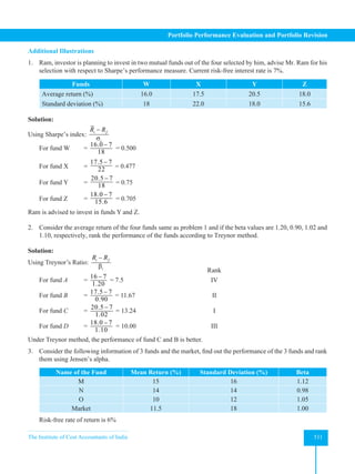
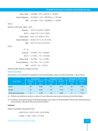
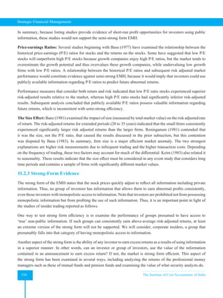
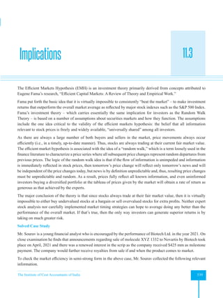
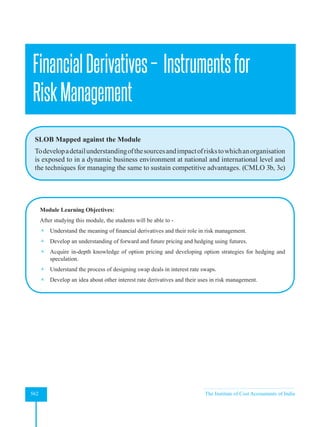
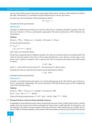
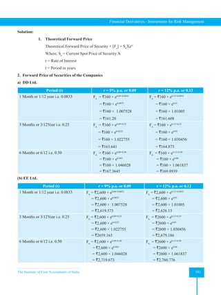
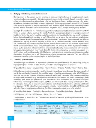
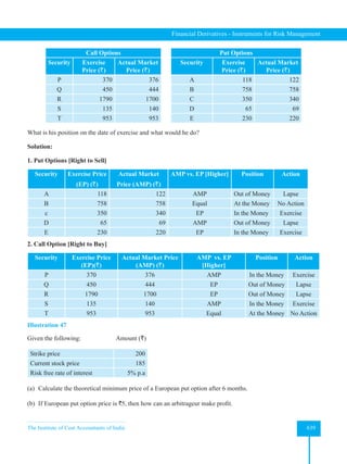
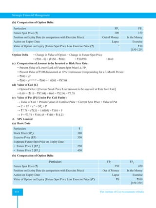
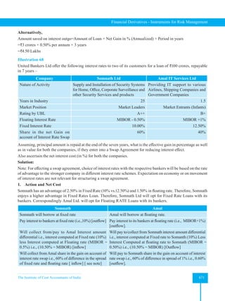
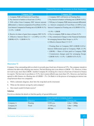
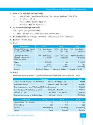
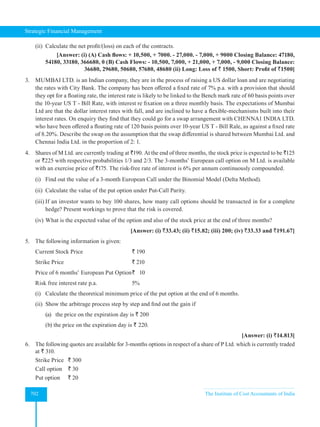
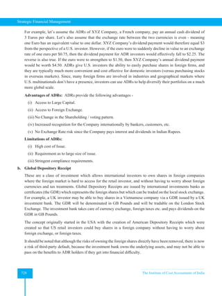
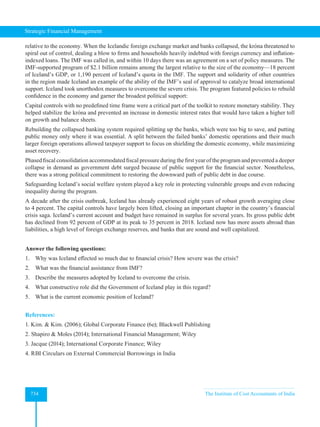
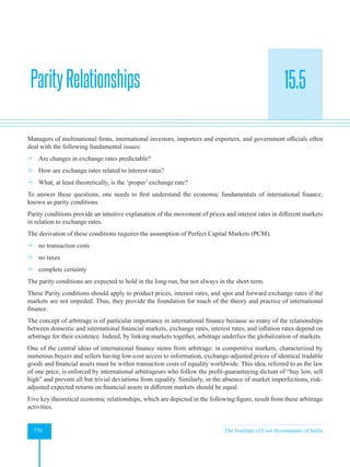
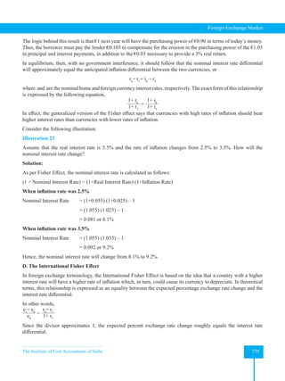
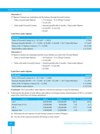
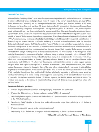
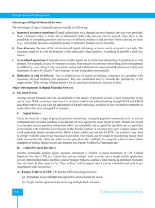
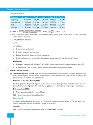
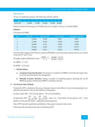
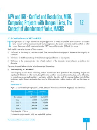
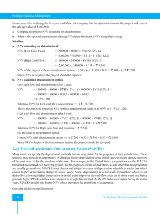
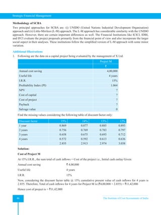
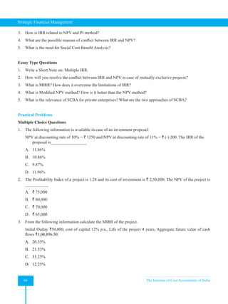
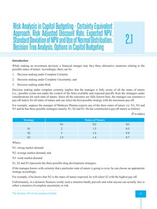
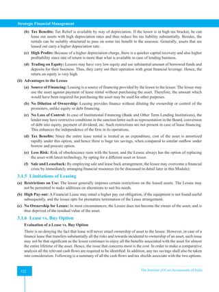
Illustration 22
The following information is available:
Initial Outlay `24 lakh. Life 4 years. Annual PBDT `10 lakh. Income Tax Rate 40%. Inflation Rate 5%. Real
Discount Rate (Cost of Capital 10%).
In absence of Inflation:
Year PBDT Depreciation PBT Tax PAT Cash Flow
0 – 24,00,000
1 – 4 10,00,000 6,00,000 4,00,000 1,60,000 2,40,000 8,40,000
Calculate NPV before and after adjustment of inflation and comment on the viability of the project.
Solution:
In absence of Inflation, NPV will be as follows:
PV of Cash Inflows = 8,40,000 × (0.9091 + 0.8264 + 0. 7513 + 0.6830) = `26,62,632
Less: PV of Cash Outflows (Initial Outlay) = `24,00,000
NPV =
` 2,62,632
As the NPV is positive, the project is acceptable.
With 5% Inflation, Nominal Cash Inflow will be discounted with Inflation Rate for finding out the Real Cash Flow
and thereafter Real Cash Inflow will be discounted with Real Discount Rate to get the present value.
Year 1 2 3 4
Nominal Cash Inflow after Tax (`): 8,40,000 8,40,000 8,40,000 8,40,000
Real Cash Inflow 8,00,000 7,61,905 7,25,624 6,91,070
[(Nominal Cash Inflow / (1+ Inflation Rate)]
PV of Real Cash Inflow 7,27,273 6,29,674 5,45,172 4,72,010
[(Real Cash Flow / (1+ Real Discount Rate, K)]](https://image.slidesharecdn.com/strategyfamous-230209132502-a14bc8e7/85/Strategy_Famous-pdf-47-320.jpg)
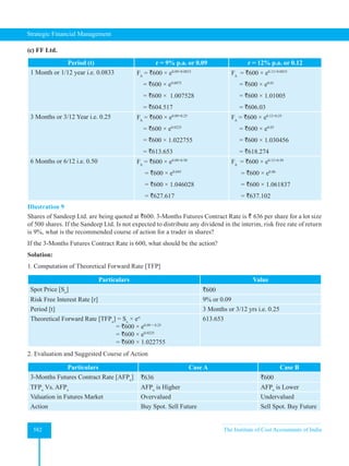
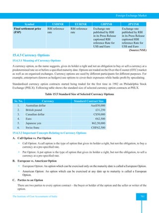
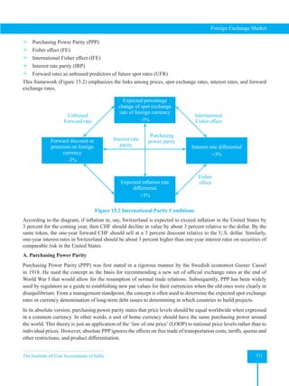
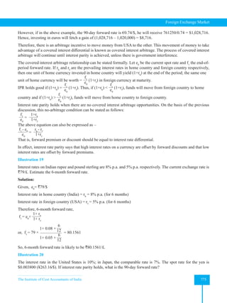
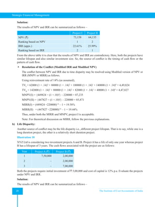
![Strategic Financial Management
36 The Institute of Cost Accountants of India
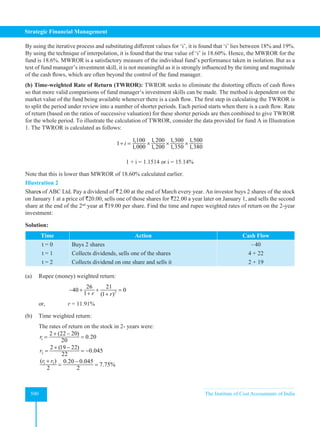
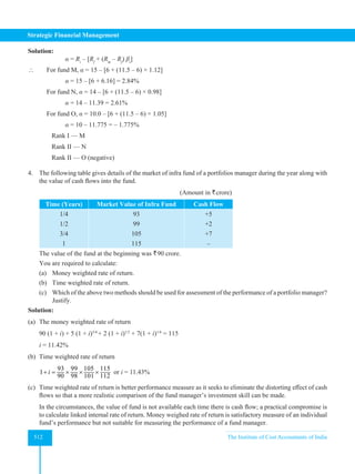
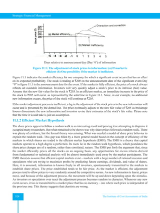
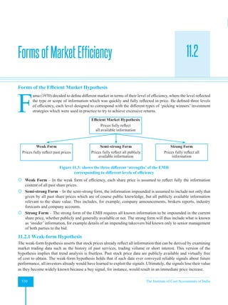
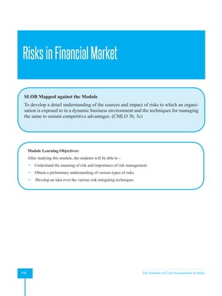
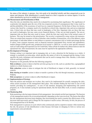
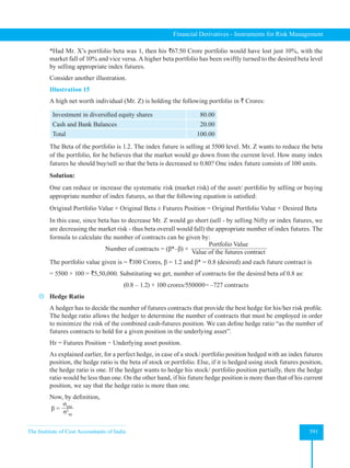
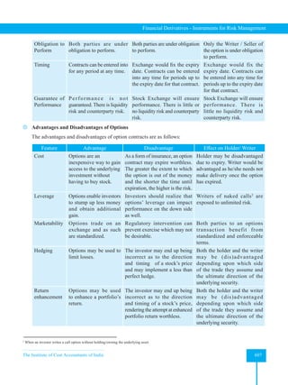
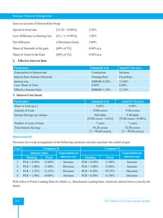
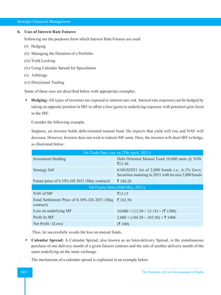
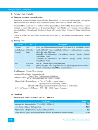
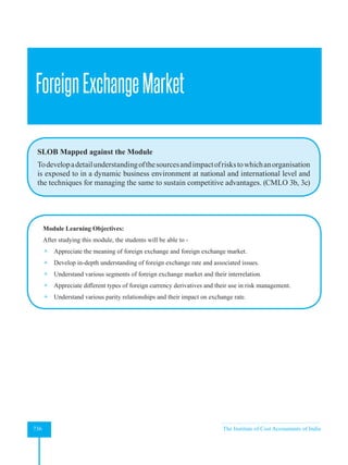
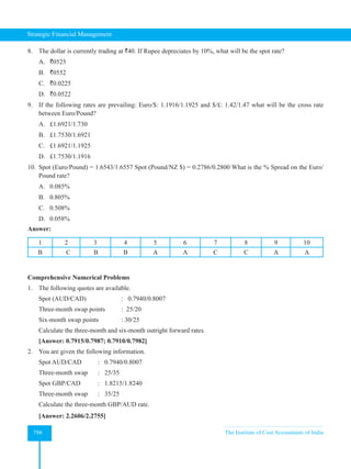
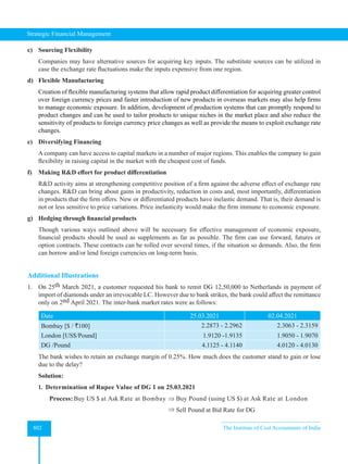
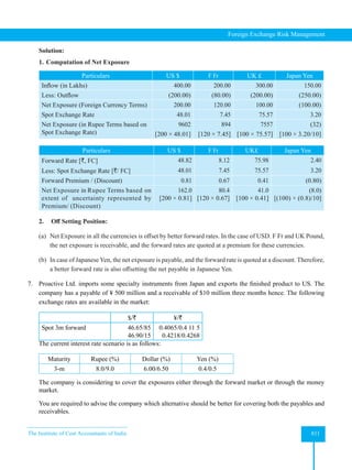
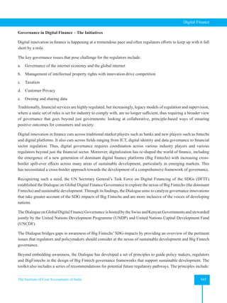
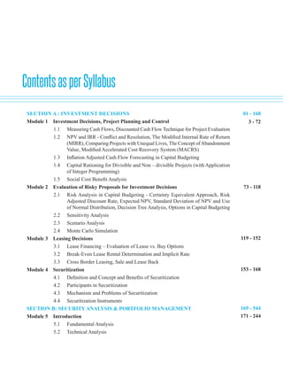
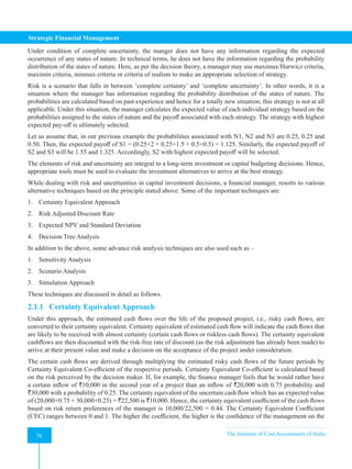
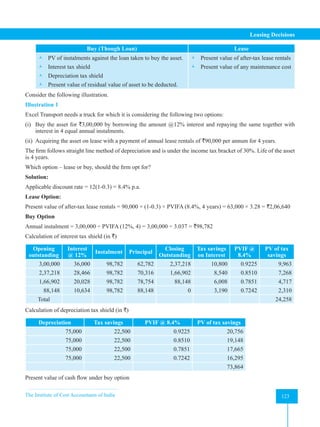
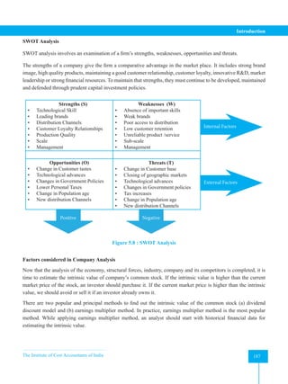
Total PV of Real Cash Inflows: ` 23,74,129
PV of Cash Outflow (Initial Outlay): ` 24,00,000
NPV ` (–) 25,871
The project is not acceptable as NPV is negative.
Alternatively, the Nominal Cash Inflows may be discounted with the Nominal Discount Rate.
Nominal Discount Rate = 1 – (1+IR) (1+RDR)
NDR = 1 – (1+0.05) (1+0.10) = 1 – 1.155 = 0.155 or 15.5%
PV of Real Cash Inflows = 8,40,000 × [(
1
1.155
)1
+ (
1
1.155
)2
+ (
1
1.155
)3
+ (
1
1.155
)4
] = ` 23,74,176
NPV (after considering inflation) = ` (23,74,176 – 24,00,000) = ` (–) 25,824
[Note: Two results are same, difference between two figures (`25,871 & `25,824) is due to approximation of
discounting factors.]
The project is not acceptable as NPV is negative.](https://image.slidesharecdn.com/strategyfamous-230209132502-a14bc8e7/85/Strategy_Famous-pdf-48-320.jpg)
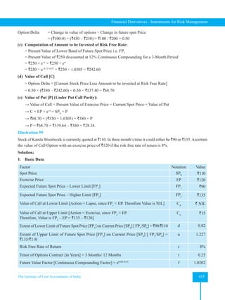
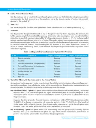
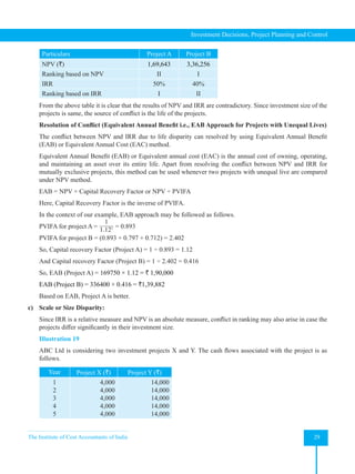
![Strategic Financial Management
48 The Institute of Cost Accountants of India
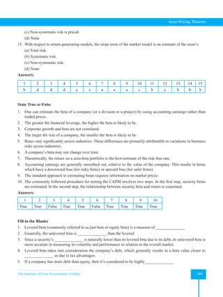
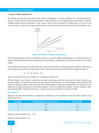
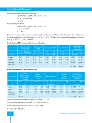
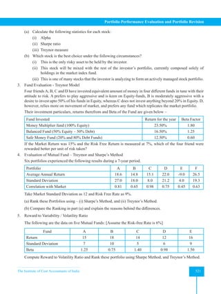
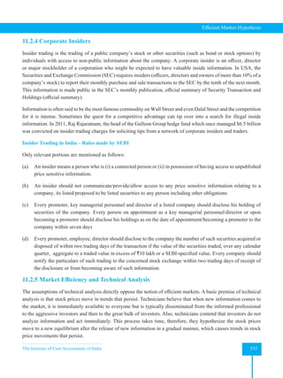
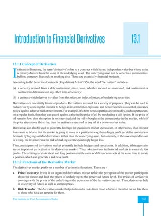
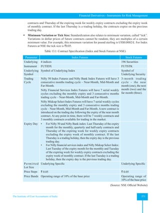
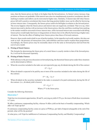
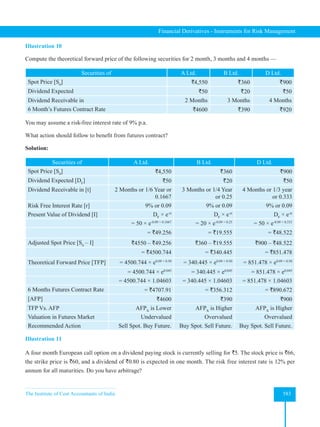
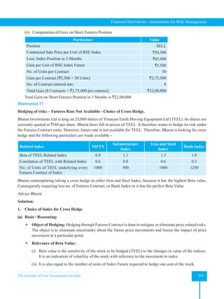
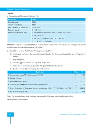
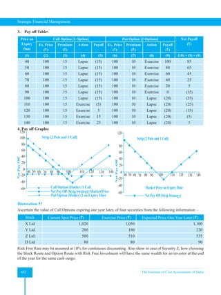
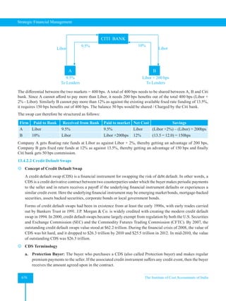
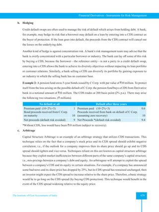
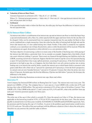
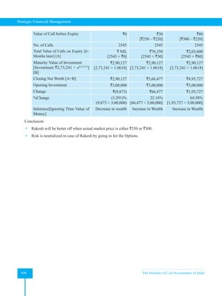
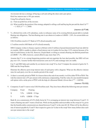
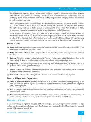
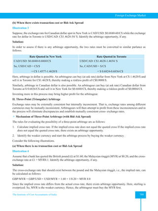
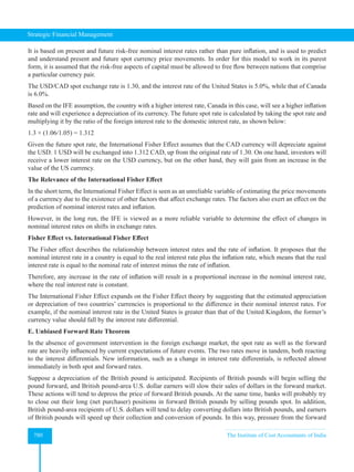
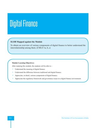
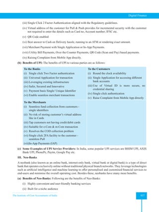
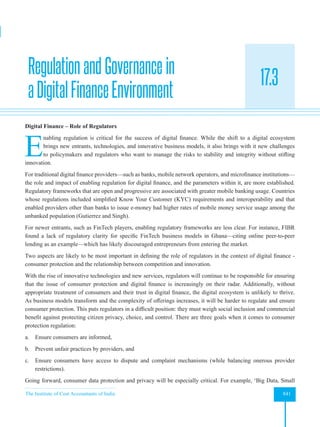
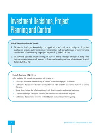
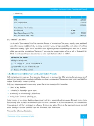
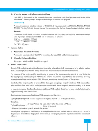
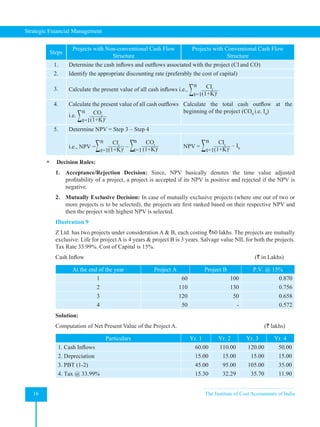
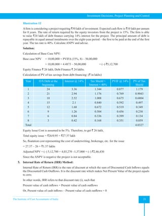
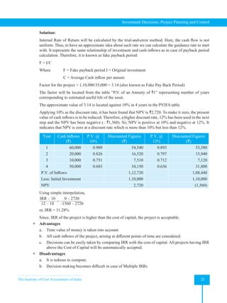
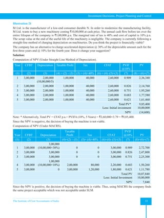
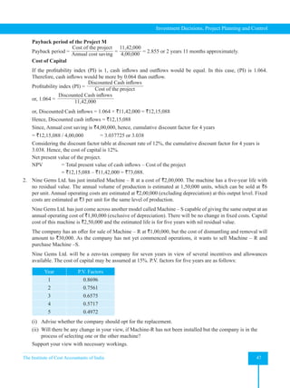
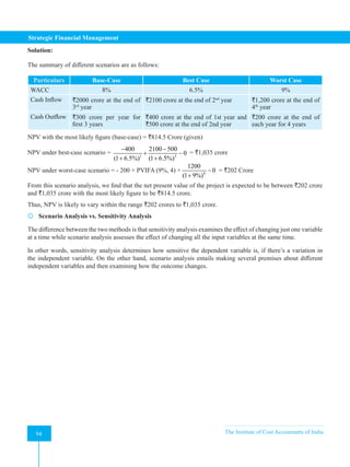
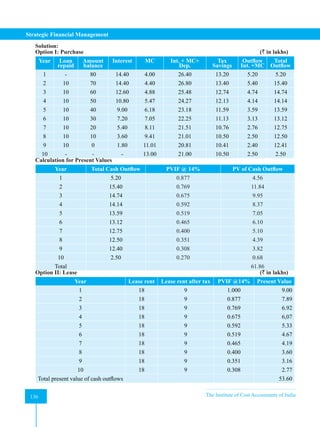
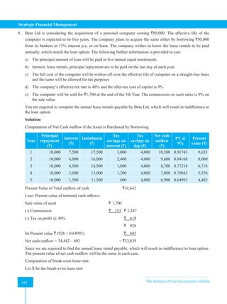
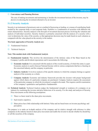
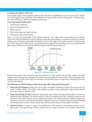
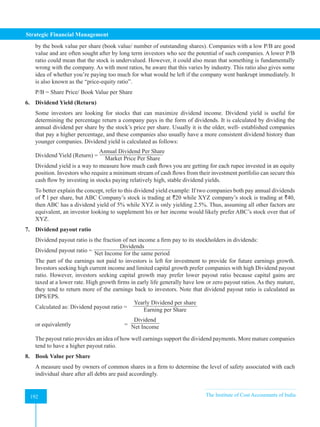
Solution:
(i) Replacement of Machine – R:
Incremental cash out flow
Particulars ` `
(i) Cash outflow on Machine – S 2,50,000
Less: Sale value of Machine – R
Less: Cost of dismantling and removal
1,00,000
30,000 70,000
Net outflow 1,80,000
Incremental cash flow from Machine –S
Annual cash flow from Machine – S [(1,50,000×`6)–(1,50,000× `3) –
1,80,000]
2,70,000
Annual cash flow from Machine – R [(1,50,000×`6)– (1,50,000×`3) –
2,00,000]
2,50,000
Net incremental cash in flow 20,000
Present value of incremental cash inflows = `20,000 × (0.8696 + 0.7561 + 0.6575 + 0.5717 + 0.4972)
= `20,000 × 3.3523 = `67,046
NPV of Machine – S = `67,046 – `1,80,000 = (–) `1,12,954.
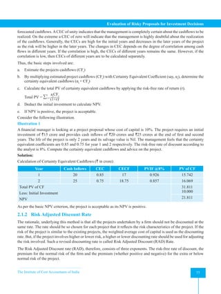
`2,00,000 spent on Machine – R is a sunk cost and hence it is not relevant for deciding the replacement.
Decision: Since Net present value of Machine –S is in the negative, replacement is not advised.
If the company is in the process of selecting one of the two machines, the decision is to be made on the
basis of independent evaluation of two machines by comparing their Net present values.
(ii) Independent evaluation of Machine– R and Machine –S
Particulars Machine– R Machine– S
Units produced 1,50,000 1,50,000
Selling price per unit (`) 6 6
Sale value 9,00,000 9,00,000
Less: Operating Cost (exclusive of depreciation) 2,00,000 1,80,000
Contribution 7,00,000 7,20,000
Less: Fixed cost 4,50,000 4,50,000
Annual Cash flow 2,50,000 2,70,000
Present value of cash flows for 5 years 8,38,075 9,05,121
Cash outflow 2,00,000 2,50,000
Net Present Value 6,38,075 6,55,121
As the NPV of Cash in flow of Machine-S is higher than that of Machine-R, the choice should fall on
Machine-S.
Note: As the company is a zero tax company for seven years (Machine life in both cases is only for five
years), depreciation and the tax effect on the same are not relevant for consideration.](https://image.slidesharecdn.com/strategyfamous-230209132502-a14bc8e7/85/Strategy_Famous-pdf-60-320.jpg)
![Strategic Financial Management
54 The Institute of Cost Accountants of India
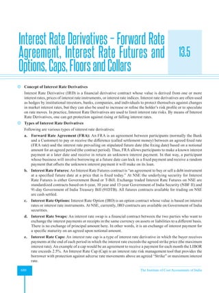
Computation of Equity IRR
Equity IRR is computed by using the following equation:
Cash inflow at zero date from equity shareholders = ∑Cash inflow available for equity shareholders
(1+r)n
Where,
r = Equity IRR
n = Life of the project
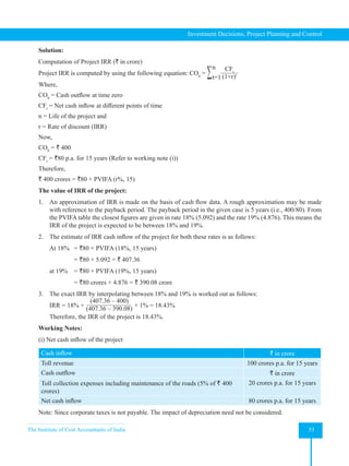
Here, Cash inflow at zero date from equity shareholders = `100 crores
Cash inflow for equity shareholders = `28.69 crores p.a. (Refer to working note).
Therefore: `100 crores = ∑`28.69
(1+r)n
The value of equity IRR of the project is calculated as follows:
An approximation of IRR is made on the basis of cash flow data. A rough approximation may be made with
reference to the payable period. The payback period in the given case is 3.484 (100/28.69)
From the PVIFA table at 28% the cumulative discount factor for 1 –15 years is 3.484. Therefore, the equity
IRR of project is 28%.
(ii) Equated annual instalment (i.e., principal + interest) of loan from financial institution:
Amount of loan from financial institution (` in crore) ` 300
Rate of interest 15% p.a.
No. of years 15
Cumulative discount factor for 1-15 years 5.847
Hence, equated yearly instalment will be `300 crores/5.847 i.e., `51.31crore.
(iii) Cash inflow available for equity shareholders
Net cash inflow of the project [Refer to working note (i)] ` 80.00
Equated yearly instalment of the project [Refer to working note (ii)] ` 51.31
Cash inflow available for equity shareholders ` 28.69
Difference in Project IRR and Equity IRR:
The project IRR is 18.4% whereas Equity IRR is 28%. This is attributed to the fact that XYZ Ltd. is earning
18.4% on the loan from financial institution but paying only 15%. The difference between the return and cost
of funds from financial institution has enhanced equity IRR. The 3.4% (18.4% - 15%) earnings on `300 crores
goes to equity shareholders who have invested `100 crore i.e.,
3.4% × `300/`100 = 10.2% is added to the project IRR is equity IRR of 28%.
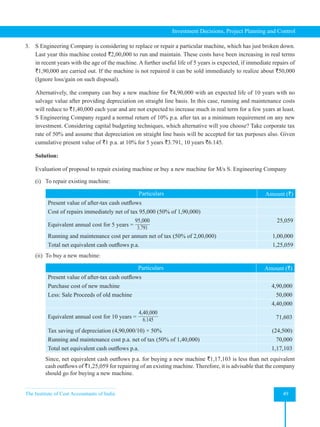
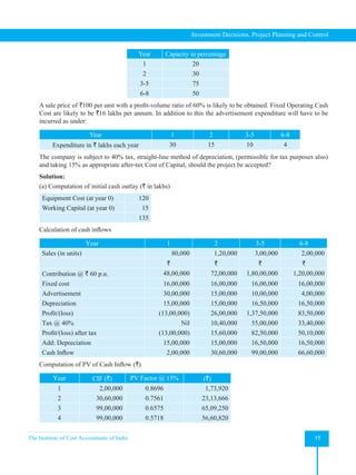
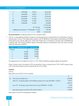
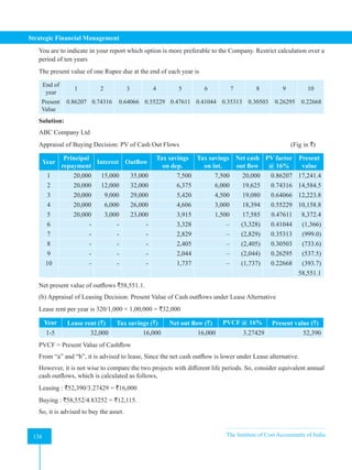
6. X Ltd. an existing profit-making company, is planning to introduce a new product with a projected life of 8
years. Initial equipment cost will be `120 lakhs and additional equipment costing `10 lakhs will be needed at
the beginning of third year. At the end of the 8 years, the original equipment will have resale value equivalent
to the cost of removal, but the additional equipment would be sold for `1 lakhs. Working Capital of `15 lakhs
will be needed. The 100% capacity of the plant is of 4,00,000 units per annum, but the production and sales-
volume expected are as under:](https://image.slidesharecdn.com/strategyfamous-230209132502-a14bc8e7/85/Strategy_Famous-pdf-66-320.jpg)
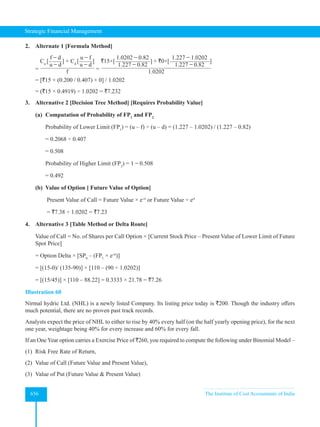
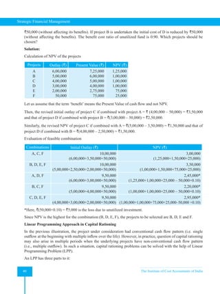
![Strategic Financial Management
58 The Institute of Cost Accountants of India
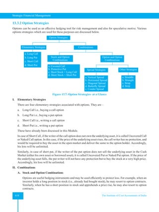
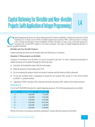
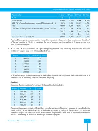
Statement showing NPV of the projects
Project Amount (`) P.I. Cash inflows of project (`) N.P.V. of Project (`)
(i) (ii) (iii) (iv) = [(ii) × (iii)] (v) = [(iv) – (ii)]
1 3,00,000 1.22 3,66,000 66,000
2 1,50,000 0.95 1,42,500 (-)7,500
3 3,50,000 1.20 4,20,000 70,000
4 4,50,000 1.18 5,31,000 81,000
5 2,00,000 1.20 2,40,000 40,000
6 4,00,000 1.05 4,20,000 20,000
The allocation of funds to the projects 1, 3 and 5 (as selected above on the basis of P.I.) will give N.P.V. of
`1,76,000 and `1,50,000 will remain unspent.
However, the N.P.V. of the projects 3, 4 and 5 is `1,91,000 which is more than the N.P.V. of projects 1, 3 and
5. Further, by undertaking projects 3, 4 and 5 no money will remain unspent. Therefore, S Ltd. is advised to
undertake investments in projects 3, 4 and 5.
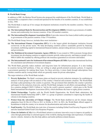
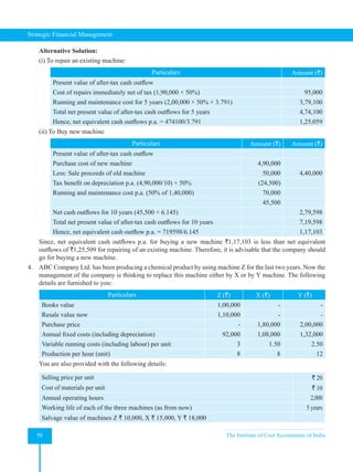
9. A product is currently manufactured on a machine that is not fully depreciated for tax purposes and has a book
value of `70,000. It was purchased for `2,10,000 twenty years ago. The cost of the product are as follows:
Particulars Unit Cost (`)
Direct Labour 28.00
Indirect labour 14.00
Other variable overhead 10.50
Fixed overhead 17.50
70.00
In the past year 10,000 units were produced. It is expected that with suitable repairs the old machine can be
used indefinitely in future. The repairs are expected to average `75,000 per year.
An equipment manufacturer has offered to accept the old machine as a trade in for a new equipment. The
new machine would cost `4,20,000 before allowing for `1,05,000 for the old equipment. The Project costs
associated with the new machine are as follows:
Particulars Unit Cost (`)
Direct Labour 14.00
Indirect labour 21.00
Other variable overhead 7.00
Fixed overhead 22.75
64.75
The fixed overhead costs are allocations for other departments plus the depreciation of the equipment. The old
machine can be sold now for `50,000 in the open market. The new machine has an expected life of 10 years
and salvage value of `20,000 at that time. The current corporate income tax rate is assumed to be 50%. For tax
purposes cost of the new machine and the book value of the old machine may be depreciated in 10 years. The
minimum required rate is 10%. It is expected that the future demand of the product will stay at 10,000 units per
year. The present value of an annuity of `1 for 9 years @ 10% discount factor = 5.759. The present value of `1](https://image.slidesharecdn.com/strategyfamous-230209132502-a14bc8e7/85/Strategy_Famous-pdf-70-320.jpg)
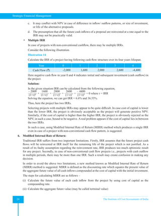
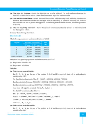
![The Institute of Cost Accountants of India 59
Investment Decisions, Project Planning and Control
received at the end of 10th year @ 10% discount factor is = 0.386. Should the new equipment be purchased?
Solution:
Evaluation of replacement decision under NPV Method
Step 1: Calculation of PV of net cash outflow
Cost of new machine 4,20,000
Less: Exchange price for old machine 1,05,000
3,15,000
Add: Tax on profit on exchange [1,05,000 – 70,000 = 35,000×50%]= 17,500
Net Investment = 3,32,500
Step 2: Calculation of PV of incremental operating cash inflows for 10 years
Existing New Incremental
Number of units 10,000 10,000 –
` ` `
Variable cost per unit 52.5 42 10.5
Variable Cost 5,25,000 4,20,000 1,05,000
Repairs 75,000 -- 75,000
Depreciation 7,000 40,000 [33,000]
[2,10,000 – 70,000]/20
[4,20,000 – 20,000]/10
Total Savings before tax 1,47,000
Less: Tax at 50% 73,500
Savings after tax 73,500
Add: Depreciation 33,000
CFAT 1,06,500
Note: The allocations from other department are irrelevant for decision making.
Step 3: Calculation of terminal cash inflows
Salvage value of machine = `20,000
Step 4: Calculation of NPV:
Operating cash inflow from 1 to 9 years [1,06,500 × 5.759] = 6,13,334
PV of cash inflow for 10th year (1,06,500 + 20,000) × 0.386 = 48,829
PV of total cash inflow = 6,62,163
Less: Outflow = 3,32,500
NPV = 3,29,663
Comment: Since NPV is positive, it is advised to replace the machine.
Note: Since the exchange value is greater than open market value, the open market value is irrelevant.
Working Notes:
1. Calculation of Operating Cash Inflows](https://image.slidesharecdn.com/strategyfamous-230209132502-a14bc8e7/85/Strategy_Famous-pdf-71-320.jpg)
![Strategic Financial Management
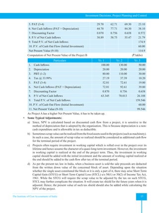
60 The Institute of Cost Accountants of India
Year Production Contribution Fixed
expenses
Depreciation
(WDV)
PBT PAT CIAT PV at 15% PV
1
2
3
4
5
6
400
800
1080
1200
1200
1200
320
640
864
960
960
960
240
360
480
480
480
480
200
133
89
59
40
26
(120)
147
295
421
440
454
(60)
74
148
210
220
227
140
207
237
269
260
253
0.870
0.756
0.658
0.572
0.497
0.432
121.80
156.49
155.95
153.87
129.22
109.29
PV of operating cash inflows for 6 years 826.62
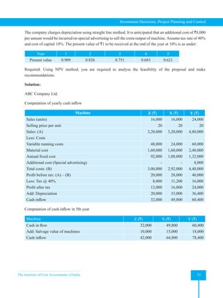
10. Techtronics Ltd., an existing company, is considering a new project for manufacture of pocket video games
involving a capital expenditure of `600 lakhs and working capital of `150 lakhs. The capacity of the plant is
for an annual production of 12 lakh units and capacity utilisation during the 6-year working life of the project
is expected to be as indicated below.
Year Capacity utilization (%)
1 331
/3
%
2 662
/3
%
3 90 %
4-6 100 %
The average price per unit of the product is expected to be `200 netting a contribution of 40%. Annual fixed
costs, excluding depreciation, are estimated to be `480 lakhs per annum from the third year onwards; for the
first and second year it would be `240 lakhs and `360 lakhs respectively. The average rate of depreciation for
tax purposes is 331
/3
% on the capital assets. No other tax reliefs are anticipated. The rate of income-tax may
be taken at 50%.
At the end of the third year, an additional investment of `100 lakhs would be required for working capital.
The company, without taking into account the effects of financial leverage, has targeted for a rate of return
of 15%. You are required to indicate whether the proposal is viable, giving your working notes and analysis.
Terminal value for the fixed assets may be taken at 10% and for the current assets at 100%. Calculation may be
rounded off to lakhs of rupees. For the purpose of your calculations, the recent amendments to tax laws with
regard to balancing charge may be ignored.
Solution:
Evaluation of Expansion decision under NPV method
Step 1: ` In lakhs
Calculation of PV of cash outflow
Cost of fixed asset at [t = 0] = 600 × 1 = `600
Cost of working capital at [t = 0] = 150 × 1 = `150
Additional WC required at [t = 3] = 100 × PVF (3yrs 15%) = (100 × 0.66) = `66
PV of cash outflow = ` 816](https://image.slidesharecdn.com/strategyfamous-230209132502-a14bc8e7/85/Strategy_Famous-pdf-72-320.jpg)
![The Institute of Cost Accountants of India 61
Investment Decisions, Project Planning and Control
Step 2:
Calculation of PV of operating cash inflow for six years (working notes) = `826 lakhs
Step 3:
Calculation of PV of terminal cash inflow ` In lakhs
Salvage value of fixed assets [600 × 10/100] = 60
Less: Tax on profit at 50% [60-53] × 50/100 = 3.5(rounded off) = 4
Add: WC recovered [100%] [100 + 150] = 250
= 306
Its present value = 306 × PVF (6 years 15%) = 306 × 0.432 = `132 lakhs
Step 4:
Calculation of NPV ` In lakhs
PV of total cash inflows [Recurring + Terminal i.e., 826 + 132] = `958
Less: Outflow = `816
NPV =
`142
Comment: As NPV is positive, it is advised to implement the new project.
Working Notes:
1. Calculation of Operating Cash Inflows
Year Production Contribution
Fixed
expenses
Depreciation
(WDV)
PBT PAT CIAT PV at 15% PV
1
2
3
4
5
6
400
800
1080
1200
1200
1200
320
640
864
960
960
960
240
360
480
480
480
480
200
133
89
59
40
26
(120)
147
295
421
440
454
(60)
74
148
210
220
227
140
207
237
269
260
253
0.870
0.756
0.658
0.572
0.497
0.432
121.80
156.49
155.95
153.87
129.22
109.29
PV of operating cash inflows for 6 years 826.62
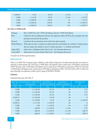
Solved Case Study
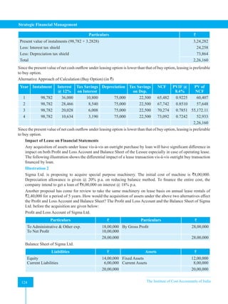
A large profit-making company is considering the installation of a machine to process the waste produced by one of
its existing manufacturing processes to be converted into a marketable product. At present, the waste is removed by
a contractor for disposal on payment by the company of `50 lakhs per annum for the next four year. The contract
can be terminated upon installation of the aforesaid machine on payment of a compensation of `30 lakhs before the
processing operation starts. This compensation is not allowed as deduction for tax purposes.
The machine required for carrying out the processing will cost `200 lakhs to be financed by a loan repayable in 4
equal instalments commencing from the end of year 1. The interest rate is 16% per annum. At the end of the 4th
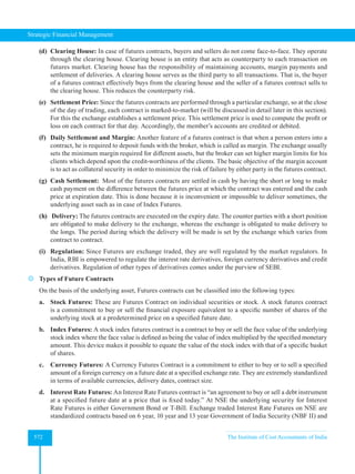
year, the machine can be sold for `20 lakhs and the cost of dismantling and removal will be `15 lakhs.](https://image.slidesharecdn.com/strategyfamous-230209132502-a14bc8e7/85/Strategy_Famous-pdf-73-320.jpg)


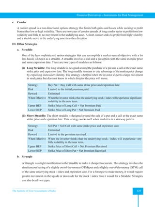
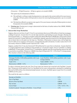
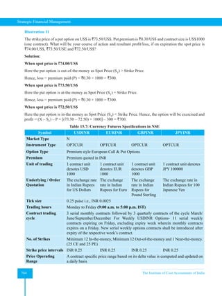
![The Institute of Cost Accountants of India 67
Investment Decisions, Project Planning and Control
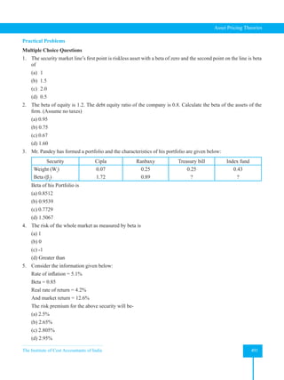
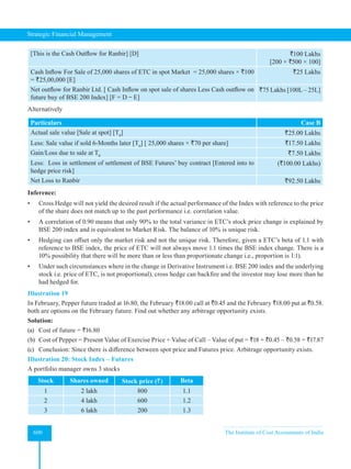
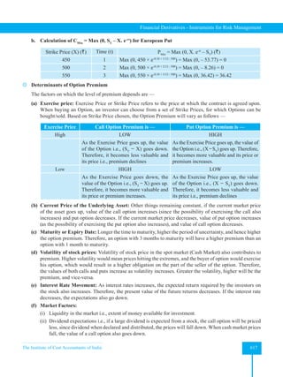
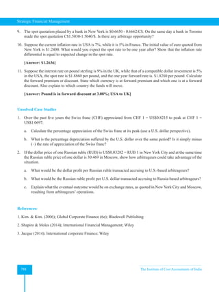
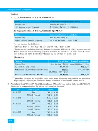
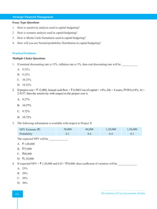
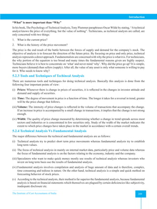
4. The IRR of a project is 10%. If the annual cash flow after tax is `1,30,000 and project duration is 4 years, what
is the initial investment in the project?
A. ` 4,10,000
B. ` 4,12,100
C. ` 3,90,000
D. ` 4,05,000
5. The NPV of a 4-year project is ` 220 lakh and PVIFA at 12% for 4 years is 3.037. The Equivalent Annual
Benefit of the project is ___________
A. ` 66.52 lakh
B. ` 94.74lakh
C. ` 66.96 lakh
D. ` 76.65 lakh
Answer:
1 2 3 4 5
B C A B A
Comprehensive Numerical Problems
1. An oil company proposes to install a pipeline for transport of crude from wells to refinery. Investments and
operating costs of the pipeline vary for different sizes of pipelines (diameter). The following details have been
conducted:
(a) Pipeline diameter (in inches) 3 4 5 6 7
(b) Investment required (` lakhs) 16 24 36 64 150
(c) Gross annual savings in operating costs before depreciation (` lakhs) 5 8 15 30 50
The estimated life of the installation is 10 years. The oil company’s tax rate is 50%. There is no salvage value
and straight-line rate of depreciation is followed.
Calculate the net savings after tax and cash flow generation and recommend therefrom, the largest pipeline to
be installed, if the company desires a 15% post-tax return. Also indicate which pipeline will have the shortest
payback. The annuity PV factor at 15% for 10 years is 5.019.
[Answer: Pipeline diameter of 6 inches has shortest payback period; Pipeline of 6 inches
diameter has highest NPV and it is recommended for installation]](https://image.slidesharecdn.com/strategyfamous-230209132502-a14bc8e7/85/Strategy_Famous-pdf-79-320.jpg)
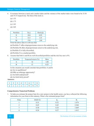
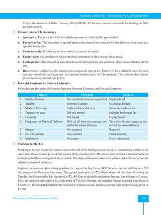
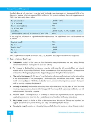
![Strategic Financial Management
68 The Institute of Cost Accountants of India
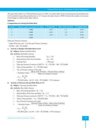
2. A particular project has a four-year life with yearly projected net profit of `10,000 after charging yearly
depreciation of ` 8,000 in order to write-off the capital cost of `32,000. Out of the capital cost `20,000 is
payable immediately (Year 0) arid balance in the next year (which will be the year 1 for evaluation). Stock
amounting to `6,000 (to be invested in year 0) will be required throughout the project and for debtors a further
sum of `8,000 will have to be invested in year 1. The working capital will be recouped in year 5. It is expected
that the machinery will fetch a residual value of `2,000 at the end of 4th year. Income tax is payable @ 40%
and the Depreciation equals the taxation writing down allowances of 25% per annum. Income tax is paid after
9 months after the end of the year when profit is made. The residual value of `2,000 will also bear tax @ 40%.
Although the project is for 4 years, for computation of tax and realisation of working capital, the computation
will be required up to 5 years.
Taking discount factor of 10%, calculate NPV of the project and give your comments regarding its acceptability.
[Answer: NPV = `10,910; Proposal should be accepted]
3. A company is considering a cost saving project. This involves purchasing a machine costing `7,000, which
will result in annual savings on wage costs of `1,000 and on material costs of `400.
The following forecasts are made of the rates of inflation each year for the next 5 years:
Wages costs 10%, Material costs 5%, General prices 6%
The cost of capital of the company, in monetary terms, is 15%.
Evaluate the project, assuming that the machine has a life of 5 years and no scrap value.
[Answer: NPV = (-) `1,067]
4. A Ltd. is considering the question of taking up a new project which requires an investment of `200 lakhs on
machinery and other assets. The project is expected to yield the following gross profits (before depreciation
and tax) over the next five years: (` lakhs)
Year 1 2 3 4 5
Gross profit 80 80 90 90 75
The cost of raising the additional capital is 12% and the assets have to be depreciated at 20% on ‘written
down value’ basis. The scrap value at the end of the five-year period may be taken as zero. Income-tax
applicable to the company is 50%.
Calculate the net present value of the project and advise the management whether the project has to be
implemented. Also calculate the Internal Rate of Return of the project.
[Answer: NPV = `19.31 lakhs; IRR = 15.6%]
5. United Industries Ltd. has an investment budget of `100 lakhs for 2021-22. It has short listed two projects A
and B after completing the market and technical appraisals. The management wants to complete the financial
appraisal before making the investment. Further particulars regarding the two projects are given below:](https://image.slidesharecdn.com/strategyfamous-230209132502-a14bc8e7/85/Strategy_Famous-pdf-80-320.jpg)
![The Institute of Cost Accountants of India 69
Investment Decisions, Project Planning and Control
(` lakhs)
Particulars A B
Investment required
Average annual cash inflow before depreciation and tax (estimate)
100
28
90
24
Salvage value - Nil for both projects.
Estimate life - 10 years for both projects.
The company follows straight line method of charging depreciation. Its tax rate is 50%. You are required to
calculate: (a) Payback period and (b) I.R.R. of the two projects.
[Answer: Payback period = 5.26 years and 5.45 years; IRR = 13.78% and 12.87%]
6. Swastik Ltd. manufacturers of special purpose machine tools, have two divisions which are periodically
assisted by visiting teams of consultants. The management is worried about the steady increase of expense in
this regard over the years. An analysis of last year’s expenses reveals the following: (`)
Consultants’ remuneration
Travel and conveyance
Accommodation expenses
Boarding charges
Special allowances
2,50,000
1,50,000
6,00,000
2,00,000
50,000
12,50,000
The management estimates accommodation expenses to increase by `2,00,000 annually.
As part of a cost reduction drive, Swastik Ltd. are proposing to construct a consultancy centre to take care of
the accommodation requirements of the consultants. This centre will additionally save the company `50,000
in boarding charges and `2,00,000 in the cost of Executive Training Programmes hitherto conducted outside
the company’s premises every year.
The following details are available regarding the construction and maintenance of the new centre:
(a) Land at a cost of `8,00,000 already owned by the company, will be used.
(b) Construction cost `15,00,000 including special furnishings.
(c) Cost of annual maintenance `1,50,000.
(d) Construction cost will be written off over 5 years being the useful life.
Assuming that the write-off of construction cost as aforesaid will be accepted for tax purposes, that the rate
of tax will be 50% and that the desired rate of return is 15%, you are required to analyse the feasibility of the
proposal and make recommendations. The relevant Present Value Factors are:
Year 1 2 3 4 5
PV Factor 0.87 0.76 0.66 0.57 0.50
[Answer: NPV = `10.95 lakhs]](https://image.slidesharecdn.com/strategyfamous-230209132502-a14bc8e7/85/Strategy_Famous-pdf-81-320.jpg)
![Strategic Financial Management
70 The Institute of Cost Accountants of India
7. GFM produces two products - a main product Cp and a co-product Dg. For their main product Cp there is a
100% buy back arrangement with their foreign collaborators. Recently GFM doubled their capacity and with
this their production capacity for the co-product Dg increased to 10,000 MT per annum. Fortunately, there was
an unprecedented increase in demand for Dg and price too has increased significantly to `1,000 per tonne.
However, with delicensing and liberalisation, more and more units for manufacturing Cp and Dg are being set
up in the country. GFM, therefore, anticipates stiff competition for Dg from next financial year. For maintaining
sales at current level (i.e., 10,000 MT per year) GFM will have to drop the price by `50 per MT every year for
the next 5 years when prices are likely to stabilise at pre-boom level of `750 per MT.
The Vice-President (Marketing) who, sensing this situation, has just completed a market study, suggests that
the Company revive and earlier project for converting Dg into Dp grade and starting with 1,000 MT from
next year increase production of Dp in stages of 1,000 MT every year by correspondingly reducing Dg. The
Production Manger estimates that the additional variable cost for Dp will be `200 per MT. V.P. (Marketing)
feels that Dp can be sold at `1,500 per MT but in the first two years a discounted price of `1,400 in year 1
and `1,450 in year 2 will have to be fixed. With partial conversion into Dp, the drop in price of Dg can also
be contained at `25 MT instead of `50 envisaged. Production facilities for Dp involves a capital outlay of `50
lakhs.
Present the projected sales volume and price of products Dg and Dp for the next 5 years under two alternatives.
If GFM normally appraises investments @ 12% p.a. and if cash beyond 5 years from investment are ignored
advise whether Dp should be produced.
[Answer: NPV of incremental cashflow = `12.03 lakhs; conversion of Dg into Dp is advisable.]
8. Electromatic Excellers Ltd. specialise in the manufacture of novel transistors. They have recently developed
technology to design a new radio transistor capable of being used as an emergency lamp also. They are quite
confident of selling all the 8,000 units that they would be making in a year. The capital equipment that would
be required will cost `25 lakhs. It will have an economic life of 4 years and no significant terminal salvage
value.
During each of the first four years promotional expenses are planned as under:
1st Year 1 2 3 4
Advertisement (`) 1,00,000 75,000 60,000 30,000
Others (`) 50,000 75,000 90,000 1,20,000
Variable cost of production and selling expenses: `250 per unit
Additional fixed operating costs incurred because of this new product are budgeted at `75,000 per year.
The company’s profit goals call for a discounted rate of return of 15% after taxes on investments on new
products. The income tax rate on an average works out to 40%. You can assume that the straight-line method
of depreciation will be used for tax and reporting.](https://image.slidesharecdn.com/strategyfamous-230209132502-a14bc8e7/85/Strategy_Famous-pdf-82-320.jpg)
![Strategic Financial Management
72 The Institute of Cost Accountants of India
(4) B Ltd. allocates its head office fixed costs to all products at the rate of `1.25 per direct labour hour. Total
head office fixed costs would not be affected by the introduction of the Product A to the company’s range of
products.
The cost of capital of B Ltd. is estimated at 5% p.a. in real terms and you may assume that all costs and prices
given above will remain constant in real terms. All cash flows would arise at the end of each year, with the
exception of the cost of the machine which would be payable immediately.
The management of B Ltd. is very confident about the accuracy of all the estimates given above, with the
exception of those relating to product life, the annual sales volume and material cost per unit of Product A.
You are required to:
(i) Decide whether B Ltd. should proceed with manufacture of the Product A.
(it) Prepare a statement showing how sensitive the NPV of manufacturing Product A is to errors of estimation
in each of the three factors: Product life. Annual Sales Volume and Material cost per unit of Product A.
Ignore taxation.
The present value of annuity for 3 years, 4 years and 5 years at 5% respectively are 2.72, 3.55 and 4.33.
[Answer: NPV = `1,26,710; So, product A is recommended; Sensitivity forecast error: Product
life = 3.2 years i.e., 36% lower limit of error; Annual sales volume =7074 units i.e., 29% lower
limit and Material cost A = `7,426 i.e., 65% upper limit].
References:
1. Pandey, I M; Essentials of Financial Management; Pearson Publication
2. Chandra, P.; Financial Management – Theory and Practice; McGraw Hill
3. Khan and Jain; Financial Management – Text, Problems and Cases; McGraw Hill
4. Brigham and Houston; Fundamentals of Financial management; Cengage](https://image.slidesharecdn.com/strategyfamous-230209132502-a14bc8e7/85/Strategy_Famous-pdf-84-320.jpg)
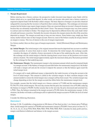
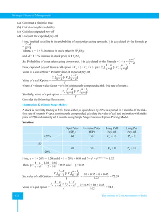
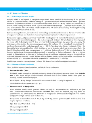
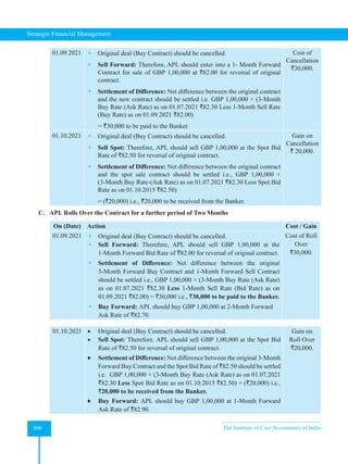
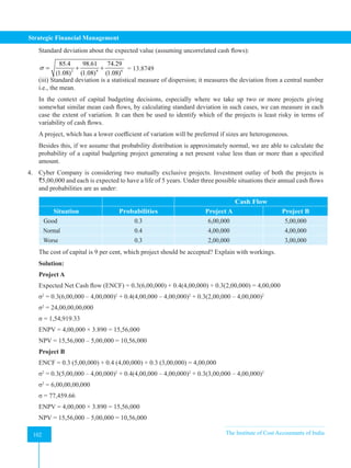
![Strategic Financial Management
82 The Institute of Cost Accountants of India
82
Solution:
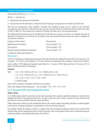
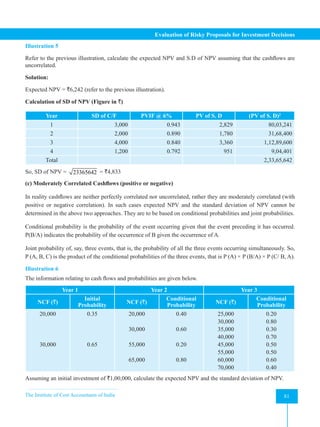
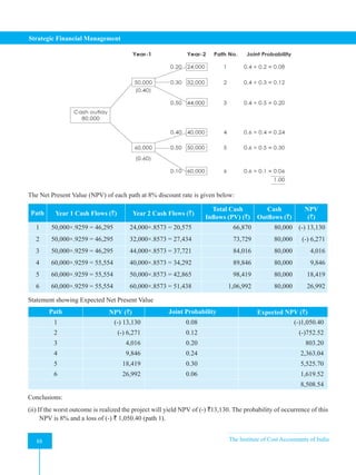
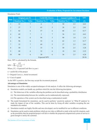
Here, we need to calculate the joint probabilities associated with each possible stream of cashflows as follows:
(Figure in `)
Year 1 Year 2 Year 3 Joint
Probabil-
ity
NCF (`) Initial
Probability
NCF (`) Conditional
Probability
NCF (`) Conditional
Probability
20,000
30,000
0.35
0.65
20,000
30,000
55,000
65,000
0.40
0.60
0.20
0.80
25,000
30,000
35,000
40,000
45,000
55,000
60,000
70,000
0.20
0.80
0.30
0.70
0.50
0.50
0.60
0.40
0.028*
0.112
0.063
0.147
0.065
0.065
0.312
0.208
*0.028 = 0.35 × 0.40 × 0.20 [cash flow `20,000(1st
year) – `20,000 (2nd
year) – `25,000 (3rd
year)]
Cash
Flow
Stream
NPV
Joint
Probability
NPV × Joint
Prob.
(NPV – Exp.
NPV)2
× Joint
Prob.
1.
1 2 3
20000 20000 25000
(1.06) (1.06) (1.06)
+ + – 100000 = - 42340
0.028 -1185.52 96005724
2.
1 2 3
20000 20000 30000
(1.06) (1.06) (1.06)
+ + – 100000 = - 38340
0.112 -4271.68 333348944
3.
1 2 3
20000 30000 35000
(1.06) (1.06) (1.06)
+ + – 100000 = - 25040
0.063 -1577.52 107228325
4.
1 2 3
20000 30000 40000
(1.06) (1.06) (1.06)
+ + – 100000 = - 20840
0.147 -3063.48 201849905
5.
1 2 3
30000 55000 45000
(1.06) (1.06) (1.06)
+ + – 100000 = 19755
0.065 1284.075 814208.887
6.
1 2 3
30000 55000 55000
(1.06) (1.06) (1.06)
+ + – 100000 = 28155
0.065 1830.075 9265469.89
7.
1 2 3
30000 65000 60000
(1.06) (1.06) (1.06)
+ + – 100000 = 41255
0.312 12871.56 195612781
8.
1 2 3
30000 65000 70000
(1.06) (1.06) (1.06)
+ + – 100000 = 49655
0.208 10328.24 232582156
Total Exp. NVP 16215.75 1174267896
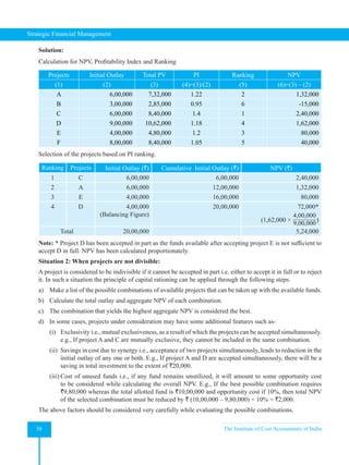
Expected NPV = `16,215.75
S.D of NPV = 1174267896 = `34,268](https://image.slidesharecdn.com/strategyfamous-230209132502-a14bc8e7/85/Strategy_Famous-pdf-94-320.jpg)
![Strategic Financial Management
84 The Institute of Cost Accountants of India
84
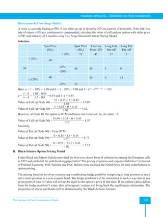
Illustration 8
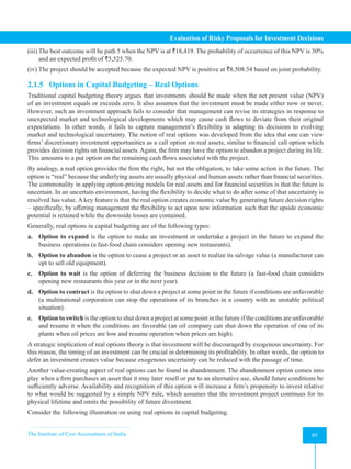
Refer to our previous illustration no. 6. Suppose, we are interested to calculate the probability that NPV of the
project will be at least `20,000. The same can be calculated as follows
Solution:
P (NPV ≥ 50000) = P
NPV - Expected NPV 20000 16215.75
S.D of NPV 34268
−
≥
= P (Z ≥ 0.11) = 1 -
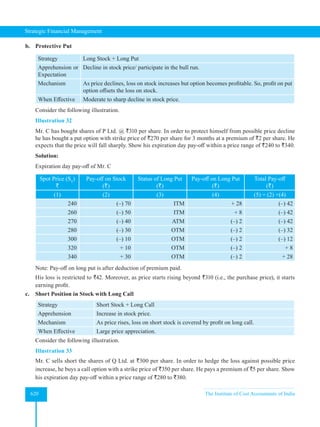
Profit
P/V Ratio (0.11)
= 1 – (0.5 +0.4602) = 0.0398 = 3.98%
Note: For
Profit
P/V Ratio
(0.11), please refer to standard normal distribution table.
Illustration 9
A project has expected NPV value of `800 and S.D. of NPV of `400. The management wants to determine the
probability of the NPV under the following ranges.
(i) Zero or less
(ii) Greater than zero
(iii) Between the range of `500 and `900
(iv) Between the range of `300 and `600
Solution:
(i) P (NPV ≤ 0)
=
NPV- expected NPV 0 800
P
S.D. of NPV 400
−
≤
= P (Z ≤ - 2) = (-2) = 1 – (2) = 1- (0.50 + 0.4772) = 0.0228 or 2.28%
(ii) P (NPV ≥ 0)
=
NPV- expected NPV 0 800
P
S.D. of NPV 400
−
≥
= P (Z ≥ - 2) =1 - P (Z ≤ - 2) = 1-
Profit
P/V Ratio
(-2) =
Profit
P/V Ratio
(2) = (0.50 + 0.4772) = 0.9772 or 97.72%
(iii) When NPV = 500; Z = (500 – 800) / 400 = - 300/400 = - 3/ 4 = - 0.75
When NPV = 900; Z = (900 – 800) / 400 = 100/400 = 1/ 4 = 0.25
Table Value of 0.75 = .2734 and 0.25 = .0987; so,
Profit
P/V Ratio
(0.25) = 0.5987 and
Profit
P/V Ratio
(0.75) = 0.7734
P (NPV between 500 & 900)
= P (500 ≤ NPV ≤ 800)
= P (-0.75 ≤ Z ≤ 0.25)
=
Profit
P/V Ratio
(0.25) - (-0.75)
=
Profit
P/V Ratio
(0.25) – [1- (0.75)]
= 0.5987 – [1 – 0.7734]
= 0.5987 – 0.2266 = 0.3721 = 37.21%](https://image.slidesharecdn.com/strategyfamous-230209132502-a14bc8e7/85/Strategy_Famous-pdf-96-320.jpg)
![The Institute of Cost Accountants of India 85
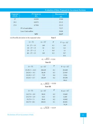
Evaluation of Risky Proposals for Investment Decisions
(iv) Table Value of 1.25 = 0.3944 and 0.50 = 0.1915; so,
Profit
P/V Ratio
(1.25) = 0.8944 and
Profit
P/V Ratio
(0.50) = 0.6915
P (NPV between 300 & 600)
= P (300 ≤ NPV ≤ 600)
= P (-1.25 ≤ Z ≤ -0.50)
=
Profit
P/V Ratio
(-0.5) -
Profit
P/V Ratio
(-1.25)
= [1-
Profit
P/V Ratio
(0.5)] – [1-
Profit
P/V Ratio
(1.25)]
= 0.3085 – 0.1056
= 0.2029 = 20.29%
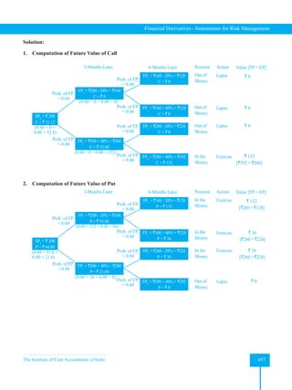
2.1.4 Decision Tree Analysis
Decision Tree Analysis is a useful tool for analysis of investment proposals incorporating project flexibility. The
decision-tree method analyses investment opportunities involving a sequence of decisions over time. Various
decision points are defined in relation to subsequent chance events. The Expected NPV for each decision point
is computed based on the series of NPVs and their probabilities that branch out or follow the decision point in
question. In other words, once the range of possible decisions and chance events are laid out in tree-diagram form,
the NPVs associated with each decision are computed by working backwards on the diagram from the expected
cash flows defined for each path on the diagram. The optimal decision path is chosen by selecting the highest
expected NPV.
The following is an illustration on a decision tree relating to an investment proposal.
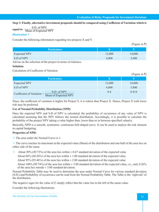
Illustration 10
A firm has an investment proposal, requiring an outlay of `40,000. The investment proposal is expected to have
2 years’ economic life with no salvage value. In year 1, there is a 0.4 probability that cash inflow after tax will be
`25,000 and 0.6 probability that cash inflow after tax will be `30,000. The probabilities assigned to cash inflows
after tax for the year 2 are as follows:
The Cash inflow year 1 ` 25,000 `30,000
The Cash inflow year 2 Probability Probability
` 12,000 0.2 ` 20,000 0.4
` 16,000 0.3 ` 25,000 0.5
` 22,000 0.5 ` 30,000 0.1
The firm uses a 12% discount rate for this type of investment.
Required:
(i) Construct a decision tree for the proposed investment project.
(ii) What net present value will the project yield if worst outcome is realized? What is the probability of occurrence
of this NPV?
(iii)What will be the best and the probability of that occurrence?
(iv)Will the project be accepted?](https://image.slidesharecdn.com/strategyfamous-230209132502-a14bc8e7/85/Strategy_Famous-pdf-97-320.jpg)
![Strategic Financial Management
92 The Institute of Cost Accountants of India
92
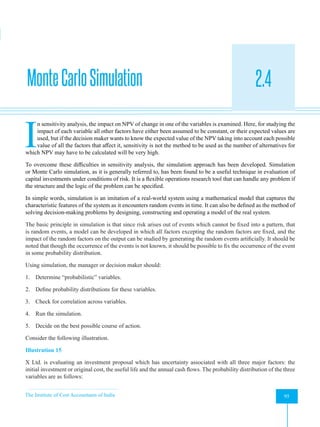
Investment: Let the investment be ` X
- X + 50000 (0.909 + 0.826 + 0.751) = 0
X = 50000 (0.909 + 0.826 + 0.751) = 1,24,300
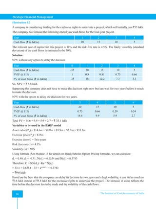
So, the investment can be as high as `1,24,300 before the appraisal advice to invest becomes incorrect. In other
words, if the original estimate increases by more than `24,300 or 24.30%, the NPV will be negative.
Life: Let the life be X years.
- 100000 + 50000 × PVIFA (10%, X) = 0
PVIFA (10%, x) = 100000 / 50000 = 2
Now, PVIFA (10%, 2) = 1.74 and PVIFA (10%, 3) = 2.49 [ i.e., (0.909 + 0.826 + 0.751)]
Using simple interpolation, we get X = 2.35 years.
So, if the life of the asset decreases by more than 0.65 years or 21.67%, the NPV will be negative.
Net Cash Flow (NCF): Let the annual NCF be ` X
- 100000 + X (0.909 + 0.826 + 0.751) = 0
or, 2.486 X = 100000
or, X = 100000/2.486 = 40225
Decrease in NCF that can be tolerated = 50,000 – 40225 = ` 9,775
Percentage change = (9775/50,000) × 100 = 19.55%
So, if the NCF decreases by more than 9775 or 19.55%, the NPV will be negative
Discount Rate: Let the discount rate be X%
-100000 + 50000 × PVIFA (X%, 3) = 0
PVIFA (X%, 3) = 100000 / 50000 = 2
From Table,
PVIFA (20%, 3) = 2.11 and PVIFA (25%, 3) = 1.95
Using simple interpolation, we get, X = 0.234 or 23.4%
Discount rate can be increased from 10% to 23.4% or it can tolerate an increase of 134% in discount rate before
NPV becomes zero.
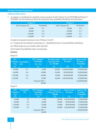
The summarized result of the sensitivity analysis is shown below:
Element or Variable Sensitivity
Initial Investment 24.30%
Net Cash Inflow 19.55%
Life 21.67%
Discount Rate 23.40%](https://image.slidesharecdn.com/strategyfamous-230209132502-a14bc8e7/85/Strategy_Famous-pdf-104-320.jpg)
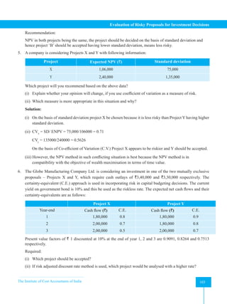
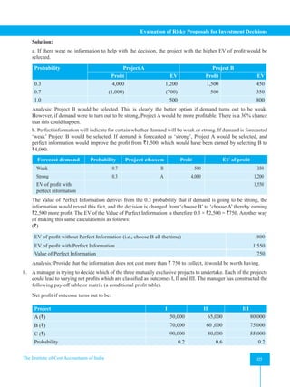
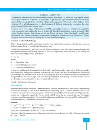
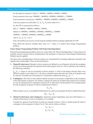
![The Institute of Cost Accountants of India 107
Evaluation of Risky Proposals for Investment Decisions
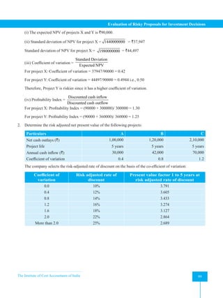
Outcome
Project
A B C
I (Worst) [90,000 – 50,000] = 40,000 [90,000 – 70,000] = 20,000 [90,000 – 90,000] = 0
II (Most likely) [1,00,000 - 85,000] = 15,000 [1,00,000 - 75,000] = 25,000 [1,00,000 – 1,00,000] = 0
III (Best) [1,40,000 - 1,30,000]=10,000 [1,40,000 – 1,40,000] = 0 [1,40,000 –
1,10,000]=30,000
Analysis: The maximum regret is 40,000 with project A, 25,000 with B and 30,000 with C. The lowest of these
three maximum regrets is 25,000 with B, and so project B would be selected if the minimax regret rule is used.
Note: The minimax regret rule aims to minimize the regret from making the wrong decision. Regret is the
opportunity lost through making the wrong decision.
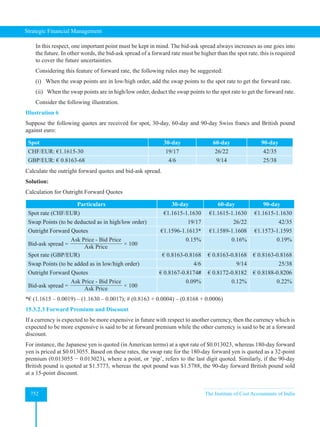
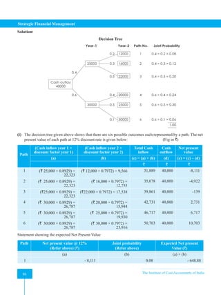
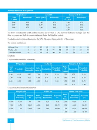
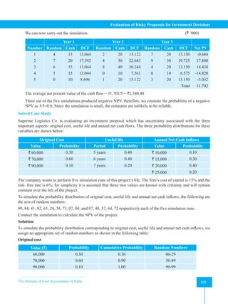
10. Infoway Ltd. is considering the purchase of an automatic packing machine to replace the 2 machines which are
currently used to pack Product X. The new machine would result in reduced labour costs because of the more
automated nature of the process and in addition, would permit production levels to be increased by creating
greater capacity at the packing stage with an anticipated rise in the demand for Product X, it has been estimated
that the new machine will lead to increased profits in each of the next 3 years. Due to uncertainty in demand
however, the annual cash flows (including savings) resulting from purchase of the new machine cannot be
fixed with certainty and have therefore, been estimated probabilistically as follows:
Annual cashflows: (` ‘000)
Year 1 Probability Year 2 Probability Year 3 Probability
10 0.3 10 0.1 10 0.3
15 0.4 20 0.2 20 0.5
20 0.3 30 0.4 30 0.2
40 0.3
Due to the overall uncertainty in the sales of Product X, it has been decided that only 3 years cash flows will be
considered in deciding whether to purchase the new machine. After allowing for the scrap value of the existing
machines, the net cost of the new machine will be `42,000. The effects of taxation should be ignored.
Required:
(a) Ignoring the time value of money, identify which combinations of annual cash flows will lead to an overall
negative net cash flow, and determine the total probability of this occurring.
(b) On the basis of the average cash flow for each year, calculate the net present value of the new machine
given that the company’s cost of capital is 15%. Relevant discount factors are as follows:
Year Discount factor
1 0.8696
2 0.7561
3. 0.6575
(c) Analyse the risk inherent in this situation by simulating the net present value calculation. You should
use the random number given at the end of the illustration in 5 sets of cash flows. On the basis of your
simulation results what is the expected net present value and what is the probability of the new machine
yielding a negative net present value?](https://image.slidesharecdn.com/strategyfamous-230209132502-a14bc8e7/85/Strategy_Famous-pdf-119-320.jpg)
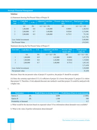
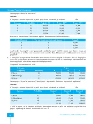
![Strategic Financial Management
108 The Institute of Cost Accountants of India
108
Set 1 Set 2 Set 3 Set 4 Set 5
Year 1 4 7 6 5 0
Year 2 2 4 8 0 1
Year 3 7 9 4 0 3
Solution:
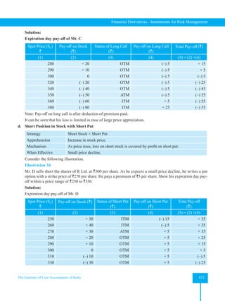
(a) If the total cash flow in years 1, 2 and 3 is less than `42,000, the net cash flow will be negative. The
combinations of cash flow with total less than `42,000 are given in table below:
Cash flow (`’000)
Year 1 Probability Year 2 Probability Year 3 Probability Total Joint Probability
10 0.3 10 0.1 10 0.3 30 0.3 × 0.1 × 0.3 = 0.009
10 0.3 10 0.1 20 0.5 40 0.3 × 0.1 × 0.5 = 0.015
10 0.3 20 0.2 10 0.3 40 0.3 × 0.2 × 0.3 = 0.018
15 0.4 10 0.1 10 0.3 35 0.4 × 0.1 × 0.3 = 0.012
20 0.3 10 0.1 10 0.3 40 0.3 × 0.1 × 0.3 = 0.009
Total = 0.063
The probability of a negative cash flow is 0.063
(b) Expected cash flow = Σ [Cash flow × Probability]
(`’000)
Year 1 EV = (10×0.3) + (15×0.4) + (20×0.3) 15
Year 2 EV = (10×0.1) + (20×0.2) + (30×0.4) + (40×0.3) 29
Year 3 EV = (10×0.3) + (20×0.5) + (30×0.2) 19
P.V. of the cash = (15×0.8696) + (29×0.7561) + (19×0.6575) = `47,463
The net present value of the new machine = 47,463 – 42,000 = `5,463
(c) Allocated random number ranges to the cash flows for each year.
Cashflow (` 000) Probability Random number
Year 1 10 0.3 0 - 2
15 0.4 3 - 6
20 0.3 7 - 9
Year 2 10 0.1 0
20 0.2 1 - 2
30 0.4 3 - 6
40 0.3 7 - 9
Year 3 10 0.3 0 - 2
20 0.5 3 - 7
30 0.2 8 - 9](https://image.slidesharecdn.com/strategyfamous-230209132502-a14bc8e7/85/Strategy_Famous-pdf-120-320.jpg)
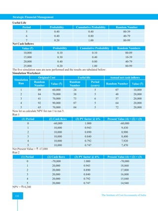

![The Institute of Cost Accountants of India 115
Evaluation of Risky Proposals for Investment Decisions
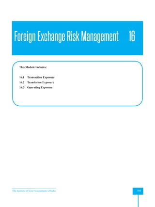
5. Given, expected value of profit without perfect information = `1,600 and expected value of perfect information
= `300, then expected value of profit with perfect information will be ________
A. `1,300
B. `1,900
C. `950
D. None of the above
Answer:
1 2 3 4 5
A A C A B
Comprehensive Numerical Problems
1. Diamond industries is considering investment in specialized moulds which cost `1.00 lakh, with a life of 2
years, after which there is no expected value. The possible incremental cash flows (post-tax) are:
Year I Year II
Cash flow (`) Probability Cash flow (`) Probability
60,000 0.20 50,000 0.20
70,000 0.50 60,000 0.50
80,000 0.30 70,000 0.30
The risk-free rate of return required by the company is 10%.
Required:
a. Assume that the cash flows are perfectly correlated. Calculate the expected net present value and the
standard deviation of the net present value of the probability distribution of possible net present values.
b. If the NPV were normally distributed what is the probability of the investment providing a negative net
present value?
c. If the cash flows were independent what would be the probability of the NPV being negative?
[Answer: Expected NPV = `14,958 and S.D = `12,149; 10.93%; 4.09%]
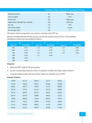
2. Calculate the Expected NPV and S.D (NPV) for the moderately correlated cash flows which are expected to be
generated by a certain project which are shown in the table below
Year 1 Year 2 Year 3
Net cash flow
(`)
Initial
probability
Net cash flow (`) Probability
Net cash flow
(`)
Probability
50,000 0.6 50,000 0.8 40,000 0.70
35,000 0.30
75,000 0.2 80,000 0.50](https://image.slidesharecdn.com/strategyfamous-230209132502-a14bc8e7/85/Strategy_Famous-pdf-127-320.jpg)
![Strategic Financial Management
116 The Institute of Cost Accountants of India
116
70,000 0.50
80,000 0.4 85,000 0.6 85,000 0.60
95,000 0.40
1,10,000 0.4 1,05,000 0.35
1,15,000 0.65
The initial outlay for the project is `1,50,000 and the risk-free interest rate is 6%.
[Answer: `27,667; `56,807]
3. Rama Chemicals is considering an investment project. The estimated life of the project is 3 years. The cost of
the project is `15,000. The projected cash flows are given below.
Year 1 Year 2 Year 3
Net cash flow (`)
Initial
probability
Net cash flow (`) Probability Net cash flow (`) Probability
6,000 0.3 4,00 0.2 6,000 0,3
5,000 0.4 6,000 0.6 10.000 0.4
14,000 0.3 12,000 0.2 14,000 0.3
The cash flows are independent and the post-tax risk-free discount rate is 6%. You are required to analyze the
project for Rama Chemicals.
Required:
a. Calculate the expected net present value.
b. Calculate the probability of NPV being zero or less.
[Answer: `6,995; 8.85%]
4. A company is trying to choose between two investment proposals A and B. Project A has a standard deviation
of `6,500 while Project B has a standard deviation of `7,200. The finance manager wishes to know which
investment to choose, given each of the following combinations of the expected values;
(i) Project A and Project B both have expected net present value of `15,000. (ii) Project A has expected NPV of
`18,000 while for Project B it is `22,000.
[Answer: (i) Since expected NPV are similar, the project with lower S.D is recommended (i.e., Project
A); COV for Project A 0.361 and for B 0.327 and hence Project B is recommended]
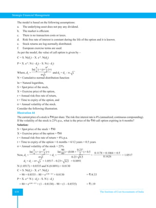
5. From the following project details calculate the sensitivity of the (a) Project cost, (b) Annual cash flow, and (c)
Cost of capital. Which variable is the most sensitive?
Project cost ` 12,000 Annual cash flow ` 4,500
Life of the project 4 years Cost of capital 14%
The annuity factor at 14% for 4 years is 2.9137 and at 18% for 4 years is 2.6667.
[Answer: (a) 9.27%; (b) 8.48%; (c) 29%]
Unsolved Case Study
Trabco Cables is considering the risk characteristics of a project. The firm has identified that the following factors
have a bearing on the NPV of the project which are not subject to much variation and may be deemed to be constant
at the following levels:](https://image.slidesharecdn.com/strategyfamous-230209132502-a14bc8e7/85/Strategy_Famous-pdf-128-320.jpg)


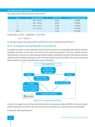
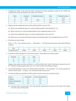
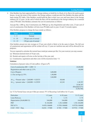
![The Institute of Cost Accountants of India 137
Leasing Decisions
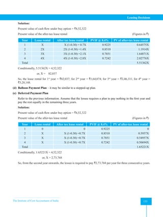
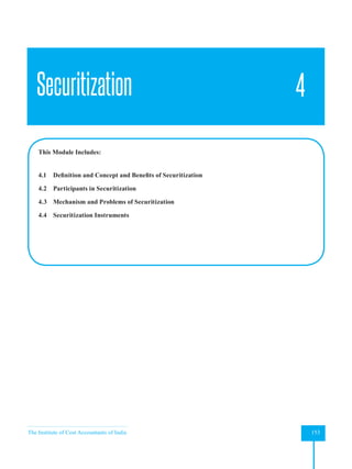
Comment: The present value of net cash flows is lowest for lease option; hence it is suggested to take
equipment on lease basis.
2. Fair finance, a leasing company, has been approached by a prospective customer intending to acquire a machine
whose Cash Down price is `3 crores. The customer, in order to leverage his tax position, has requested a quote
for a three-year lease with rentals payable at the end of each year but in a diminishing manner such that they
are in the ratio of 3: 2: 1. Depreciation can be assumed to be on straight line basis and Fair Finance’s marginal
tax rate is 35%. The target rate of return for Fair Finance on the transaction is 12%.
Calculate the lease rents to be quoted for the lease for three years.
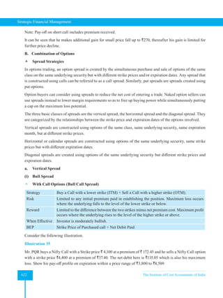
Solution:
Capital sum to be placed under Lease
Particulars ` in lakhs
Cash Down price of machine
Less: PV of depreciation tax shield [100 × 0.35 × PVIFA (12%, 3 years) = 35 × 2.4018]
300.00
84.06
215.94
If the normal annual lease rent per annum is x, then cash flow will be:
Year Post-tax cash flow P.V. of post-tax cash flow
1 3x × (1 – .35) = 1.95x 1.95×(1/1.12) =1.7411x
2 2x × (1 – .35) = 1.3x 1.30 × [(1/(1.12)
2
] = 1.0364x
3 x × (1 – .35) = 0.65x 0.65 × [1/(1.12)
3
] = 0.4626x
= 3.2401x
Therefore 3.2401 x = 215.94
or, x = `66.6409 lakhs
Year-wise rentals are as follows: (` in lakhs)
Year 1 3 × 66.6409 lakhs 199.9227
Year 2 2 × 66.6409 lakhs 133.2818
Year 3 1 × 66.6409 lakhs 66.6409
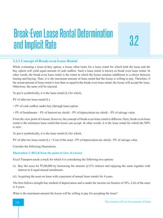
3. ABC Company Ltd. is faced with two options as under in respect of acquisition of an asset valued `1,00,000/-
Either
(a) to acquire the asset directly by taking a Bank Loan of `1,00,000/- repayable in 5 year-end instalments at
an interest of 15%.
OR
(b) to lease in the asset at yearly rentals of `320 per `1,000 of the asset value for 5 years payable at year end.
The following additional information are available.
(a) The rate of depreciation of the asset is 15% W.D.V.
(b) The company has an effective tax rate of 50%.
(c) The company employs a discounting rate of 16%.](https://image.slidesharecdn.com/strategyfamous-230209132502-a14bc8e7/85/Strategy_Famous-pdf-149-320.jpg)
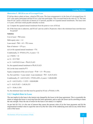
![Strategic Financial Management
140 The Institute of Cost Accountants of India
140
PVCF 3.7908 2.3538 1.4615
PV 2.464X + 217592 1.836X + 135108 1.425X + 83890
Leasing Decision: Total PV = 5.725 X + 436590
P/V of Terminal Cash Inflows: `
Nominal value of flats after 15 years 8,00,000
Less: Tax on Profit [8,00,000 × 35%] 2,80,000
Total 5,20,000
PV = 5,20,000 × 0.239 1,24,280
At 10% Rate of Return: P/V of Cash Inflows = P/V of Cash outflows
5.725X + 4,36,590 + 1,24,280 = 25,90,700
Or, X = 3,54,555.
Lease Rent per Flat = 3,54,555/6 = `59,092.50
5. The Sharda Beverages Ltd has taken a plant on lease, valued at `20 crore. The lease arrangement is in the form
of a leveraged lease. The Kuber Leasing Limited is the equity participant and the Hindusthan Bank Ltd. (HBL)
is the loan participant. They fund the investment in the ratio of 2:8. The loan from HBL carries a fixed rate of
interest of 19 percent, payable in 6 equated annual instalments. ‘The lease term is 6 years, with lease rental
payable annually in arrear.
a) Compute the equated annual instalment from the point or view - of HBL.
b) If the lease rate is unknown, and HBL’s per-tax yield is 25 percent, what is the minimum lease rent that
must be quoted’?
Solution:
Cost of the asset `20 cr
Debt Equity ratio 2: 8
Loan raised (20 × 8/10) = `16cr
Rate of interest 19%
(a) Computation of annual instalment
X × PVCF6yr, 19%
= `16 cr.
X = `16 cr/3.4098
X = 4,69,23,573
So, equated annual instalment is `4,69,23,573
(b) Let the lease rent be X
Net outflow = Lease rent – Loan instalment = X – 46923573
Then,
(X – 46923573) PVCF6yr, 25%
= 40000000
X = 6,04,76,463
Minimum lease rental to be quoted is `6,04,76,463.](https://image.slidesharecdn.com/strategyfamous-230209132502-a14bc8e7/85/Strategy_Famous-pdf-152-320.jpg)


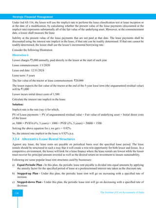
![Strategic Financial Management
150 The Institute of Cost Accountants of India
150
Practical Problems
Comprehensive Practical Problems
1. A firm has the choice of buying a piece of equipment at a cost of `1,00,000 with borrowed funds at a cost of
18% p.a. repayable in five annual instalments of `32,000, or to take on lease the same on an annual rental of
`32,000. The firm is in the tax-bracket of 40%.
Assume:
(i) The salvage value of the equipment at the end of the period is zero.
(ii) The firm uses straight line depreciation.
Discounting factors are:
@ 9% 0.917 0.842 0.772 0.708 0.650
@ 11% 0.901 0.812 0.731 0.659 0.593
@ 18% 0.847 0.718 0.609 0.516 0.437
Which alternative do you recommend?
[Answer: PV of advantage of owning = `1050; Owning is recommended]
2. PQR. Ltd. is considering the possibility of purchasing a multipurpose machine which cost `10 lakhs. The
machine has an expected life of 5 years. The machine generates `6 lakhs per year before depreciation and
tax, and the management wishes to dispose the machine at the end of 5 years which will fetch `1 lakh. The
depreciation allowable for the machine is 25% on written down value and the company’s tax rate is 50%.
The company approached a NBFC for a five-year lease for financing the asset which quoted a rate of `28 per
thousand per month. The company wants you to evaluate the proposal with purchase option. The cost of capital
of the company is 12% and for lease option it wants you to consider a discount rate of 16%.
[Answer: Net Present Value: Purchase option = `4,31,000;
Lease = `4,33,000; Lease is recommended]
3. XYZ Ltd. is considering a proposal to acquire an equipment costing `5,00,000. The expected effective life of
the equipment is 5 years. The company has two options - either to acquire it by obtaining a loan of `5 lakhs at
12% interest p.a. or by lease. The following additional information is available:
(i) the principal amount of loan will be repaid in 5 equal yearly instalments.
(ii) the full cost of the equipment will be written off over a period of 5 years on straight line basis and it is to
be assumed that such depreciation charge will be allowed for tax purpose.
(iii) the effective tax rate for the company is 40% and the after-tax cost of capital is 10%.
(iv) the interest charge, repayment of principal and the lease rentals are to be paid on the last day of each year.
You are required to work out the amount of lease rental to be paid annually, which will match the loan option.
[Answer: Required lease rental is `1,38,277]](https://image.slidesharecdn.com/strategyfamous-230209132502-a14bc8e7/85/Strategy_Famous-pdf-162-320.jpg)
![The Institute of Cost Accountants of India 151
Leasing Decisions
4. Welsh Limited is faced with a decision to purchase or acquire on lease a mini car. The cost of the mini car is
`1,26,965. It has a life of 5 years. The mini car can be obtained on lease by paying equal lease rentals annually.
The leasing company desires a return of 10% on the gross value of the asset. Welsh Limited can also obtain
100% finance from its regular banking channel. The rate of interest will be 15% p.a. and the loan will be paid
in five annual equal instalments, inclusive of interest. The effective tax rate of the company is 40%. For the
purpose of taxation, it is to be assumed that the asset will be written off over a period of 5 years on a straight-
line basis.
(a) Advise Welsh Limited about the method of acquiring the car.
(b) What should be the annual lease rental to be charged by the leasing company to match the loan option?
For your exercise use the following discount factors:
Discount Rate Year 1 Year 2 Year 3 Year 4 Year 5
10% 0.91 0.83 0.75 0.68 0.62
15% 0.87 0.76 0.66 0.57 0.49
9% 0.92 0.84 0.77 0.71 0.65
[Answer: (a) PV of cash outflow under lease = `81,719; under debt financing = `87,335; Lease is
recommended; (b) Required lease rental = `34,906]
5. The FFM Ltd. is in the tax bracket of 35% and discounts its cash flows at 16%. In the acquisition of an asset
worth `10,00,000, it is given two offers - either to acquire the asset by taking a bank loan @ 15% p.a. repayable
in five yearly instalments of `2,00,000 each plus interest or to lease-in the asset at yearly rentals of `3,24,000
for five years. In both cases, the instalment is payable at the end of the year. Applicable rate of depreciation is
15% using ‘written down value’ (WDV) method.
You are required to suggest the better alternative.
[Answer: PV of cash outflow: Under Lease = `6,89,505;
Under Buy = `7,31,540; Leasing is recommended]
Unsolved Case Study
Modern Outlook Ltd. (MOL), a small manufacturing firm, is considering the acquisition of the use of a machine.
After evaluating equipment offered by seven different manufacturers, it has come to the conclusion that ‘Z’ was
the most suitable machine for its needs. Consequently, it has asked the manufacturer’s sales personnel to provide
information on alternative financing plans available through their financing subsidiary. The subsidiary presented
the two alternatives.
Alternative I was to lease the ‘Z’ equipment for 7 years, which was the machine’s expected useful life. The annual
lease payments would be `14,700 and would include service and maintenance. Lease payments would be due at
the beginning of the year. Lease payments would be fully tax-deductible.](https://image.slidesharecdn.com/strategyfamous-230209132502-a14bc8e7/85/Strategy_Famous-pdf-163-320.jpg)
![Strategic Financial Management
152 The Institute of Cost Accountants of India
152
Alternative II would be to purchase the ‘Z’ equipment through 100% loan from the financing subsidiary. The cost
of the machine is `50,000. It would make seven annual payments of `9,935 each to repay the loan of `50,000.
Payments would be, at the end of each year.
The MOL’s marginal tax rate in 44%, It has estimated that the equipment has an expected salvage value of `1,000.
The company plans to depreciate the equipment by using straight-line method. The service and maintenance would
cost `3,700 annually.
You are required to advice MOL on the desirability of the alternative plans, assuming that the rate of interest is
9% p.a.
[Answer: PV of cash outflow: Under Lease = `50,014;
Under Buy = `43,537; Buying is recommended]
References:
1. Pandey, I M; Essentials of Financial Management; Pearson Publication
2. Chandra, P.; Financial Management – Theory and Practice; McGraw Hill
3. Khan and Jain; Financial Management – Text, Problems and Cases; McGraw hill
4. Brigham and Houston; Fundamentals of Financial management; Cengage](https://image.slidesharecdn.com/strategyfamous-230209132502-a14bc8e7/85/Strategy_Famous-pdf-164-320.jpg)
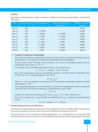
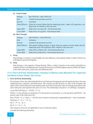
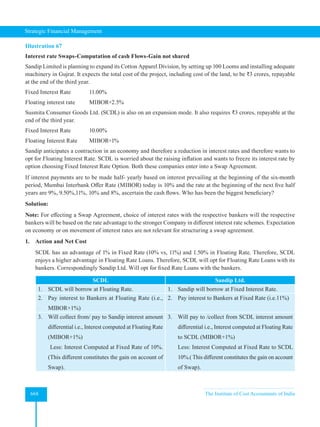
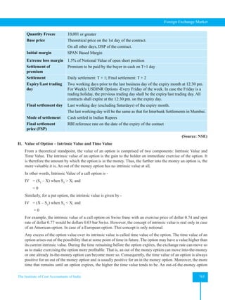
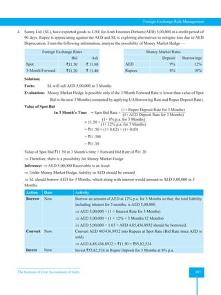
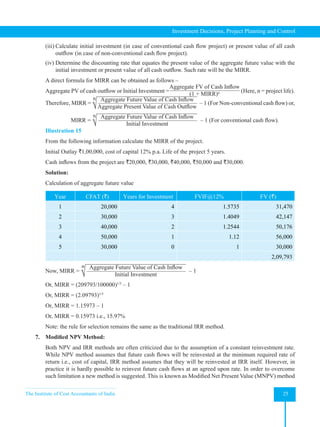
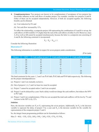
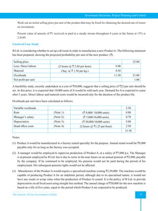
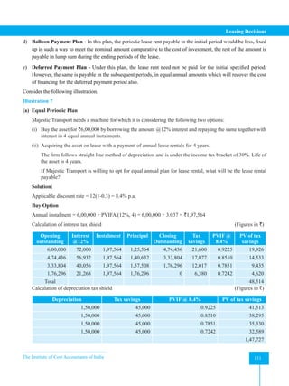
![Strategic Financial Management
160 The Institute of Cost Accountants of India
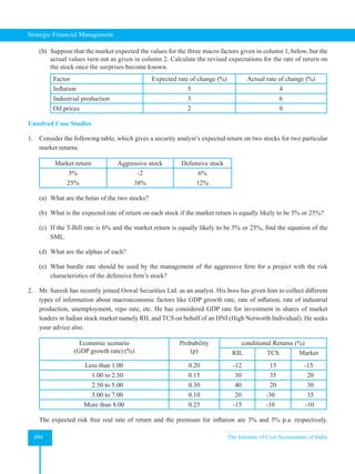
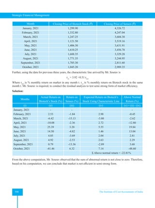
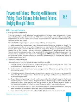
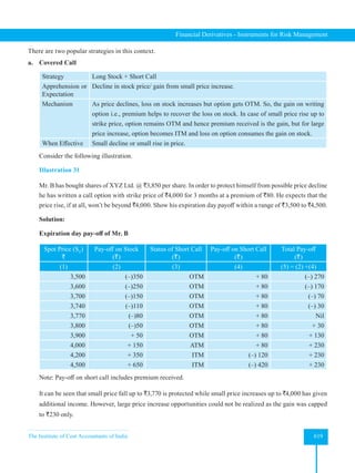
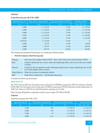
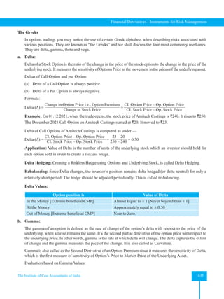
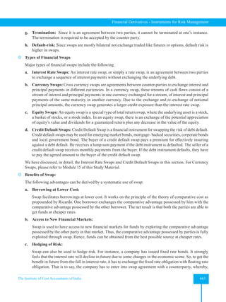
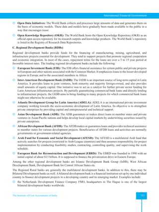
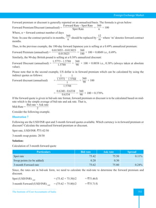
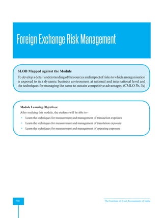
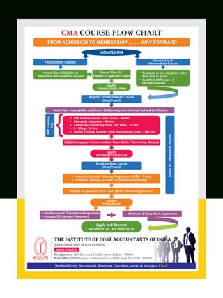
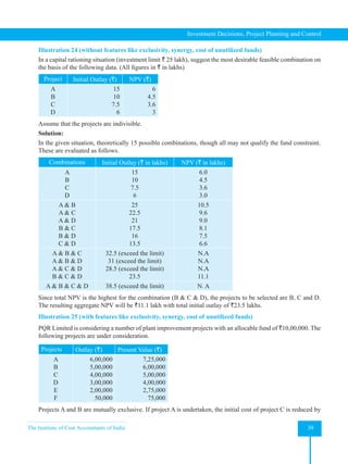
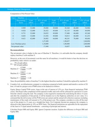
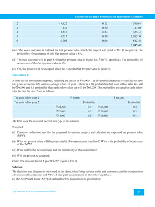
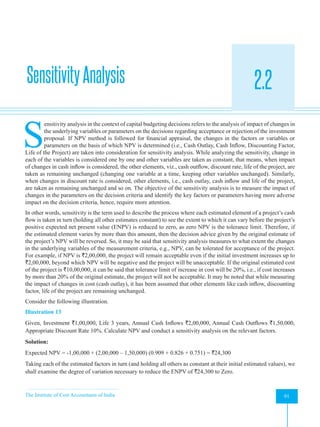
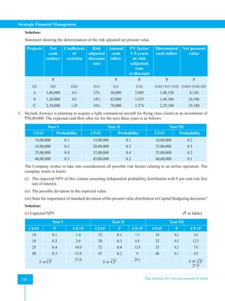
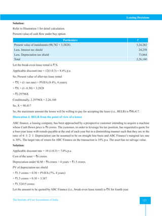
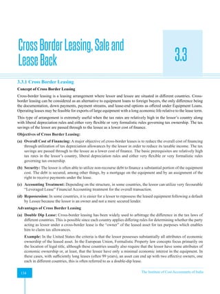
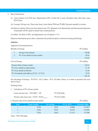
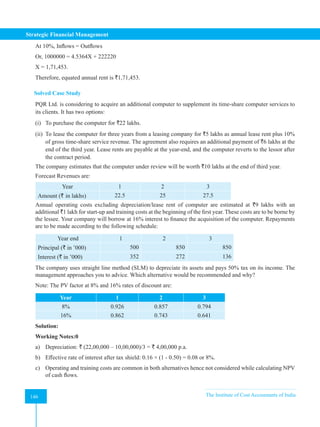
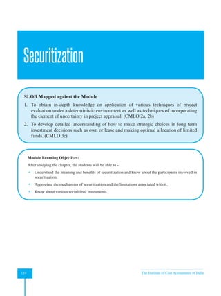
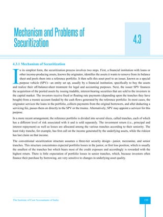
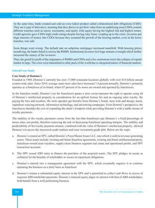
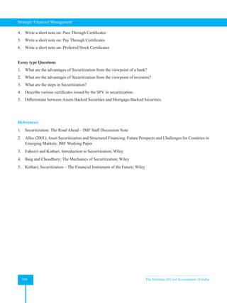
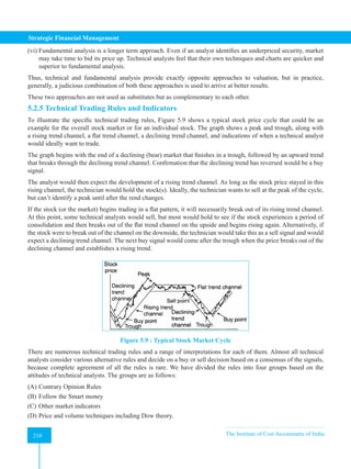
How Securitization works
Underlying assets
Reference
portfolio
(“collateral”)
Transfer of asssets from the
originator to the issuing vehicle
Assets immune from bankruptcy
of seller
Originator retains no legal interest
in assets
A
Asset originator 1
SPV issues debt securities (asset-
backed) to investors
Typically structured into various
classes/tranches, rated by one or more
rating agencies
A
Issuing agent (e.g., special
purpose vehicle [SPV])
2
Issues asset-backed
securities
Senior tranche(s)
Mezzanine
tranche(s)
Junior tranche(s)
A
Capital market
investors
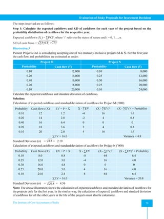
Figure 4.1: The Securitization Process
(Source: Finance & Development September 2008, IMF)
The steps can be summarized as follows:
1. The originator selects the receivables to be assigned.
2. A special purpose entity is formed.
3. The special purpose company acquires the receivables.
4. The special purpose vehicle issues securities which are publicly offered or privately placed.
5. The securities offered by the SPV are structured – usually Class A, B, C (senior, mezzanine, junior). The
ratings are driven by the size of credit support, which is, in turn, driven by the expected losses from the pool,
which are driven by the inherent risk of default in the pool.
6. The servicer for the transaction is appointed, and is normally the originator.
7. The debtors of the originator or obligors are notified depending on the legal requirements of the country
concerned. Most likely, the originator will try to avoid notification.
8. The servicer collects the receivables, usually in an escrow mechanism, and pays off the collection to the SPV.
9. The SPV passes the collections to the investors or reinvests the same to pay off the investors at stated intervals.
The pay-down to investors will follow the formula fixed in the transaction, which may either sequentially pay
Class A, B and C, or pay them proportionally, or in any other pattern.
10. In case of default, the servicer takes action against the debtors as the SPV’s agent. If losses are realized, they
are distributed in the reverse order of seniority.](https://image.slidesharecdn.com/strategyfamous-230209132502-a14bc8e7/85/Strategy_Famous-pdf-172-320.jpg)


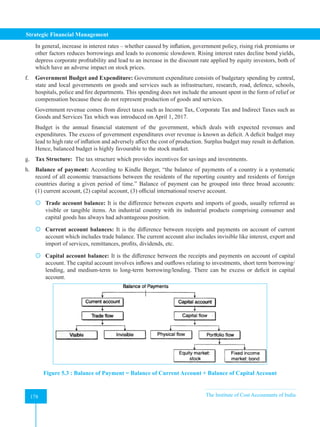
![The Institute of Cost Accountants of India 189
Introduction
(E) Growth Record:
(i) The growth in sales, net income, net capital employed and earning per share of the company in the past
few years should be examined.
(ii) The following three growth indicators may be looked into in particulars:
• Price Earnings Ratio
• Percentage Growth Rate of Earning per annum, and
• Percentage Growth Rate of Net Block
(iii) An evolution of future growth prospects of the Company should be carefully made. This requires an
analysis of:
• Existing capacities and their utilization, indicated by the quantitative information present in the
Financials,
• Proposed expansion and diversification plans and the nature of the Company’s technology, generally
indicated in the Directors’ Reports.
(iv) Growth is the most important factor in Company Analysis for the purpose of investment management. A
Company may have a good record of profits and performance in the past, but if it does not have growth
potential, its Shares cannot be rated high from the investment point of view.
(F) Financial Analysis – Intra Firm Analysis: This involves analysis of the following Ratios-
Group Ratios Considered Significance
Liquidity
Ratios
Current Ratio, Quick Ratio, Absolute Cash Ratio,
Basic Defence Interval Measure
Measure of short Term Solvency of
the Entity
Capital
Structure
Ratios
Debt to Total Funds, Equity to Total Funds, Debt –
Equity Ratio, Capital Gearing Ratio, Proprietary
Ratio, Fixed Asset to Long Term Fund Ratio
Indicative of Financing Techniques
and Long Term Solvency
Profitability
Ratios based
on Sales
Gross Profit Ratio, Operating Profit Ratio, Net Profit
Ratio, Contribution Sales Ratio [or] Profit Volume
Ratio
Indicators of the Operating and
Financial Profitability of the Entity.
Coverage
Ratios
Debt Service Coverage Ratio, Interest Coverage
Ratio, Preference Dividend Coverage Ratio
Ability to Serve Fixed Liabilities
Turnover
Ratios
Raw Material Turnover Ratio, WIP Turnover Ratio,
Finished Goods or Stock Turnover Ratio, Debtors
Turnover Ratio, Creditors Turnover ratio, Working
Capital Turnover Ratio, Fixed Assets Turnover Ratio,
Capital Turnover Ratio
They are indicative of the level of
activity and capacity utilization of
the Entity.
Overall
Return
Ratios
Return on Investment or Capital Employed, Return
on Equity (ROE) or Return on Net Worth (RONW),
Return on Assets (ROA), Earnings Per Share (EPS),
Dividend Per Share (DPS), Price Earnings Ratio (PE
Ratio), Dividend Yield (%), Book Value per Share,
Market Value to Book Value
Indicators of the Overall Profitability
and wealth Creating potential of the
Firm.](https://image.slidesharecdn.com/strategyfamous-230209132502-a14bc8e7/85/Strategy_Famous-pdf-201-320.jpg)
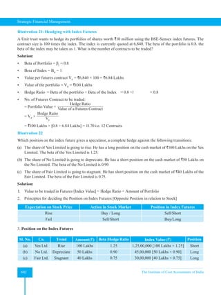
![The Institute of Cost Accountants of India 197
Introduction
It has been agreed that 4 years’ purchase of super profit shall be taken as value of goodwill for the purpose of the
deal. Value the Goodwill.
Solution:
Working Note:
i. Closing capital employed
Land and building 9,00,000
Plant and machinery 10,00,000
Trade Investments 1,00,000
Stock 2,00,000
Debtors 1,50,000
Cash 50,000
Creditors -3,00,000
Total 21,00,000
ii. Average capital employed: 21,00,000 – [(1/2) (3,00,000)] = `19,50,000
iii. Normal profit: 19,50,000 × 0.10 = `1,95,000
iv. Future maintainable profit:
Amount (`)
PBT 6,00,000
Depreciation -40,000
Additional Expenses -50,000
Tax -2,55,000
PAT 2,55,000
Super profit 2,55,000 - 1,95,000 = 60,000
Goodwill = Super Profit × No. of years of purchase = ` 60,000 × 4 = ` 2,40,000.
Illustration 2
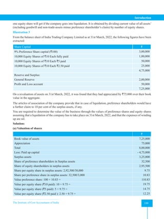
Given below is the Balance Sheet of S Ltd. as on 31st March 2022
Liabilities ` Lakhs Assets ` Lakhs
Shares Capital (10 × `10) 100 Land & Building 90
Reserve and surplus 90 Plant & Machinery 80
Creditors 30 Investments 10
Stock 20
Debtors 15
Cash & Bank 5
Total 220 Total 220
You are required to work out the value of the Company’s goodwill considering the following information:
i. Profit for the current year `64 lakhs include `4 lakhs extraordinary income and `1 lakh income from investments
of surplus funds; such surplus funds are unlikely to recur.
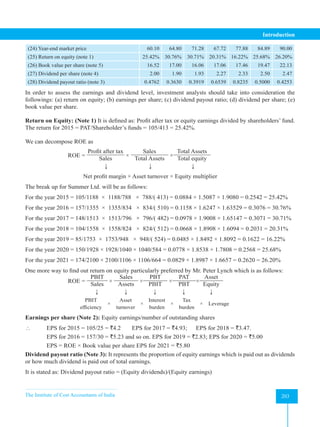
ii. In subsequent years, additional advertisement expenses of `5 lakhs are expected to be incurred each year.](https://image.slidesharecdn.com/strategyfamous-230209132502-a14bc8e7/85/Strategy_Famous-pdf-209-320.jpg)
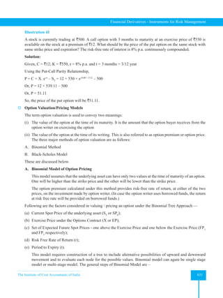
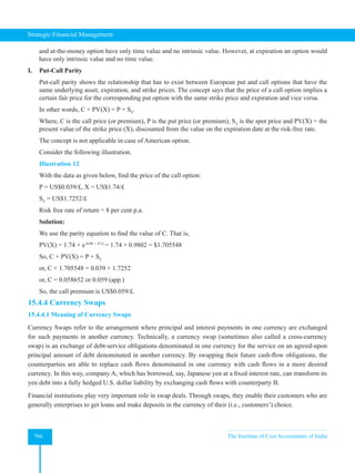
![Strategic Financial Management
202 The Institute of Cost Accountants of India
202
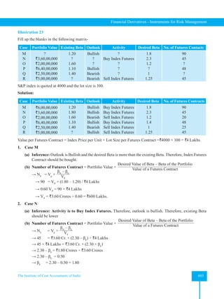
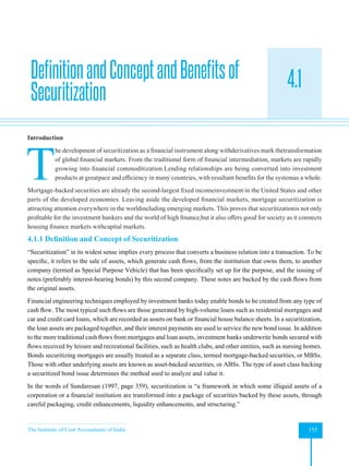
Discussion on the different angles of earnings and its effect on Company and the probable intrinsic value of
shares
When we talk about relative valuation models, we always compare price multiples of companies based on
different fundamental parameters like EPS, P/E, price-to-book value ratio, price-to-sales ratio and enterprise
value (EV/EBIT) among many. Price multiples are ratios of a stock price to some measure of value per share.
Price multiples are most frequently applied to valuation using the method of comparable. This method involves
using a price multiple to evaluate whether an asset is relatively undervalued, fairly valued or overvalued in
relation to benchmark value of the multiple. The benchmark value of the multiple may be the multiple of a
similar company or the average value of the multiple for a peer group of companies, industry, index, etc. The
economic rationale for the method of comparable is the law of one price.
No doubt, the P/E ratio is the most popular one and the key idea behind the use of P/E is that the earning power
is the chief driver of investment value and EPS is probably the primary focus which describes company’s
earnings. The P/E ratio is affected by: (a) the expected dividend payout ratio, (b) the required rate of return and
(c) the expected growth rate of dividends.
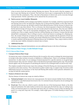
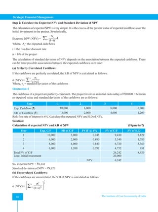
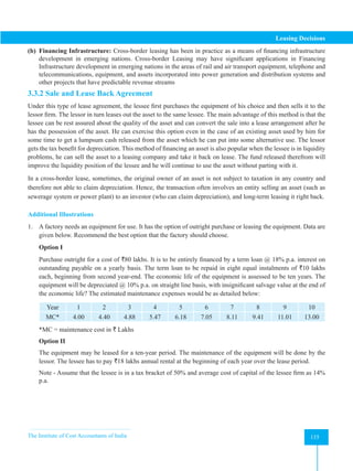
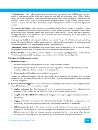
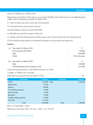
Discussion on the different angles of earnings and its effect on company and the probable intrinsic value of
the share:
Table 5.1 Financials of Summer Limited (` in lakhs)
2015 2016 2017 2018 2019 2020 2021
(1) Net sales 1188 1355 1513 1558 1753 1928 2100
(2) Cost of goods sold 880 950 1110 1188 1380 1450 1595
(3) Gross profit 308 405 403 370 373 478 505
(4) Operating expenses 88 103 110 123 150 150 185
(5) Operating profit 220 302 293 247 223 328 320
(6) Non-operating surplus/deficit 10 18 23 15 - (18) 5
(7) Profit before interest and tax (PBIT) 230 320 316 262 223 310 325
(8) Interest (I) 50 53 63 55 53 60 63
(9) Profit before tax (PBT) 180 267 253 207 107 250 262
(10) Tax (T) 75 110 105 103 85 100 88
(11) Profit after tax (PAT) 105 157 148 104 85 150 174
(12) Dividend 50 57 58 68 70 75 74
(13) Retained earnings 55 100 90 36 15 75 100
(14) Equity share capital (`10 each)(Bonus 1:5)** 250 **300 300 300 300 300 300
(15) Reserve and surplus 163 210 182 212 224 284 364
(16) Shareholders funds [14 + 15] 413 510 482 512 524 584 664
(17) Loan funds 375 324 314 312 424 456 442
(18) Capital employed [16 + 17] 788 834 796 824 948 1040 1106
(19) Net fixed assets 630 666 608 644 760 880 916
(20) Investments 45 34 32 30 30 40 50
(21) Net current assets 113 134 156 150 158 120 140
(22) Total assets 788 834 796 824 948 1040 1106
(23) Earnings per share (note 2) 4.20 5.23 4.93 3.47 2.83 5.00 5.80](https://image.slidesharecdn.com/strategyfamous-230209132502-a14bc8e7/85/Strategy_Famous-pdf-214-320.jpg)
![The Institute of Cost Accountants of India 213
Introduction
Trin =
Volume declining / Number declining
Volume advancing / Number advancing
Therefore, trin is the ratio of average volume in declining issues to average volume in advancing issues. Ratios
above 1.0 are considered bearish because the falling stocks would then have high average volume than the
advancing stocks, indicating net selling pressure. Rising volume in a rising market should not necessarily
indicate a larger imbalance of buyers versus sellers. For example, a trin statistic above 1.0, which is considered
bearish, could equally be interpreted as an indication that there is more buying activity in declining issues.
(D) Dow Theory
The oldest and best known theory of technical analysis is the Dow Theory, originally developed in 1900, by the
editor of the Wall Street Journal, Charles H Dow, who may regard as the father of technical analysis. The basic
principles of technical analysis originated from this theory. Although Dow developed the theory to describe
the past price movements. William Hamilton followed up by using it to predict movements in the market. In a
nutshell, this theory seeks to study the major movements in the market with a view to establish trends. Until a
reversal occurs, a trend is assumed to exist. It should be noted that the Dow theory only describes the direction
of market trends and does not attempt to forecast future movements or estimates either the duration or the size
of such market trends [However, subsequent analysts like Robert Rhea, who provided a formalized account of
the theory (‘The Dow Theory’), attempted to measure size and duration trends proposed by Dow].
Any discussion on technical analysis using price and volume data should begin with a consideration of the
Dow Theory because it was among the earliest work on this topic and remains the basis for many technical
indicators. (1) Major trends or primary trends are like tides in the ocean. (2) Intermediate trends that resemble
waves and (3) Short-run movements that are like ripples. Followers of the Dow Theory attempt to detect the
direction of the major price trend (tide), recognizing that intermediate movements (waves) may occasionally
move in the opposite direction. They recognize that a major market advance does not go straight up, but rather
includes small price declines as some investors decide to take profits.
Figure 5.10 : Sample Bullish Price Pattern
Figure 5.10 shows the typical bullish pattern. The technician would look for every recovery to reach a new
peak above the prior peak, and this price rise should be accompanies by heavy trading volume. Alternatively,
each profit-taking reversal that follows an increase to new peak should have a trough above the prior trough
with relatively light-trading volume during the profit-taking reversals. When this pattern of price and volume
movements changes, the major trend may be entering a period of consolidation (a flat trend) or a major reversal.](https://image.slidesharecdn.com/strategyfamous-230209132502-a14bc8e7/85/Strategy_Famous-pdf-225-320.jpg)
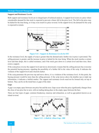
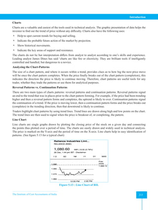
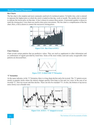
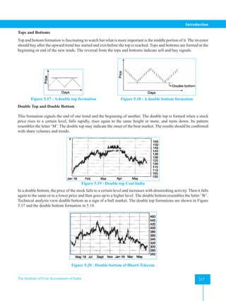
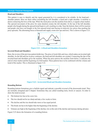
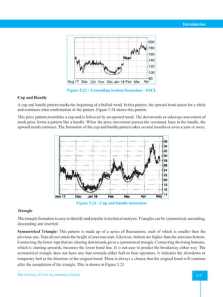
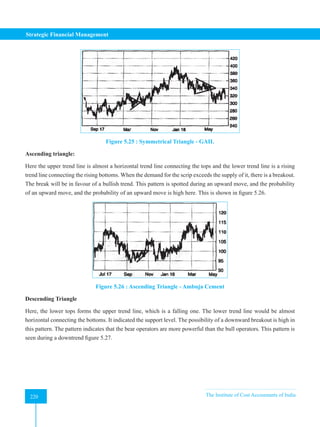
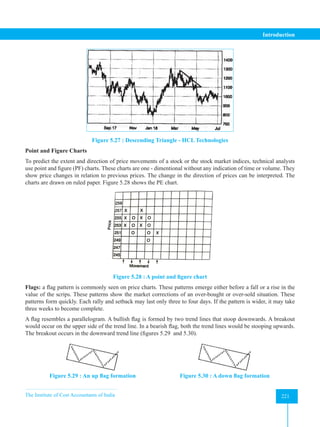
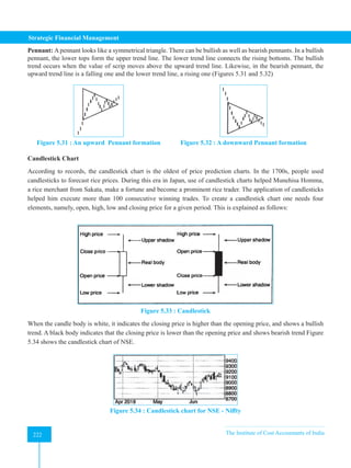
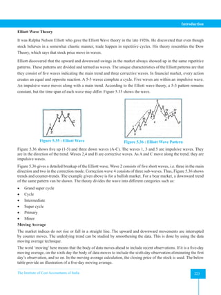
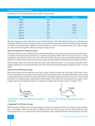
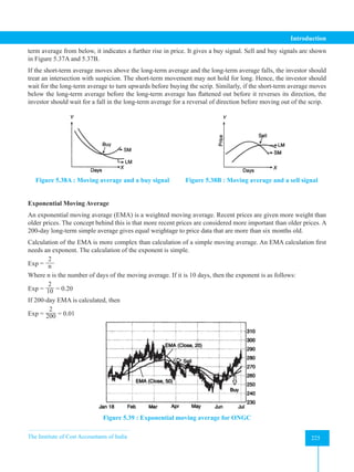
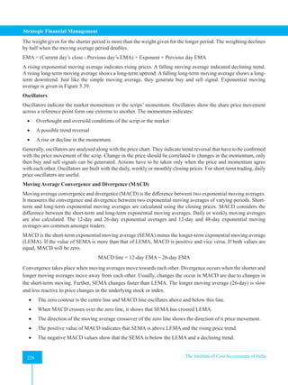
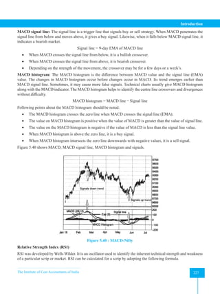
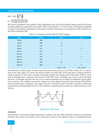
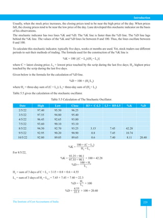
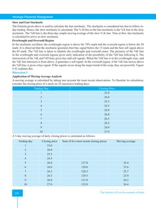
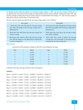
![Strategic Financial Management
232 The Institute of Cost Accountants of India
232
Solved Case Study
A financial analyst has collected the following information of MN Ltd. the details are given as follows:
(` in Million)
Particular 2018 2019 2020 2021
(a) Net sales 2,550 2,730 3,030 3,380
(b) Cost of goods sold 1,660 1,770 1,970 2,250
(c) Gross profit 890 960 1,060 1,130
(d) Operating expenses 180 200 210 250
(e) Operating profit 710 760 850 880
(f) Non-operating profit/deficit 30 40 50 -30
(g) PBIT 740 800 900 850
(h) Interest 110 130 180 200
(i) PBT 630 670 720 650
(j) Tax 190 200 220 190
(k) Profit after tax 440 470 500 460
(l) Dividend 180 190 200 160
(m) Retained earnings 260 280 300 300
(n) Equity share capital (` 10 each) 400 400 500* (Bonus 1:4) 500
(o) Reserve and surplus 400 480 500 480
(p) Shareholders’ funds [n+o] 800 880 1,000 980
(q) Loan funds 500 550 600 550
(p) + (q) = Capital employed 1,300 1,430 1,600 1,530
(r) Net fixed assets 800 880 900 860
(s) Investments 40 50 80 40
(t) Net current assets 460 500 620 630
(u) Total assets 1,300 1,430 1,600 1,530
Year end market price per share 102 107 101 107
On the basis of his information, calculate the following for the last four years:
(i) Return on equity; earnings per share; book value per share; adjusted EPS; adjusted BVPS; bonus adjustment
factor, P/E ratio (prospective); PB ratio and retention ratio.
(ii) The compounded annual growth rate of sales, CAGR EPS and volatility of ROE.
(iii) The sustainable growth rate.
(iv) Decompose the ROE in terms of five factors.
(v) Estimate the EPS for 2022 assuming an increase of 10% over the average period of last four years.
(vi) Derive the P/E ratio using the constant growth dividend model. For this purpose, assume:](https://image.slidesharecdn.com/strategyfamous-230209132502-a14bc8e7/85/Strategy_Famous-pdf-244-320.jpg)
![The Institute of Cost Accountants of India 233
Introduction
(a) dividend pay-out ratio for the average of the period of last four years.
(b) The required rate of return to be calculated based on CAPM model assuming Rf
return is 8% and market
risk premium is 26% and beta factor is 1.5.
(c) The expected growth rate in dividends is expected to be the product of the average retention ratio and the
average return on equity for the previous four years.
(vii)Find out the expected value of the stock for the year 2022 and Mr. Kapoor, a NRI would like to invest `5
million. Advise him.
Solution:
(a) Return on equity = PAT/Shareholders’ funds
(b) EPS= PAT/Number of outstanding shares
(c) Book value per share = Shareholders’ funds/Number of outstanding shares
(d) Bonus adjustment factor = Capital after bonus issue / Capital before bonus issue
Retention ratio = Retained earnings/Total equity earnings or PAT
(e) P/E ratio (prospective) = Price per share at the beginning of the year/Earnings per share for the year
(f) CAGR in sales = [sales for 2021 / sales for 2018]1/3
– 1
CAGR in EPS = [EPS for 2021 / EPS for 2018]1/3
– 1
(g) Sustainable growth rate= Retention ratio × ROE
(i)
Particular 2018 2019 2020 2021
(a) Return on Equity 0.55 0.53 0.50 0.47
(b) Book value per share (`) 20.00 22.00 20.00 19.60
(c) EPS (`) 11.00 11.75 10.00 9.20
(d) Bonus adjustment factor 1 1 1.25 1.25
(e) Adjusted EPS (`) 11.00 11.75 12.50 11.50
(f) Adjusted BVPS (`) 20.00 22.00 25.00 24.50
(g) P/E ratio (Prospective) 8.68* 10.70** 10.98***
(h) P/B ratio 5.10 4.86 5.05 5.45
(i) Retention ratio 0.59 0.60 0.60 0.65
*102/11.75; **107/10.00; ***101/9.20.
(ii) CAGR in Sales = (3380/2550)1/3
– 1 = (1.3255)1/3
– 1 = 9.85%
CAGR in EPS = (11.50/11.00)1/3
– 1 = (1.0455)1/3
– 1 = 1.49%
Volatility of return on equity = 55-47/51.25 = 15.61%
(iii) Sustainable growth rate = [(0.59+0.60+0.60+0.65)/4] [(55+53+50+47)/4]
= 0.61 × 51.25 = 31.26%](https://image.slidesharecdn.com/strategyfamous-230209132502-a14bc8e7/85/Strategy_Famous-pdf-245-320.jpg)
![Strategic Financial Management
234 The Institute of Cost Accountants of India
234
(iv) ROE = (PBIT/Sales) × (Sales/Assets) × (PBT/PBIT) × (PAT/PBT) × (Asset/Equity)
For 2018 = (740/2550) × (2550/1300) × (630/740) × (440/630) × (1300/800)
= 0.2902 × 1.9615 × 0.8514 × 0.6984 × 1.625= 0.55.
For 2019 = 0.53
For 2020 = 0.50 [Average = (0.55+0.53+0.50+0.47)/4 = 0.5125]
For 2021 = 0.47
(v) Average adjusted EPS = [(11.00 + 11.75 + 12.50 +11.50)/4] = 46.75/4 = 11.69
Expected EPS for 2022 = 11.69 × 1.10 = ` 12.86
(vi) Average retention ratio for the period 2018 to 2021 = 0.61[(0.59+0.60+0.60+0.65)/4]
So, the average dividend pay-out ratio was (1 -0.61) or 0.39
Required rate of return as per CAPM = Rƒ
+β (Rm
- Rƒ
) = 8 + (26 - 8) × 1.5 = 35%.
g = average ROE × average retention ratio
Expected growth rate in dividends = 51.25 × 0.61 = 31.26%
P/E ratio as per the constant growth model = D1
/r – g = 0.39/(0.35-0.3126) = 10.43
The value per share = Expected P/E ratio × EPS = 10.43 × 12.86 or ` 134
As the intrinsic value is much higher it is better to invest in stocks of MN Ltd.](https://image.slidesharecdn.com/strategyfamous-230209132502-a14bc8e7/85/Strategy_Famous-pdf-246-320.jpg)
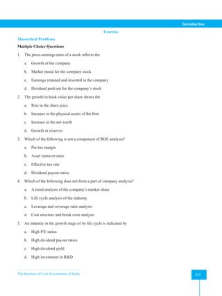
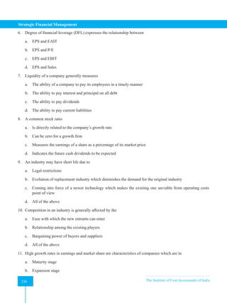
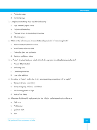
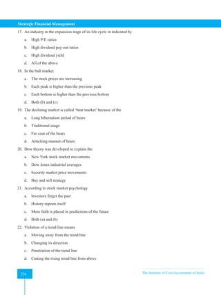


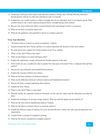
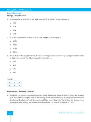
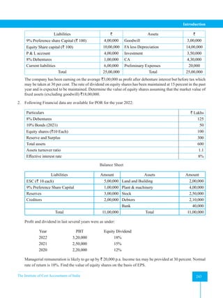
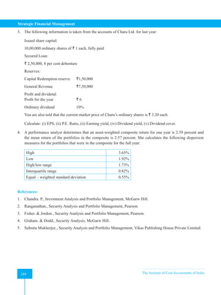
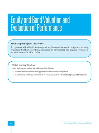
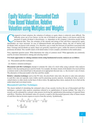
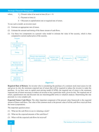
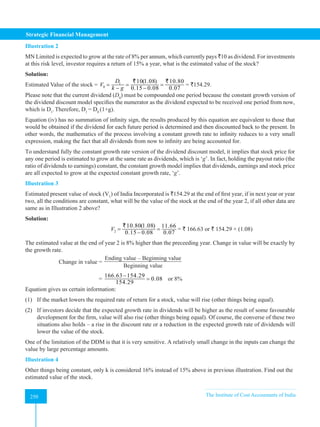
![The Institute of Cost Accountants of India 251
Equity and Bond Valuation and Evaluation of Performance
Solution:
Estimated value at the end of year 0(1 ) 10(1.08)
1
0.16 0.08
D g
k g
+
= =
− −
`
= ` 135
Conclusion: One percentage change in required return causes [(154.29 – 135)/154.29] or 12.5% change in value
(decrease).
Illustration 5
Other things being constant as in Illustration 4, growth rate is considered 9% instead of 8%, find out the new
valuation of stock.
Solution:
The new valuation of stock =
10(1.09) 10.90
0.15 0.09 0.06
=
−
= ` 181.67
An increase of previous value by 17.74%. Only one percent change in growth rate amounts to 17.74% change
in price of the stock. Last assumption, required rate of return increased from 15% to 18% and the growth rate has
dropped from 8% to 4%.
The new price of the stock will be: 10(1.04) 10.04
0.18 0.04 0.14
=
−
` `
` 10.4
= ` 74.29
Therefore, the estimated value declines by 51.85% compared with the original value `154.29 (Illustration 2).
These differences suggest why stock prices constantly fluctuate as investors make their buy and sell decisions.
Even if it is assumed that all investors will follow DDM, still there will be differences in estimation of value of
the stock because:
(a) Each investor has his or her own required rate of return, resulting wide variety of ‘k’.
(b) Each investors have their own growth rate expectations in dividends. Small differences in growth rate (g)
produces significant differences in price, everything else held.
Thus, at any point in time for a particular stock, some investors are willing to buy, whereas others wish to sell,
depending on their estimate of the intrinsic value of the stock. This helps to make market active and liquid.
Equation (iv) can be modified to include the earnings per share. Assuming a constant pay-out ratio, it can be
rewritten as:
1 1
(1 )
b E D
V
k g k g
−
= =
− −
[where b is the retention rate] ... ... ... (v)
Estimating the Capitalization Rate
The capitalization rate can be determined from the constant growth of dividend capitalization model. Under this
approach, the required rate of return on the equity capitalization rate (k) will be as follows:
1
0
D
k g
P
= +
... ... ... (vi)
where P0
= present value of the stock, k = capitalization rate, D1
= dividend one year hence and g = growth rate.](https://image.slidesharecdn.com/strategyfamous-230209132502-a14bc8e7/85/Strategy_Famous-pdf-263-320.jpg)
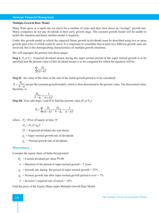
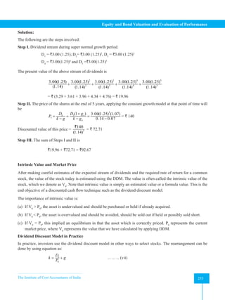
![Strategic Financial Management
254 The Institute of Cost Accountants of India
254
This equation states that the expected rate of return on a constant growth stock, ‘k’ is the dividend yield plus the
expected growth in dividends and price ‘g’. The latter term may be considered as the price change component or
capital gains component. Therefore, an investor’s expected rate of return from a stock is the sum of the income
component and the price change component which together constitute the total return from a stock.
Illustration 7
A company’s share is currently traded for `80 per share. It is expected that a dividend of `4 per share after one year
will grow at 8% indefinitely. What is the expected return?
Solution:
k = [(Div1
)/P0
] + g = [4/80] + 0.08 = 0.13 or 13%
Three-Phase Model
Here, three phases of dividend growth pattern is assumed. Dividends are assumed to grow at a constant rate ‘g’ for
a period of ‘A’ years. After the phase ‘A’, the growth rate of dividend declines for A + 1 years throughout phase
B and the decline in the dividend rate would be linear. Afterwards, there would be perpetual growth rate ‘gn
’.
Sometimes the ‘ga
’would be less than ‘gn
’ and in the second phase there would be linear growth rate. The perpetual
growth rate is known as the firm’s long-run normal growth rate. Figure illustrates the three-stage growth rates.
ga
Phase I
Phase II
Phase III
Time
gb
Figure 6.2: Three-phase model of stock return and valuation
0 1
0
1 1
(1 ) (1 ) (1 )
(1 ) (1 ) (1 )
A B
t
a t b B n
t t B
n
t t A
D g D g D g
P
k k k g k
−
= = +
+ + +
= + +
+ + − +
∑ ∑
where D0
= Next year dividend
ga
= Period ‘A’ growth rate (Phase I)
gb
= Period ‘B’ growth rate (Phase II)
gn
= Growth rate in the third phase
DB
= Dividend at the beginning of the third phase
Illustration 8
For the first four years, India Incorporated is assumed to grow at a rate of 10%. After four years, the growth rate of
dividend is assumed to decline linearly to 6 percent. After 7 years, it is assumed to grow at a rate of 6% infinitely.
The next year dividend is `2.00 per share and the required rate of return is 14%. Find the value of the stock.](https://image.slidesharecdn.com/strategyfamous-230209132502-a14bc8e7/85/Strategy_Famous-pdf-266-320.jpg)
![Strategic Financial Management
256 The Institute of Cost Accountants of India
256
multiple of 20. In another stock, if the earnings per share is `5.00 and is selling at the same price of `200, it is said
that the share is selling at a multiple of 40. It denotes that the market price of the share is 40 times the earnings per
share. P/E ratio is published by the financial press on a regular basis.
It is by definition that
P0
= Current stock price = E0
× P0
/E0
where, P0
= current stock price and E0
= the most recent 12 month earnings per share.
It is worth nothing that stock price is the product of two variables when using this type of approach.
(1) EPS and (2) P/E multiple. (EPS states earnings per share).
Determinants of P/E ratio: The P/E ratio can be derived from the dividend discount model which is the foundation
of valuation for common stocks. Please note that this process directly applies only for the case of constant growth. If
a multiple growth model is applicable to the stock being considered, a different formulation from the one presented
here will be needed. In fact, using the P/E ratio for multiple growth rate companies can be misleading and should
be done with care.
Consider equation (iv) using the constant growth version of the model. The value of a stock or
1
D
P
k g
=
−
[recall Equation (v)]
Dividing both sides of the equation by expected earnings E1
1 1
1
/
/
D E
P E
k g
=
−
... ... ... (viii)
Equation (viii) indicates those factors that affect the estimated P/E ratio.
If the growth rate is assumed to depend on the return on equity (ROE), then g = ROE (1 – d1
/e1
)
Then, 1
0
d
P
k g
=
−
can be written as 1 1
1 1
1 1
/
/
(1 / )
d e
P E
k ROE d e
=
− −
Thus, P/E ratio depends on the dividend payout, discount rate and return on equity and all these factors affect
the P/E multiple.
Variables that impact on growth of price, return and P/E ratio.
1. The expected dividend payout ratio, D1
/E1.
2. The required rate of return which has to be estimated.
3. The expected growth rate of dividends.
The following relationship should hold, other things being equal:
1. The higher the expected payout ratio, the higher the P/E ratio.
2. The higher the expected growth rate (g), the higher the P/E ratio.
3. The higher the required rate of return (k), the lower the P/E ratio.](https://image.slidesharecdn.com/strategyfamous-230209132502-a14bc8e7/85/Strategy_Famous-pdf-268-320.jpg)
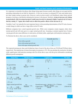
![Strategic Financial Management
258 The Institute of Cost Accountants of India
258
Looking at the table, we can come into the conclusion that:
1. Other things being equal, as the expected growth in dividends increases the expected return, i.e. total return
(= dividend yield + capital gain) depends more on the capital gain less on the dividend yield.
2. Other things being equal, the price-earnings ratio increases as the expected growth rate in dividend increases.
3. High dividend yield and low price-earnings ratio imply limited growth prospects.
4. Low dividend yield and high price-earnings ratio imply considerable growth prospects.
Understanding the P/E Ratio
Most investors intuitively realize that the P/E ratio should be higher for companies whose earnings are expected
to grow rapidly. However, how much higher is not an easy question to answer. The market will assess the degree
of risk involved in the expected future growth of earnings – if the higher growth rate carries a high level of risk,
the P/E ratio will be affected accordingly. Future more, high growth rate may be attributable to several different
factors, some of which are more desirable than others.
P/E ratio reflects investors expectations about the growth potential of a stock and the risk involved. These two
factors can offset each other. Other things being equal, the greater the risk of a stock, the lower the P/E ratio;
however, growth prospect may offset the risk and lead to a higher P/E ratio. The internet companies that were so
popular in the late 1990s were clearly very risky but investors valued their potential very highly and were willing
to pay very high prices for these companies.
The required rate of return, in turn, is also closely related to interest rates, which are the required returns on bonds.
As interest rates increase, required rate of return on all securities, including stock, also generally increase. As
interest rates increase, bonds become more attractive compared to stocks on a current return basis. There is an
inverse relationship between P/E ratios and interest rates. As interest rates rise (decline), other things being
equal, P/E ratios should decline (rise).
Price-earnings is derived: g = b × ROE, P0
= D1
/(k – g) or P0
/E1
= (1 – b)/[k – (ROE × b)].
The growth rate of a growing firm that is sustainable equals to P0
/E1
.](https://image.slidesharecdn.com/strategyfamous-230209132502-a14bc8e7/85/Strategy_Famous-pdf-270-320.jpg)
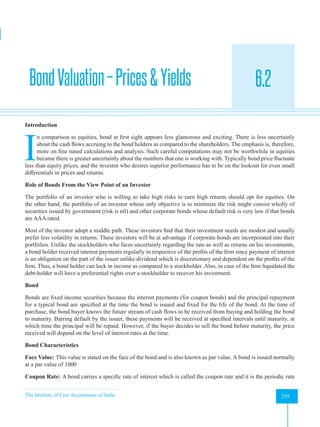
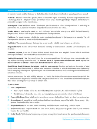
![The Institute of Cost Accountants of India 261
Equity and Bond Valuation and Evaluation of Performance
become due on specified dates prior to maturity. They are termed as serial bonds.
Puttable Bonds: A puttable bond grants the bondholder the right to sell the issue back to the issuer at par value
on designated dates.
Callable Bonds: These bonds refer to the ability of the issuer to pay off a debt obligation prior to its maturity
at the option of the issuer of debt.
Exchangeable Bonds: It grants the bondholder the right to exchange the bonds for the common stock of a firm
other than that of the issuer of the bond.
Fixed Rate Bonds: These are bonds with a coupon or a stated rate of interest which remains constant throughout
the life of the bond.
High Yield Bonds: They are bonds that are rated below investment grade by the credit rating agencies. They
are also called junk bonds.
Mortgage Bonds: A bond that is secured through a lien against the property of the firm is known as mortgage
bond.
Subordinated Bonds: These bonds have a lower priority than secured debts, debentures and other bonds and
the general creditors of the issuer in case of liquidation.
Guaranteed Bonds: It is an obligation guaranteed by another entity.
Perpetual Bonds: These bonds are also called perpetuities. It has no maturity date.
Global bonds: Bonds that are designed so as to qualify for immediate trading in any domestic capital market
and in the Euro market are called global bonds.
Easy Exit Bonds: These are bonds which provide easy liquidity and exit route to investors by way of
redemption or buy back facility where investors can get the benefit of ready encashment in case of need to
withdraw before maturity.
Option Bonds: These are cumulative and non-cumulative bonds where interest is payable on maturity or
periodically. Redemption premium is also offered to attract investors. These were issued by institutions like
IDBI, ICICI, etc.
Double Option Bonds: The face value of each bond is `5,000. The bond carries interest at 15% p.a.
compounded half-yearly from the date of allotment. The bond has a maturity period of 10 years. Each bond has
two parts in the form of two separate certificates, one for principal of `5,000 and other for interest (including
redemption premium) of `16,500. Both these certificates are listed on all major stock exchanges. The Investor
has the facility of selling either one or both parts at anytime he wishes so.
Floating Rate Bonds: Here, Interest rate is not fixed and is allowed to float depending upon the market
conditions. This is an instrument used by the issuing Companies to hedge themselves against the volatility in
the interest rates. Financial institutions like IDBI, ICICI, etc. have raised funds from these bonds.
Inflation Bonds: Inflation Bonds are bonds in which interest rate is adjusted for inflation. Thus, the investor
gets an interest free from the effects of inflation. For example, if the interest rate is 10% and the inflation is 2%,
the investor will earn 12.20% [i.e. (1 + Interest Rate) × (1 + Inflation Rate) -1]. This is similar to Floating Rate
Bonds, i.e. rate of return varies over a period of time.](https://image.slidesharecdn.com/strategyfamous-230209132502-a14bc8e7/85/Strategy_Famous-pdf-273-320.jpg)
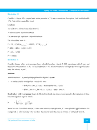
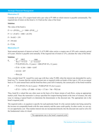
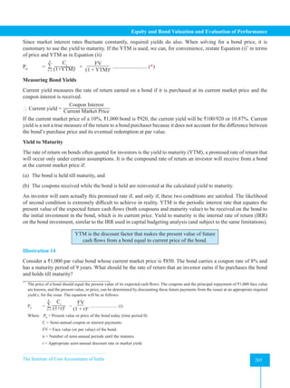
![Strategic Financial Management
266 The Institute of Cost Accountants of India
266
Solution:
P = ∑
Ct
(1+YTM)t
n
t=1
+
FV
(1 + YTM)n
We know Ct
= ₹80 annual, FV = ₹1,000, n = 9 years, YTM = ?
Through financial calculator or computer excel spreadsheet, we can easily find out YTM = 10.67% for annual and
10.63% semi-annual.
A B C
Settlement date 01-01-2013 01-01-2013
Maturity date 01-01-2022 01-01-2022
Annual coupon rate 0.08 0.08
Bond price (Flat) 85 85
Redemption value 100 100
Coupon payment per year 2 1
Yield to maturity 0.1063 0.1067
Semi-annual coupons Annual coupons
Formula used
B9 =YIELD (B2,B3,B4,B5,B6,B7)
C9 =YIELD (C2,C3,C4,C5,C6,C7)
The yield to maturity calculation for zero coupon bond is here on the same process expressed in the above equation,
equating the current price to the future cash flow to find YTM, and then doubling the result to obtain the annual
YTM, because there are no coupons, the only cash flow is the face value of the bond to be received at maturity. The
YTM calculation for a zero coupon bond will be as follows:
YTM = [FV/P]1/n
- 1
An approximation: Instead of trial and error, we have an another method to find the approximate YTM on a bond:
YTM =
C + (M - P)/n
0.4 M + 0.6 P
where YTM is the yield to maturity, C is the annual coupon payment, M is the maturity value of the bond, P is the
present value of the bond, n is the years to maturity. Consider Illustration 22:
YTM =
80 + (1000 - 850)/9
0.4 × 1000 + 0.6 × 850
=
80 + 16.66
400 + 510 = 10.62%
Yield to Call: Most corporate bonds, as well as government bonds, are callable by the issuers, typically after some
deferred call periods. For bonds likely to be called, the yield to maturity calculation is unrealistic and a better
calculation is the yield to call.](https://image.slidesharecdn.com/strategyfamous-230209132502-a14bc8e7/85/Strategy_Famous-pdf-278-320.jpg)
![The Institute of Cost Accountants of India 267
Equity and Bond Valuation and Evaluation of Performance
Illustration 15
Suppose the 8% coupon, 20-year maturity bond sells for ₹1,120 and is callable in 10 years at a call price of ₹1,090.
Calculate its yield to maturity and yield to call using the following inputs:
Yield to call (₹) Yield to Maturity (₹)
Coupon Payment 40 40
Number of Semi-annual periods 20 40
Final payment 1,090 1,000
Present Price 1,120 1,120
Solution:
With the help of spreadsheet, we can easily calculate: Yield to call = 6.95% or yield (issue date as 01- 01- 2003,
01-01-2013, interest .08% present price 112, redemption price 109, no. of installments in a year 2). Yield to maturity
= 7.00%
A B
Semi-annual coupons
Settlement date 1-1-2012
Maturity date 1-1-2022
Annual coupon rate 0.08
Bond Price (flat) 112
Redemption value 109
No. of installments in a year 2
Yield to call 0.0695
Formula uses
B9 yield to call = Yield (B2, B3, B4, B5, B6, B7)
Realized Compound Yield
After the investment period for a bond is over, an investor can calculate the Realized Compound Yield (RCY).
This rate measures the compound yield on the bond investment actually earned over the investment period, taking
into account all immediate cash flows and reinvestment rates. The semi-annual realized compound yield can be
calculated using the following formula:
RCY =
Total ending wealth
Purchase Price of bond
[ ]
1/n
-10
Assume an investor had ₹1,000 to invest 2 years ago. This investor purchased a 10% coupon bond with a two-year
maturity at face value. The promised YTM for this bond was 10%. Assume that investor invested exactly at 10%
at the end of each year and after 2 years the amount would come exactly at ₹ 1,210.](https://image.slidesharecdn.com/strategyfamous-230209132502-a14bc8e7/85/Strategy_Famous-pdf-279-320.jpg)
![Strategic Financial Management
268 The Institute of Cost Accountants of India
268
At time (0) - the amount of investment = ₹1,000
Add: Interest at the end of 1st year re-invested @10% = ₹ 100
Opening balance at the beginning of year 2 = ₹1,100
Add: Interest at the end of 2nd year re-invested @10% = ₹ 110
Ending value ₹1,210
P2
= P0
[(1 + r)2
]
Or, ₹1,000 (1 + r)2
= ₹1,000 [(1 + 0.10)2
] = ₹1,210 or r = 0.10 = 10%
With a reinvestment rate equal to the 10% yield to maturity, the realized compound return equals to yield to
maturity.
Price Yield Relationship
The earlier section discussed price of bond. However, it is required to understand different types of bond yield. The
commonly employed bond yield measures are:
(i) Current yield: The current yield relates the annual coupon interest to the market price. It is calculated by using
the formula:
Current Yield = Annual Interest/Price
(ii) Yield to Maturity: The yield to maturity (YTM) is defined as the interest rate that makes the present value of
a bond’s payments equal to its price. This interest rate is often interpreted as a measure of the average rate of
return that will be earned on a bond if it is bought now and held until maturity.
(iii) Yield to Call: Some bonds carry a call feature that entitles the issuer to call (buy back) the bond prior to the
stated maturity date in accordance with a call schedule.
The basic property of a bond is that its price varies inversely with yield. If the required yield decreases, the present
value of the cash flow increases; hence the price of the bond increases. Conversely, when the required yield
increases, the present value of cash flow decreases. The higher the coupon rate, the smaller the percentage price
change due to any given change in interest rate are positively related. The graph of the price-yield relationship for
the bond has a convex shape.
The relationship between the coupon rate, the required yield and the price of bond is as follows:
Coupon Rate > Required Yield Price > Par (Premium Bond)
Coupon Rate = Required Yield Price = Par
Coupon Rate < Required Yield Price < Par (Discount Bond)
Consider, a bond carrying a coupon rate of 14% issued 3 years ago for `1,000 (its par value) by XYZ Co. The
original maturity of bond was 10 years, so its residual maturity now is 7 years. The interest rate is fallen in the last
3 years and investors now expect a return of 10% from this bond. So the price of the bond now would be `1,194.70
(based on the formula mentioned above).](https://image.slidesharecdn.com/strategyfamous-230209132502-a14bc8e7/85/Strategy_Famous-pdf-280-320.jpg)
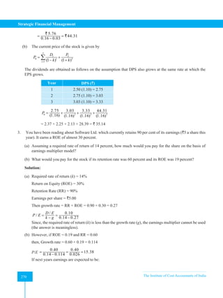
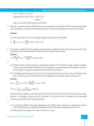
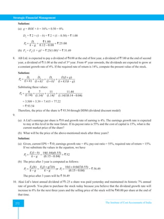
![Strategic Financial Management
274 The Institute of Cost Accountants of India
274
Solution
Through excel presentation yield to maturity = 14.68% or
YTM = [1+(F-P)/n ]/[0.4F+ 0.6 P] = 60 +[(995-700)/5]/[0.4 (995)+0.6(700)] = (60 +59)/(398+420) = 119/818
= 14.54%
14. A financial institution issues two types of bonds with one year and another three years’ maturity respectively.
The first, which pays `10,000 a year hence, is now selling for `8,929. The second which pays `100 next years,
`100 after two years and `1,100 at the end of third year is now offered at `997.18. Find out the implied rates
of these two bonds.
Solution:
Assume k1
and k2
are the implied interest rates on bonds I and II, respectively.
Bond I:
` 10,000 PVIF(k₁, I) = ` 8929
or `10,000 / (1+k₁) = ` 8929 or ` 8929 (1+k₁) = ` 10,000
or Solving, we get k1
, = 12%
Bond II:
977.18 = 100 PVIF (k₂, I₁) + 100 PVIF (k2
, I2
) + ` 1100 PVIF (k₂, I3
)
or 977.18 = 100/(1+k2
) + 100/(1+k2
)2
+ 1100/(1+k2
)3
Solving, we get k₂ = 10.1%
Implied interest rate on bond, I and II are, respectively, 12% and 10.1%.
15. An AAA rated bond of face value `1,000 is currently quoting in the market at `1,062. The coupon rate of
the bond is 14% payable semi-annually. The remaining maturity of the bond is five years and the principal is
repayable at two equal instalments at the end of the 4th and 5th year form now. Find out the YTM of the bond.
Solution:
The required YTM is given by r in the following equation:
1062 = 70 PVIFAr,8
+ 500 × PVIFr,8
+35 PVIFr,9
+ 535 × PVIFr,10
for r = 6%,
RHS = 70 × (6.210) + 500 × (0.627) + 35 × (0.592) + 535 × 0.558 = `1067.45
for r = 7%,
RHS = 70x (5.971) + 500 × (0.582) + 35 × (0.544) + 535 × (0.508) = ` 999.79
r = 6%+(7-6) % × (1067.45-1062)/(1067.45-999.79) = [(6+1)×5.45]/67.66 = 6.08%
Required rate = 6.08 × 2 = 12.16%
16. A company is offering a bond with the issue price of ` 100, annual coupon rate is 12% with maturity period 5
years. If the bond is to be redeemed at par and the investor faces a 30% tax on income and a 10% capital gains
tax, find out the effective yield to maturity for the investor.](https://image.slidesharecdn.com/strategyfamous-230209132502-a14bc8e7/85/Strategy_Famous-pdf-286-320.jpg)
![The Institute of Cost Accountants of India 275
Equity and Bond Valuation and Evaluation of Performance
Solution:
Let the yield to maturity be ‘i’, then,
100 = 12 × 0.7 × PVIFA(i,5)
+ 100 PVIF(i, 5)
Solving, we get i = 8.41%
17. A Ltd. issued bonds face value ` 1,000 having a maturity premium of 10% and a coupon rate of 9%. The
bonds are presently trading at par. The yield to maturity of the bond to an investor as of now, by approximation
method, is 12%. What will be the approximate maturity period for the bonds?
Solution:
Let the approximate maturity period be n years and the face value of the bond be ` 1,000.
YTM through approximation method would be
YTM = 1+ [(F-P)/n] /[(F+P)/2]
We have I = ` 90; P = ` 1000; F = ` 1100 and YTM = 12%
0.12 = 90+[(1100-1000)/n]/[(1100 +1000)/2]
or 0.12 = [(90+100)/n]/1050
or n=2.78 years
18. Two bonds have identical times to maturity and coupon rates. One is callable at `105, the other at `110. Which
should have the higher yield to maturity? Why?
Solution:
The bond callable at `105 should sell at a lower price because the call provision is more valuable to the firm.
Therefore, its yield to maturity should be higher.
19. Which security has a higher effective annual interest rate?
(a) A 3-month T-bill selling at ` 97,645 with par value ` 1,00,000.
(b) A coupon bond selling at par and paying a 10% coupon semi-annually
Solution:
(a) Effective annual rate for 3-month T-bill;
(1,00,000/97,645)4
– 1 = 10%
(b) Effective annual interest rate for coupon bond paying 5% semi-annually:
(1.052
-1) = 0.1025 or 10.25%.
Therefore, the coupon bond has the higher effective annual interest rate.
20. Consider a bond with 10% coupon and with YTM = 8%. If the bond’s YTM remains constant, then in 1 year,
will the bond price be higher, lower or unchanged? Why?
Solution:
The bond price will be lower. As time passes, the bond price, which is now above par value, will approach par.](https://image.slidesharecdn.com/strategyfamous-230209132502-a14bc8e7/85/Strategy_Famous-pdf-287-320.jpg)
![The Institute of Cost Accountants of India 277
Equity and Bond Valuation and Evaluation of Performance
NPV at 18% = -190 + (1000 × 0.191) = + 1
As NPV (at 18%) is positive, this shows that the return is greater than 18%.
Let’s calculate NPV at 19%.
NPV at 19% = -190+ (1000 × 0.176) = - 14
As NPV (at 19%) is negative, this shows that the return is less than 19%.
We can find the exact return (called YTM, also called current interest rate) through interpolation.
YTM or current interest rate:
= Lower rate +
Lower rate NPV
(Lower rate NPV - Higher rate NPV)
× (difference in rates)
= 18 +
1
1 - (-14)
× 1 = 18.066%.
Solved Case Study
Naveen has joined Excel Corporation as a finance trainee. He has given the following details and have been
asked to find out the following which are as follows:
The current yield curve for default free zero coupon bonds is as follows:
Maturity (years) YTM %
1 10
2 11
3 12
(a) What are the implied 1-year forward rates?
(b) Assume that the pure expectations hypothesis of the term structure is correct. If the market expectations
are accurate, what will be the pure yield curve (that is, the yields to maturity on 1-year and 2-year zero
coupon bonds) next year?
(c) If an investor purchase a 2-year zero coupon bond now, what is the expected total rate of return over the
next year? What if you purchase a 3-year zero coupon bond? Ignore taxes.
(d) What should be the current price of a 3-year maturity bond with a 12% coupon rate paid annually? If you
purchased it at the price, what would be your total expected rate of return over the next year (coupon plus
price change)? (Ignore taxes).
Solution:
(a) We obtain forward ate from the following table:
Maturity YTM Forward Rate Price [for parts (c) and (d)]
1 year 10% --- ₹1000/1.10 = ₹909.09
2 years 11% (1.112
/ 1.10) – 1 =12.01% ₹1000/1.112
= ₹811.62
3 years 12% (1.123
/ 1.112
) – 1 = 14.03% ₹1000/1.123
= ₹711.78](https://image.slidesharecdn.com/strategyfamous-230209132502-a14bc8e7/85/Strategy_Famous-pdf-289-320.jpg)
![Strategic Financial Management
278 The Institute of Cost Accountants of India
278
(b) We obtain next year’s prices and yields by discounting each zero’s face value at the forward rates for next
year that we derived in part (a).
Maturity Price YTM
1 year ₹1000/1.1201 = ₹892.78 12.01%
2 years ₹1000 / (1.1201 × 1.1403) = ₹782.93 13.02%
Please note that this year’s upward sloping yield curve implies, according to the expectation hypothesis, a
shift upward in the next year’s curve.
(c) Next year, the 2-year zero will be a 1-year zero, and will therefore sell at a price of: ₹1000/1.1201
= ₹892.78. Similarly, the current 3-year zero will be a 2-year zero and will sell for ₹782.93.
Expected total rate of return:
2-year bond = (₹892.78 ÷ ₹811.62) - 1 = 1.1000 – 1 = 10%
3-year bond = (₹782.93 ÷ ₹711.78) - 1 = 1.1000 – 1 = 10%
(d) The current price of the bond should equal to the value of each payment times the present value of ₹1 to
be received at the “maturity” of that payment. The present value schedule can be taken directly from the
prices of zero-coupon bonds calculated above.
Current price = (₹120 × 0.9090) + (₹120 × 0.8116) + (₹1,120 × 0.71178) = ₹1,003.68
Similarly, the expected prices of zeros one year from now can be used to calculate the expected bond value
at that time.
Expected price 1 year from now = (₹120 × 0.89278) + (₹1,120 × 0.78293) = ₹984.02
Total expected rate of return = [₹120 + ₹(984.02 - 1003.68) ÷ 1003.68] = 10%](https://image.slidesharecdn.com/strategyfamous-230209132502-a14bc8e7/85/Strategy_Famous-pdf-290-320.jpg)

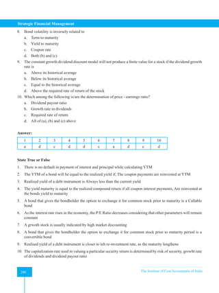
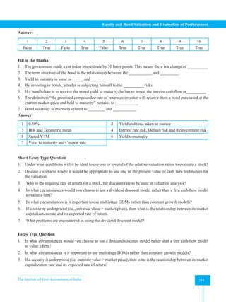
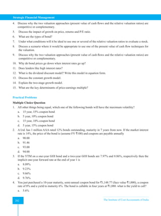
![The Institute of Cost Accountants of India 283
Equity and Bond Valuation and Evaluation of Performance
b. 6.0%
c. 7.2%
d. 8.0%
[Hints: n = 8; call price = `1080; semi-annual interest payment will be `40. spreadsheet or calculator entries
will be N = 8; PV = -1148.77; PMT = 40, FV = 1080, CPT 1/Y 2.80. the annual yield to call = 2.80 × 2 = 5.60%]
5. A 20-year maturity bond with a par value `1,000 makes semi-annual payments at a coupon rate of 8%. The
YTM is 9%. How much should you pay for the bond?
a. `1080
b. `1000
c. `908
d. `966
6. A bond with a par value of `1,000 has a 6% annual coupon rate. Interest is paid semi-annually and the price of
the bond is `1,025. what is the current yield?
a. 3.0%
b. 2.9%
c. 6.2%
d. 5.9%
7. A semi-annual coupon bond is currently selling for `1,142.12. The bond has a maturity of 10 years, a par value
of `1,000 and a 9% coupon rate. What is the yield to maturity?
a. 3.5%
b. 7.0%
c. 7.5%
d. 9.0%
8. One year ago, you purchased an annual coupon bond for `817.84. At that time the bond had a maturity of 15
years, a face value of `1,000, a coupon rate of 5% and a yield to maturity of 7%. One year later, the yield to
maturity increased to 7.5%. what is the total rate of return for the year?
a. 9.79%
b. 2.44%
c. 7.50%
d. 3.75%
9. Mr. X expects 20% return from his investment. The dividend from the stock is `2.0 and the present price is
`50. What should be the future price of the stock?
(a) ` 56.39
(b) ` 58.00
(c) ` 60.00
(d) ` 62.30
10. A stock of `10 face value has declared 35% dividend for the current year. The stock is currently selling for `40.
What I the dividedly yield?
(a) 35%
(b) 8.75%](https://image.slidesharecdn.com/strategyfamous-230209132502-a14bc8e7/85/Strategy_Famous-pdf-295-320.jpg)
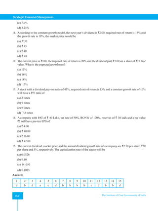
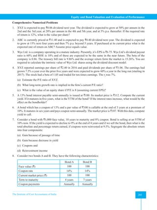
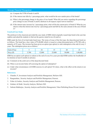

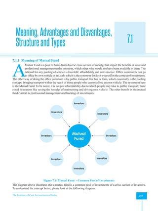
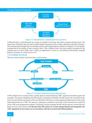
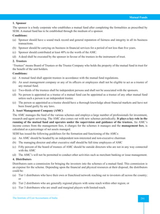
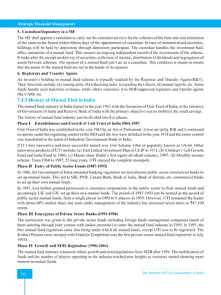
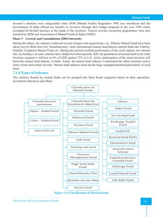
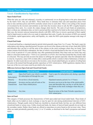
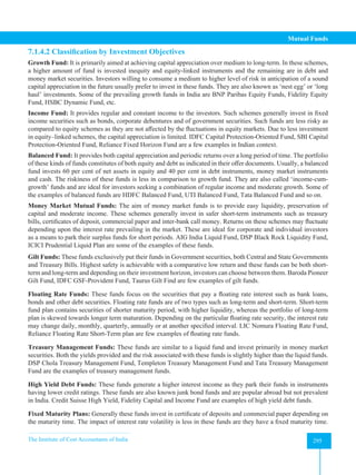
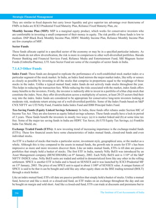
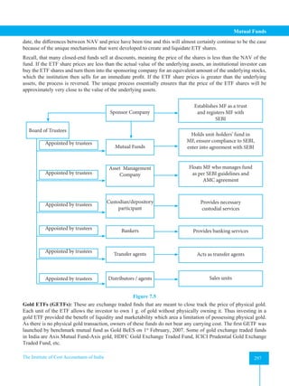
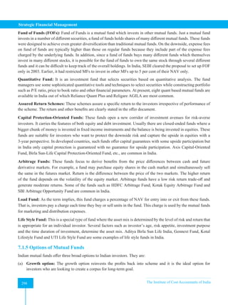
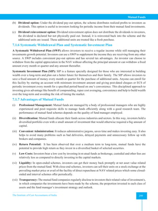
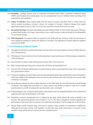
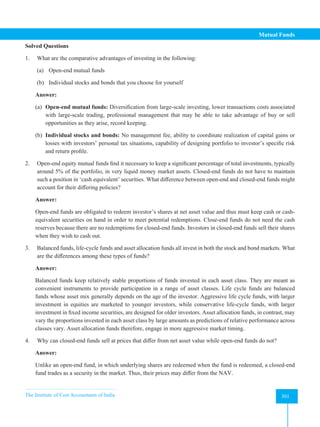
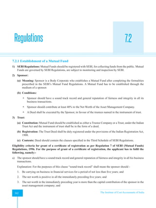
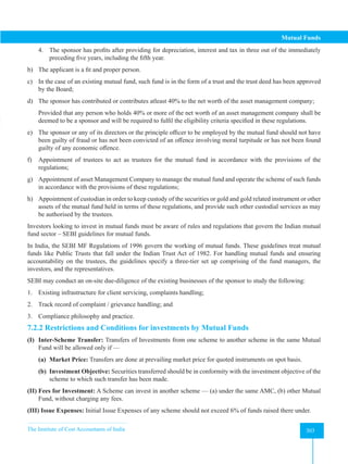
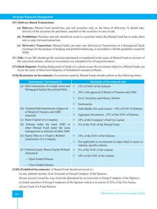
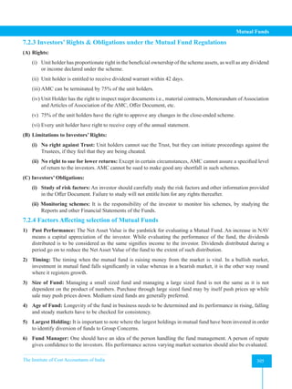
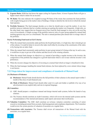
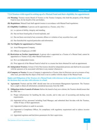
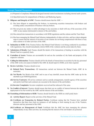
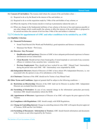
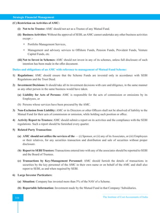
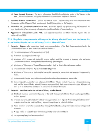
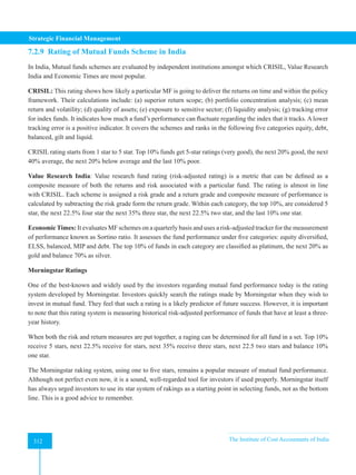
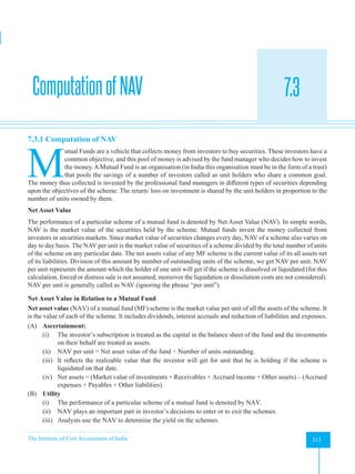
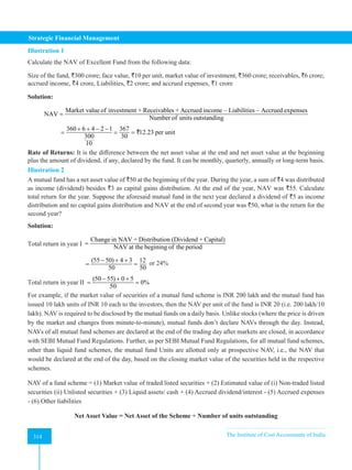
![The Institute of Cost Accountants of India 315
Mutual Funds
Illustration 3
Mr. Ajay on 1.7.2019, during the initial offer of some Mutual Fund invested in 10,000 units having face value of
`10 for each unit. On 31.3.2020 the dividend operated by the M.F. was 10% and Mr. Ajay found that his annualized
yield was 153.33%. On 31.12.2021, 20% dividend was given. On 31.3.2022 Mr. X redeemed all his balance of
11,296.11 units when his annualized yield was 73.52%. What are the NAVs as on 31.3.2020, 31.12.2021 and
31.3.2022?
Solution:
Annualized Return = % Return from date of investment to the date on which annualized return is given or
calculated ÷ Period of the above return in terms of years.
31.3.2020:
Annualized Return = Return from 1.7.2019 to 31.3.2020 / 0.75 year
or, 153.33 = Return from 1.7.2019 to 31.3.2020 / 0.75 year
Return from 1.7.2019 to 31.3.2020 = 115%
It means the investment made on 1.7.2019 has grown to ` 2,15,000 on 31.3.2020
Let the NAV = X
X = [10,000 units + (Amount of dividend/X)] X = 2,15,000
[10,000 units + (`10,000/X)] X = 2,15,000
NAV = 20.50
Total no. of units = 10487.80
31.12.2021
No of units issued (reinvestment of dividend as on 31.12.2021) :
11296.11- 10487.80 = 808.20
NAV = [10487.80 × Dividend per share ] /808.20
= [10487.80 × 2] /808.20 = 25.95
31.3.2022
Annualized Return = Return from 1.7.2019 to 31.3.2022 / 2.75 year
73.52 = Return from 1.7.2019 to 31.3.2021 / 2.75 year
Return from 1.7.2000 to 31.3.2003 = 202.18
It means the investment of `1,00,000 made on 1.7.2000 has grown to `3,02,180 on 31.3.2022.
NAV = 302180 / 11296.11 = 26.75](https://image.slidesharecdn.com/strategyfamous-230209132502-a14bc8e7/85/Strategy_Famous-pdf-327-320.jpg)
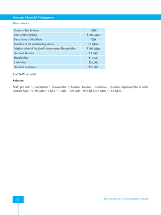
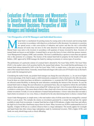
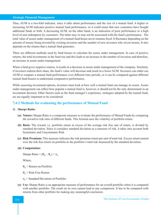
![The Institute of Cost Accountants of India 319
Mutual Funds
2) Treynor’s Ratio:
(a) Nature: Treynor Ratio is a measure to evaluate the performance of mutual funds by comparing the reward
to volatility ratio of different funds. Risk considered here is only Systematic Risk, and not Total Risk.
(b) Assumption: It assumes a completely diversified portfolio, i.e. that the investor would have eliminated all
the unsystematic risk by holding a diversified portfolio.
(c) Basis: Excess return earned over the risk free return on portfolio to the portfolio’s total risk measured by
the Beta of Portfolio. The ratio expresses the portfolio’s risk premium per unit of beta.
(d) Computation:
Treynor’s Ratio = (RP
– RF
) ÷ βP
Where, RP
= Return on Portfolio
RF
= Risk Free Return
βP
= Beta of Portfolio
(e) Use: It is appropriate only in case of comparison with completely diversified portfolio. As in the case of
Sharpe Ratio, Treynor’s measure cannot be used in an isolated manner. It should be compared with such
results of other portfolio to draw conclusions.
3) Jensen’s Alpha:
(a) Nature: It is an absolute measure of evaluating a fund’s performance. It compares desired performance
(based on benchmark portfolio) with actual performance.
(b) Benchmark Performance: Benchmark Performance is computed using Capital Asset Pricing Model
(CAPM), i.e. by factoring the sensitivity of the portfolio return to that the Market Portfolio.
(c) Computation:
Jensen’s Alpha [a] = Actual Return Less Return under CAPM
(d) Evaluation and Appropriateness:
• If Jensen’s Alpha is positive, it reflects that the Mutual Fund has exceeded the expectations and
outperformed the Market Portfolio and vice-versa.
• Alpha would give meaningful results only if its used to compare two portfolios of similar beta factors.
• It is used for measuring performance of a portfolio and to identify the part of the performance that can
be attributed solely to the portfolio.
• This model considers only systematic risk and not the total risk.
Different kinds of expenditure incurred by a Mutual Fund and the way to treat them in computing the net asset
value:
(A) Initial Issue Expenses: AMC incur some expenses when a scheme is launched. The benefits of these
expenses accrue over many years. Therefore, they cannot be charged to any single year. SEBI permits
amortization of initial expenses as follows —](https://image.slidesharecdn.com/strategyfamous-230209132502-a14bc8e7/85/Strategy_Famous-pdf-331-320.jpg)
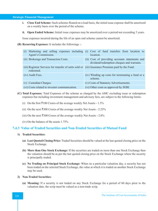
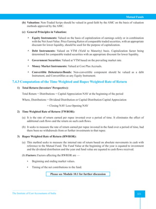
![Strategic Financial Management
322 The Institute of Cost Accountants of India
322
Illustration 5
Chintamani Fund, a fund which invests exclusively in Public Sector Undertakings, yielded `3.75 per Unit for the
year. The opening NAV was `21.20. Chintamani Fund has a risk factor of 3.50%.
Ascertain the Sharpe Ratio and evaluate the funds performance in juxtaposition with performance of the Sensex
if —
(a) Risk Free Return is 5%, Return on Sensex is 15% with a standard deviation of 2.75%.
(b) Risk Free Return is 4%, Return on Sensex is 17% with a standard deviation of 3%.
(c) Risk Free Return is 7%, Return on Sensex is 18% with a standard deviation of 4%.
Solution:
1. Formula for Computing Sharpe Ratio.
Sharpe Ratio = (RP
- RF
) ÷ σp
Where, RP
= Return on portfolio
RF
= Risk Free Return
σP
= Standard Deviation of Portfolio
Particulars Case A Case B Case C
Risk Free Return [RF
] 5% 4% 7%
Market Return [RM
] 15% 17% 18%
Standard Deviation of Market
Return [σM
]
2.75% 3.00% 4.00%
Sharpe Ratio for Chintamani
Fund [(RP
-RF
) ÷ σp
] [A]
3.63
[(17.69% - 5%)÷ 3.50%]
3.91
[(17.69% -4%) ÷ 3.50%]
3.05
[(17.69% -7%) ÷ 3.50%]
Sharpe Ratio for Market
Return [(RM
- RF
)- σM
] [B]
3.64
[(15% - 5%) ÷ 2.75%]
4.33
[(17%-4%) ÷ 3% ]
2.75
[(18% -7%) ÷ 4%]
Sharpe Ratio is Higher for Market Return Market Return Chintamani Fund
Inference / Evaluation Market has outperformed
Chintamani Fund’s
performance.
Market has outperformed
Chintamani Fund’s
performance.
Chintamani Fund has
outperformed Market’s
performance.
Note: Return on Chintamani Fund = Yield ` 3.75 ÷ Opening NAV ` 21.20 = 17.69%.
Illustration 6
Four friends S, T, U, and V have invested equivalent amount of money in four different funds in tune with their
attitude to risk, S prefers to play aggressive and is keen on equity-funds, T is moderately aggressive with a desire
to invest upto 50% of his funds in Equity, whereas U does not invest anything beyond 20% in Equity. V, however,
relies more on movement of market, and prefers any fund which replicates the market portfolio.
Their investment particulars, returns therefrom and Beta of the fund are given below —](https://image.slidesharecdn.com/strategyfamous-230209132502-a14bc8e7/85/Strategy_Famous-pdf-334-320.jpg)
![The Institute of Cost Accountants of India 323
Mutual Funds
Fund Invested Return for the year Beta Factor
Money Multiplier Fund (100% Equity) 23.50% 1.80
Balanced Growth Fund (50% Equity - 50% Debt) 16.50% 1.25
Safe Money Fund (20% Equity and 80% Debt Funds) 12.50% 0.60
If the Market Return was 16% and the Risk Free Return is measured at 7%, which of the four friends were rewarded
better per unit of risk taken?
Solution:
Particulars S T U V
Risk Free Return [RF
] 7% 7% 7% 7%
Fund Invested Money Multiplier
Fund
Balanced Growth
Fund
Safe Money
Fund
Market
Portfolio
Beta of the Portfolio [βP
] 1.80 1.25 0.60 1.00
Return on Portfolio [RP
] 23.50% 16.50% 12.50% 16.00%
Treynor Measure [(RP
-RF
) ÷ βP
] 9.17
[23.50–7] ÷1.80
7.60
[16.50–7] ÷ 1.25
9.17
[12.50–7] ÷ 0.60
9.00
[16–7] ÷ 1
Ranking 1 3 1 2
Evaluation: Both S and U have earned the same Reward per unit of risk taken, which is more than the Market
Reward to Risk of 9.00.
Illustration 7
Following information is available regarding four mutual funds:
Mutual Fund Return Risk (σ) β (Beta) Risk free rate
P 13 16 0.90 10
Q 17 23 0.86 10
R 23 39 1.20 10
S 15 25 1.38 10
Evaluate performance of these mutual funds using Sharp Ratio and Treynor’s Ratio. Comment on the evaluation
after ranking the funds.
Solution:
Mutual
Fund
Under Sharpe’s Method
[(RP
-RF
) ÷ σP
]
Ranking
Under Treynor
Method
[(RP
-RF
) ÷ βP
]
Ranking
P [(13-10) ÷ 16] = 0.19 4 [(13-10) ÷ 0.90] = 3.33 4
Q [(17-10) ÷ 23] = 0.31 2 [(17-10) ÷ 0.86] = 8.14 2
R [(23-10) ÷ 39] = 0.33 1 [(23-10) ÷ 1.20] = 10.83 1
S [(15-10) ÷ 25] = 0.2 3 [(15-10) ÷ 1.38] = 3.63 3](https://image.slidesharecdn.com/strategyfamous-230209132502-a14bc8e7/85/Strategy_Famous-pdf-335-320.jpg)
![Strategic Financial Management
324 The Institute of Cost Accountants of India
324
Illustration 8
The following particulars are furnished about three Mutual Fund Schemes, P, Q and R
Particulars Scheme P Scheme Q Scheme R
Dividend Distributed `1.75 — `1.30
Capital Appreciation `2.97 `3.53 `1.99
Opening NAV `32.00 `27.15 `23.50
Beta 1.46 1.10 1.40
Ascertain the Alpha of the three schemes and evaluate their performance, if Government of India Bonds carry an
interest rate of 6.84% and the NIFTY has increased by 12.13%.
Solution:
Particulars Scheme P Scheme Q Scheme R
Dividend Distributed `1.75 - `1.30
Add: Capital Appreciation `2.97 `3.53 `1.99
Total Return [A] `4.72 `3.53 `3.29
Opening NAV [B] `32.00 `27.15 `23.50
Actual Return [A] ÷ [B] = [C] 14.75%
[4.72 ÷32.00]
13.00%
[3.53 ÷ 27.15]
14.00%
[3.29 ÷ 23.50]
Beta [D] 1.46 1.10 1.40
Expected Return under CAPM [E(RP
)] [E]
RF
+ βP
X (RM
– RF
) = 6.84 + [D] × (12.13 - 6.84)
14.56%
[6.84 + 1.46 ×
(12.13 – 6.84]
12.66%
[6.84 + 1.10 ×
12.13 – 6.84]
14.25%
[6.84 + 1.40 ×
(12.13 – 6.84]
Jensen’s Alpha (σp
) [C] – [E] 0.19% 0.19%
(14.75-14.56)
0.34%
(13.00-12.66)
(0.25%)
(14.00-14.25)
Ranking 2 1 3](https://image.slidesharecdn.com/strategyfamous-230209132502-a14bc8e7/85/Strategy_Famous-pdf-336-320.jpg)
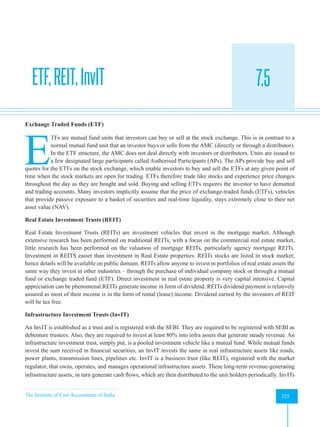
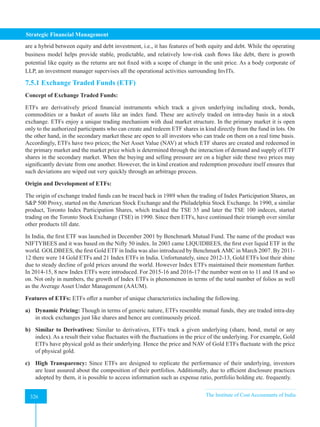
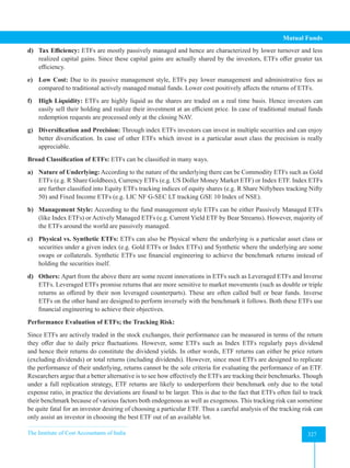
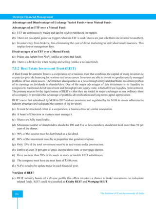
![Strategic Financial Management
334 The Institute of Cost Accountants of India
334
Additional Illustrations
1. Mr. Shyam invested in a mutual fund when the NAV was `12.65 per unit. 60 days later the asset value per
unit of the fund was `12.25. In the meantime, Shyam had received a cash dividend of `0.50 and a capital gain
distribution of `0.30. Compute the monthly return.
Solution:
[Divided + Capital gain distribution + Capital appreciation] / Opening NAV
= (0.50 + 0.30 – 0.40)/12.65 = 3.16%
Annualized return = (Return × 365)/60 days = 19.22% p.a.
Monthly return = 19.22/12 or 1.60% p.m.
2. Mr. Sharma can earn a return of 16% by investing in equity shares of his own. Now he is considering a
recently announced equity-based mutual fund scheme in which initial expenses are 5.7 percent and annual
recurring expenses are 1.7 percent. How much should the mutual fund earn to provide Mr. Sharma a return of
16 percent?
Solution:
Let the return on mutual fund be `X.
Investor’s expectation denotes the return from the amount invested.
Returns from mutual funds =
Investor's expectations
100 – Issue expectations + Annual recuring expenses
X =
16
1.7
1 0.057
+
−
= 16.96 + 1.7 = 18.67%
The Mutual Fund should earn so as to provide a return of 16% = 18.67%.
3. You have purchased 2000 shares of India Hope Fund which had a net asset value of `10.00 per unit at the
beginning of the year. The fund deducted a front-end load of 5%. The securities in the fund increased in value
by 10% during the year. The fund’s expense ratio is 1.1%. What is your rate of return on the fund if you sell
your shares at the end of the year?
Solution:
Initial investment = (`10×2000)/0.95 = `21052.63.
The ending value of the shares includes the increase of 10% minus the expense ratio of 1.1%
Ending value = `20,000 × (1.10-0.011) = `21,780.
The returns are equals to:
(Ending value – Beginning value) – 1 = (`21780.00/21052.63) –1 = 3.46%
4. You are considering an investment of `5,000 in a mutual fund with a 6% load and an annual expense ratio of
0.8%. You plan to invest for five years. Assume the portfolio rate of return net of operating expenses is 10%
annually. What is the value of portfolio after five years?](https://image.slidesharecdn.com/strategyfamous-230209132502-a14bc8e7/85/Strategy_Famous-pdf-346-320.jpg)
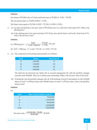
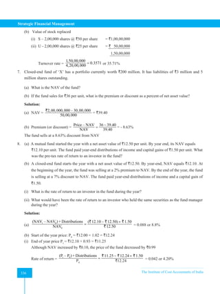
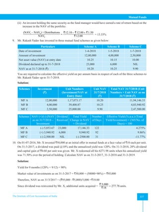
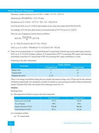
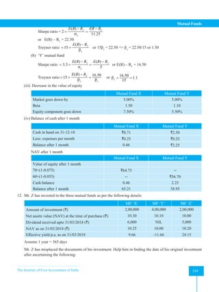
![Strategic Financial Management
340 The Institute of Cost Accountants of India
340
(i) Number of units in each scheme
(ii) Total net present value
(iii) Total yield
(iv) Number of days of investment held
Solution:
(i) Number of units in each scheme
MF ‘X’ 2,00,000
19,417.48
10.30
=
`
`
MF ‘Y’ 4,00,000
39,603.96
10.10
=
`
`
MF ‘Z’ 2,00,000
20,000.00
10.00
=
`
`
(ii) Total NAV as on 31/3/2018
MF ‘X’ 19,417.48 × `10.25 = `1,99,029.17
MF ‘Y’ 39,603.96 × `10.00 = `3,96,039.60
MF ‘Z’ 20,000 × `10.20 = `2,04,000.00
`7,99,068.77
(iii) Total yield
Name of Mutual Funds Capital Yield Dividend Yield Total
MF ‘X’ `1,99,029.17 - `2,00,000 = - `970.83 `6,000 `5,029.17
MF ‘Y’ `3,96,039.60 - `4,00,000 = - `3,960.40 NIL -3,960.40
MF ‘Z’ `2,04,000 - `2,00,000 = `4,000 `5,000 `9,000.00
Total 10,068.77
Total yield =
10068.77
100 1.2586%
8,00,000
× =
`
`
(iv) No. of days investment was held
MF ’X’ MF ‘Y’ MF ‘Z’
Let number of days be X Y Z
Initial Investment 2,00,000 4,00,000 2,00,000
Yield (`) 5029.17 -3960.40 9,000
Yield (%) 2.5146 -0.9901 4.5
Period of holding (Days) (2.5146 ÷ 9.66) ×
365 = 95 days
[(-0.9901) ÷ (-11.66)] ×
365 = 31 days
(4.5 ÷ 24.15) ×
365 = 68 days
Date of Original Investment 26.12.17 28.02.18 22.01.18](https://image.slidesharecdn.com/strategyfamous-230209132502-a14bc8e7/85/Strategy_Famous-pdf-352-320.jpg)
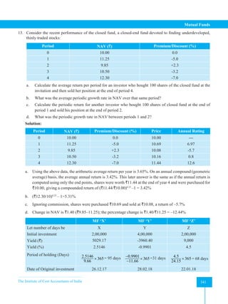
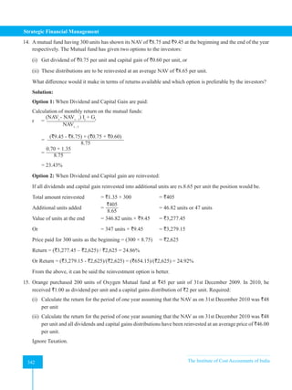
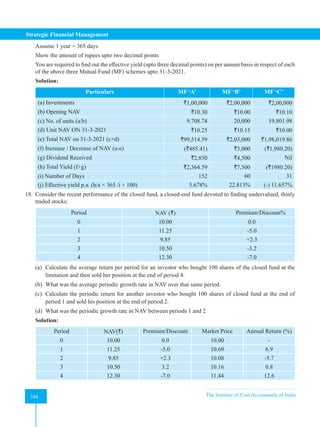
![The Institute of Cost Accountants of India 345
Mutual Funds
a. Using the above data, the arithmetic average return per year is 3.65%. On an annual compound (geometric
average) basis, the average annual return is 3.42%.
This latter answer is the same as if the annual return is computed using only the end points, shares
were worth `11.44 at the end of year 4 and were purchased for `10.00, giving a compounded return of
(`11.44/`10)0.25 – 1 = 3.42%
b. (`12.30/10)0.25 – 1 = 5.31%
c. Ignoring commission, shares were purchased `10.69 and sold at `10.08, return of – 5.7%
d. Change in NAV is ` -1.40 (` 9.85-11.25); the percentage change is ` -1.40/`11.25 = 12.44%
Solved Case Studies
1. Summer Mutual Fund sponsored open-ended equity-oriented fund.
There were three plans size ‘S’, dividend reinvestment plan; ‘T’, bonus plan and ‘U’, growth plan.
At the time of initial public offer on 1-4-2011, Mr. Sachin, Mr. Sourav and Mr. Rahul, three investors invested
`1,00,000 each and chosen ‘T’, ‘U’ and ‘S’ plans, respectively.
The history of the fund is as follows:
Dividend (%) Bonus Ratio Net Asset Value Per Unit (`10)
Plan S Plan T Plan U
28-07-2015 20 -- 30.70 31.40 33.42
31-03-2016 70 5:4 58.42 31.05 70.05
31-10-2019 40 -- 42.18 25.02 56.15
15-03-2020 25 -- 46.45 29.10 64.28
31-03-2020 -- 1:3 42.18 20.05 60.12
31-03-2021 40 1:4 48.10 19.95 72.40
31-07-2021 -- -- 53.75 22.98 82.07
[Ignore Education Cess]
On 31st
July, 2021, all three investors redeemed all the balance units. Calculate the annual rate of return to each
of the investors consider:
(i) Long-term capital gain is exempt from income tax.
(ii) Short-term capital gain is subject to income tax @ 10%.
(ii) Security transaction tax is 0.2 percent only on sale/redemption of units.](https://image.slidesharecdn.com/strategyfamous-230209132502-a14bc8e7/85/Strategy_Famous-pdf-357-320.jpg)
![Strategic Financial Management
346 The Institute of Cost Accountants of India
346
Solution:
Return from plan ‘S’ – dividend reinvestment for Rahul. Under dividend reinvestment plan, the amount of
dividend is reinvested in the business at the prevailing rate.
(a) Statement of units, value and return on investment
Date
Dividend
(%)
Investment
(`)
Rate
(`)
Units
Commutative
Units
Value
(`)
(1) (2) (3) = Div × Cum. Units (4) (5) = (3)/(4) (6) (7) = 6×`10
01-04-2011 Initial offer 1,00,000 10.00 10,000.00 10,000.00 1,00,000
28-07-2015 0.20 20,000
(2×10,000)
30.70 651.47 10,651.47 1,06,515
31-03-2016 0.70 74,560
(7×10,651.47)
58.42 1,276.28 11,927.75 1,19,278
31-03-2019 0.40 47,711
(4×11,927.75)
42.18 1,131.13 13,058.88 1,30,589
15-03-2020 0.25 32,647
(2.5×13,058.88)
46.45 702.85 13,761.73 1,37,617
24-03-2021 0.40 55047
(4×13,761.33)
48.10 1,144.43 14,906.16 1,49,062
31-07-2021 — — 53.75 — 14,906.16 1,49,062
(b) Return on Investment
Particulars `
Redemption value = 14,906.16 × 53.75 8,01,206.10
Less: Short-term capital gain tax @ 10% = 1,144.43 units (53.75 - 48.10) × 10% 646
8,00,560.10
Less: Securities transaction tax @ 0.2% on `8,01,206.10 1,602.41
Redemption value net of taxes 7,98,957.69
Less: Investment 1,00,000.00
Net return from investment 6,98,957.69
Period of investment (1/4/2011 to 31/07/2021) in months 124
Annual average return =
[Net Return × 12 months × 100]
Purchase price × Period of investment (in months)
=
6,98,957.69 × 12 × 100
1,00,000 × 124 67.64%
Short-term capital gains is only in respect of investment made on 24-3-2021 where the period of holding is less
than 1 year. Securities transaction tax is not to be considered for short-term capital gains and hence deducted
from the net amount to ascertain cash flows.](https://image.slidesharecdn.com/strategyfamous-230209132502-a14bc8e7/85/Strategy_Famous-pdf-358-320.jpg)
![The Institute of Cost Accountants of India 347
Mutual Funds
Returns from Plan ‘T’ – Bonus plan for Mr. Sachin and under the bonus plan, bonus units are issued in the
specified ratio.
(a) Statement of units, bonus and value per unit
Date Bonus Ratio Units Cum. Units NAV/Unit (`)
(1) (2) (3) (4) (5)
01-04-2011 Initial issue 10,000 10,000 10.00
31-03-2016 5:4 12,500 (10,000×5/4) 22,500 31.05
31-03-2020 1:3 7,500 (22,500×1)/3 30,000 20.05
24-03-2021 1:4 7,500 (30,000×1)/4 37,500 19.95
(b) Return on Investment
Particulars `
Redemption value = 37,500 × 22.98 8,61,750.00
Less: Short-term capital gain tax @ 10% = 7500 ×(22.98 - 0)× 10% 17,235.00
8,44,515.00
Less: Securities transaction tax @ 0.2% 1,723.50
Net of tax 8,42,791.50
Less: Investment 1,00,000.00
Net gain 7,42,791.50
Annual average return =
[Net Return × 12 months × 100]
Purchase price × Period of investment (in months)
=
7,42,719.50 × 12 × 100
1,00,000 × 124 71.88%
(i) For income tax purposes, cost of acquisition of bonus shares is considered as NIL.
(ii) Short-term capital gains is only in respect of bonus issued on 24-3-2016 as the period of holding is less
than 1 year.
Return from plan U - Growth plan to Mr. Sourav
Particulars `
Redemption value (10,000 × 82.07) 8,20,700.00
Less: Security transaction tax (S.T.T) is 0.2% 1,641.40
Net amount received 8,19,058.60
Less: Investment 1,00,000.00
7,19,058.60
There is no short-term capital gains as the period of holding is more than 1 year
Average annual return = [(7,19,058.60 × 12 × 100)] ÷ [(1,00,000 × 124)] = 69.59%](https://image.slidesharecdn.com/strategyfamous-230209132502-a14bc8e7/85/Strategy_Famous-pdf-359-320.jpg)
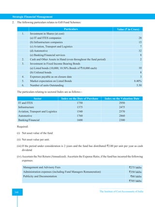
![The Institute of Cost Accountants of India 349
Mutual Funds
Solution:
(1) Net asset value of the fund
Particulars ` in Crore
1. Market value of shares in
(a) IT and ITES [Cost `28×Closing Sector Index 2950÷Opening Sector Index 1750] 47.20
(b) Infrastructure [Cost `15×Closing Sector Index 2475÷Opening Sector Index 1375] 27.00
(c) Aviation [Cost `7×Closing Sector Index 2570÷Opening Sector Index 1540] 11.68
(d) Automotive [Cost `32×Closing Sector Index 2860 ÷ Opening Sector Index 1760] 52.00
(e) Banking [Cost `8×Closing Sector Index 2300÷Opening Sector Index 1600] 11.50
2. Market Value of Investment in Listed Bonds [(Face value `10 crores × Interest on
Face Value @10.50%) ÷ Market Expectation 8.40%]
12.50
3. Cost of investment in Unlisted Bonds 8.00
4. Cash and Other Assets 2.00
Total Assets of the fund
Less: Outstanding Expenses
171.88
(3.00)
Net Asset Value of the Fund 168.88
Note: It is assumed that Cash and Other Assets existed from the beginning of the period at the same
values.
(2) Net asset value per unit
NAV Per Unit = Net Asset Value of the Fund ÷ No. of units outstanding
= `168.88 crore ÷ 5.50 crore units = `30.71
(3) Annualized return on Fund
(a) Computation of Opening NAV
Particulars ` in crore
1. Investment in Shares (at Cost)
(a) IT and ITES Companies 28.00
(b) Infrastructure Companies 15.00
(c) Aviation, Transport and Logistics 7.00
(d) Automotive 32.00
(e) Banking/Financial Services 8.00
2. Investment in Fixed Income Bearing Bonds
(a) Listed Bonds [10,000; 10.50% bonds of `10,000 each] 10.00
(b) Unlisted Bonds 8.00
Net Asset Value 108.00
Note: Cash and Other Assets are not included because they arise out of investments made in the beginning.](https://image.slidesharecdn.com/strategyfamous-230209132502-a14bc8e7/85/Strategy_Famous-pdf-361-320.jpg)
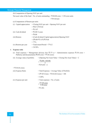
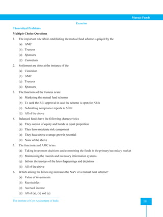
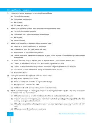


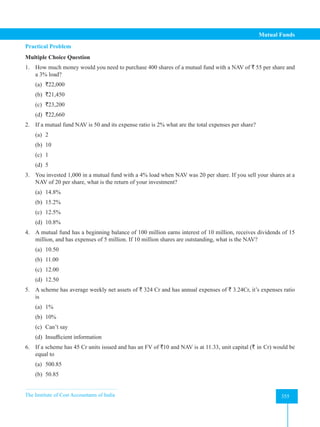
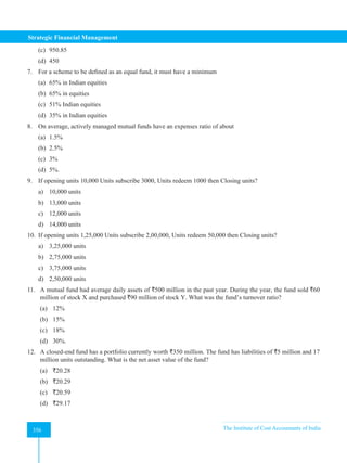
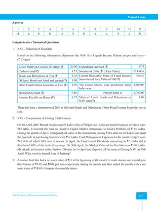
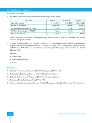

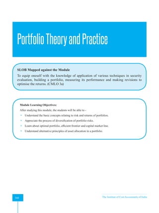
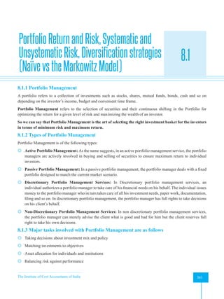
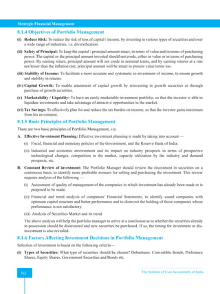
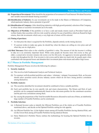
![Strategic Financial Management
364 The Institute of Cost Accountants of India
364
4. Portfolio Revision:
(a) Portfolio Monitoring and Revision is intended to ensure that the Portfolio does not lose it optimality.
(b) The need for revision arises due to: (i) market-related changes, e.g. change in risk-return patterns, economy
changes, emergence of new securities, or (ii) investor-related changes, e.g. availability of additional funds
for investment, change in risk appetite, need of cash for other alternative use, etc.
(c) Portfolio Revision should be carried out with care, scientifically and objectively, and is as important as
Portfolio Analysis and Selection.
5. Portfolio Evaluation:
(a) This involves assessing the risk-return performance of the portfolio over a period, by quantitative
measurement of actual return realized and the risk borne by the portfolio over the period of investment.
(b) This provides a mechanism for identifying weaknesses in the investment process and for overcoming
them.
Note: Portfolio Management is an ongoing process, achieved through continual refinement of skills and market
watch.
8.1.8 Portfolio Return and Risk
8.1.8.1 Portfolio Return
Harrry Markowitz, the father of modern portfolio theory, published an article in the Journal of Finance in March
1952. It was the first scientific approach to determine the risk return, covariance of the securities and developed a
methodology for determining the optimum portfolio. Before Markowitz, it was the knowledge of smart investors,
i.e., the traditional theory that ‘don’t put all the eggs into a single basket.’ That represents the risk diversification
without adequate scientific knowledge about risk. Individual securities have risk return characteristics of their own.
But portfolios which are combination of securities do not take the aggregate characteristics of risk and return in
the same direction as compared to their individual parts. In recognition for his contribution in the field of finance,
Harry Markowitz was awarded Nobel Prize in Economics in the year 1990.
Concept of Return We can calculate the portfolio’s expected return using historical data or using the probability
of future returns of the securities. Portfolio theory is primarily concerned with the ex-ante (future) events which
indicate expected future results. All portfolio decisions are for future, and hence we should consider ex-ante values.
On the other hand, if we want to evaluate the portfolio performance, we should calculate the actual return and risk
for past periods, i.e, ex-post values. It is very important to understand that ex-ante values which will always be the
projected values and ex-post values will always be actual values of past results.
Measurement of historical returns: Any historical return may be calculated as Holding Period yield.
[(Share price at the end of year - Share price at the beginning of the
year) +Dividend received]/(Share price at the beginning of the year)
Illustration 1
Mr. Amit bought 10 shares of TCS on 1.4.2018 for ` 30,050. The company paid a dividend of `30 per share and the
value of the stock as on 31.3.2019 was `34,280. Calculate the holding period yield of the investor.](https://image.slidesharecdn.com/strategyfamous-230209132502-a14bc8e7/85/Strategy_Famous-pdf-376-320.jpg)
![The Institute of Cost Accountants of India 365
Portfolio Theory and Practice
Solution:
Holding period return: = [(` 34,280 - `30,050) + `300]/(`30,050) = 15.07%.
It is better to split it into two parts (a) Current yield; and (b) Capital appreciation.
Current yield = (Dividend received)/(Initial investment)
= (`300)/(`30,050)
= 0.00998
Capital appreciation = (Closing value-Opening value )/(Initial investment)
= (`34,280 - `30,050)/(`30,050)
= 0.14076
Total yield = 0.00998 + 0.14076 = 15.07%.
We can find out the historical return of a portfolio by considering the respective weights attached to it and the
combined portfolio weights will be equal to one or hundred percent.
E(RP
) = Ʃ
n
i=1
Wi
(Ri
)
Illustration 2
A portfolio manager invests in five portfolios namely P, Q, R, S and T in the ration of 30%, 20%, 25%, 15% and
10% and the respective returns of the portfolios are 12%, 14% - 20%, 10% and 9%.
The combined portfolio return will be:
Solution:
RP = 0.30 × 0.12 + 0.20 × 0.14 + 0.25 × -0.20 + 0.15 × 0.10 + 0.10 × 0.09
= 0.036 + 0.028 – 0.05 + 0.015 + 0.009
= 3.8%.
Ex-ante Return of a Portfolio
Ex-ante return will always be the projected or future returns. We are putting probability factor to determine the
future expected value. The future expected returns of the portfolio may be calculated as the probability multiplied
by the returns of individual securities.
Ex-ante return of a portfolio = ƩPi
Ri
Illustration 3
Calculate the return of a portfolio which has 60% invested in TCS and the rest in RIL. The probable return in
different conditions of the economy are as follows:
Condition of the economy Probability of occurrence (%) Return on TCS(%) Return of RIL(%)
Growth 50 16 12
Stable 40 12 14
Recession 10 -6 -2
Find out only the return of the portfolio.](https://image.slidesharecdn.com/strategyfamous-230209132502-a14bc8e7/85/Strategy_Famous-pdf-377-320.jpg)
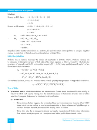
![The Institute of Cost Accountants of India 367
Portfolio Theory and Practice
(ii) Interest Rate Risk
• Uncertainty of future market values and extent of income in the future, due to fluctuations in the
general level of interest, is known as Interest Rate Risk.
• These are risks arising due to fluctuating rates of interest and cost of corporate debt. The cost of
corporate debt depends on the interest rates prevailing, maturity periods, credit worthiness of the
borrowers, monetary and credit policy of RBI, etc.
(iii) Purchasing Power Risk: Purchasing Power Risk is the erosion in the value of money due to the effects
of inflation.
B. Unsystematic Risk: These are risks that emanate from known and controllable factors, which are unique and/
or related to a particular security or industry. These risks can be eliminated by diversification of portfolio.
(i) Business Risk
• It is the volatility in revenues and profits of particular Company due to its market conditions, product
mix, competition, etc.
• It may arise due to external reasons or (Government policies specific to that kind of industry) internal
reasons (labour efficiency, management, etc.)
(ii) Financial Risk
• These are risks that are associated with the Capital Structure of a Company. A Company with no Debt
Financing, has no financial risk. Higher the Financial Leverage, higher the Financial Risk.
• These may also arise due to short term liquidity problems, shortage in working capital due to funds
tied in working capital and receivables, etc.
(iii) Default Risk: These arise due to default in meeting the financial obligations on time. Non- payment of
financial dues on time increases the insolvency and bankruptcy costs.
C. Risk Involved In Investment in Government Securities [G. Sec.]
Interest Rate Risk
(i) Interest Rate Risk are on account of inverse relation of price and interest. These are typical of any fixed
coupon security with a fixed period to maturity.
(ii) However, this risk can be completely eliminated in case an investor’s investment horizon (intended period
of holding) identically matches the term of security.
Re-investment Risk
(i) Re-investment risk is the risk that the rate at which the interim cash flows are re-invested may fall thereby
affecting the returns.
(ii) The most prevalent tool deployed to measure returns over a period of time is the yield-to- maturity (YTM)
method which assumes that the cash flows generated during the life of a security is reinvested at the rate
of YTM.
Default Risk
(i) Default risk in the context of a Government Security is always zero.
(ii) However, these securities suffer from a small variant of default risk, i.e. maturity risk.](https://image.slidesharecdn.com/strategyfamous-230209132502-a14bc8e7/85/Strategy_Famous-pdf-379-320.jpg)
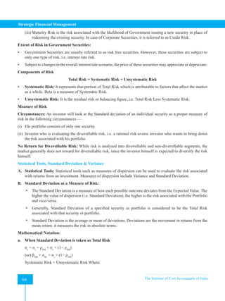
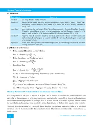
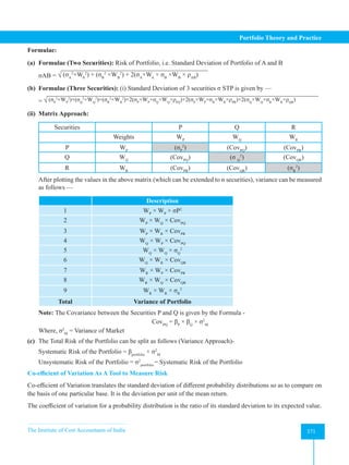
![Strategic Financial Management
372 The Institute of Cost Accountants of India
372
Illustration 4
Two securities A and B have a standard deviation of 10% and 20% each. On first glance, Security B is more riskier
than Security A. If mean (average) returns of Securities A and B is 10% and 30% respectively, then we can observe
that A has more risk per unit of return, while B has a lower risk per unit of return.
Solution:
Particulars Security A Security B
Standard Deviation 10% 20%
Mean Return (Average Expected Return) 10% 30%
Co-Efficient of Variation [Standard Deviation ÷ Average Return] 10% ÷ 10% = 1 20% ÷ 30% = 0.67
Purpose:
Standard Deviation measures the dispersion in absolute terms. It does not provide a base for comparison. Coefficient
of variance provides a common base. i.e. extent of variance, which can be used to compare different investments.
Formula:
Co-efficient of Variation = Standard Deviation ÷ Expected NPV
Meaning of covariance it is the relationship or responsiveness of returns between two securities – how they move
or change each other. It is the product of deviations of returns from their arithmetic mean. It is calculated as
follows:
(a) When historical data is given:
1
( ) ( )
A A B B
R R R R
N
∑ − −
where RA
denotes return from security A, RB
denotes return from security B, A
R , is the arithmetic mean of
returns from security A, B
R , is the arithmetic mean of returns from security B, N = No. of terms.
(b) When probability or ex-ante data is used the formula will be
1
( ) ( ).
n
i iA A iB B
i
P R R R R
=
− −
∑
Illustration 5
The return in two securities and their associated probabilities are given below. Find out the value of (r), i.e.,
correlation coefficient.
State of economy Probability Return of security X (%) Return of security Y (%)
1 0.20 12 15
2 0.30 15 12
3 0.10 -7 15
4 0.25 11 -4
5 0.15 7 6](https://image.slidesharecdn.com/strategyfamous-230209132502-a14bc8e7/85/Strategy_Famous-pdf-384-320.jpg)
![The Institute of Cost Accountants of India 373
Portfolio Theory and Practice
Solution:
Calculation of covariance
State of
economy
Probability Return on
Security X
(%)
Return of
Security
Y (%)
Deviation of
return of security
X from it mean
Deviation of
return of security
Y from its mean
Product of the
deviation X
probability
(1) (2) (3) (4) (5) (6) (7)
1 0.20 12 15 12-10 = 2 15–8 = 7 2.80
2 0.30 15 12 15-10 = 5 12–8 = 4 6.00
3 0.10 –7 15 –7–10 = –17 15–8 = 7 –11.9
4 0.25 11 –4 11–10 = 1 –4 –8 = –12 –3.0
5 0.15 7 6 7–10 = –3 6–8 = –2 0.9
Sum = –5.2
The expected return on security X:
= E(Rx
) = (0.20 × 12) + (0.30 ×15) + (0.10 × –7) + (0.25 × 11) + (0.15 × 7)
= 2.4 + 4.5 – 0.70 + 2.75 + 1.05 = 10%
The expected return on security Y:
= E(Ry
) = (0.20 × 15) + (0.30 ×12) + (0.10 × 15) + (0.25 × –4) + (0.15 × 6)
= 3.00 + 3.6 + 1.5 – 1.00 + 0. = 8%
Covariance between the returns of securities is – 5.2.
We have to calculate the S.D. of X and S.D. of Y respectively to find out the value of (r)
σ2
x
= 0.20 (12-10)2
+ 0.30 (15-10)2
+ 0.10 (-7-10)2
+ 0.25 (11-10)2
+ 0.15 (7-10)2
= 0.20 (4) + 0.30 (25) + 0.10 (289) + .25 (1) + 0.15 (9)
= 0.8 + 7.5 + 28.9 + 0.25 + 1.35 = 38.8.
Or σx
= 6.23%
2
Y
σ = .20 (15 – 8)2
+ 0.30 (12 – 8)2
+ 0.10 (15 – 8)2
+ 0.25 (– 4 – 8)2
+ 0.15 (6 – 8)2
= 0.20 (49) + 0.30 (16) + 0.10 (49) + 0.25 (144) + 0.15 (4)
= 9.8 + 4.8 + 4.9 + 36 + 0.60 = 56.10
or Y
σ = 7.49%.
Covariance may be calculated in this process also:
Cov (X, Y) = [0.20 (12 – 10) (15 – 8) + 0.30 (15 – 10) (12 – 8) + 0.10 (– 7 – 10) (15 – 8)
+ 0.25 (11 – 10) (– 4 – 8) + 0.15 ( 7 – 19) ( 6 – 8)]
= 0.20 (14) + 0.30 (20) + 0.15 (–119) + 0.25 ( –12) + 0.15 (6)
= 2.80 + 6 – 11.90 – 3 + 0.90
= – 5.2.
Correlation coefficient r = [Cov(X, Y)] ÷ [σx
× σY
] = - 5.2 ÷ [6.23 × 7.49]
or r = (- 5.2) ÷ 46.6627 = -0.11.](https://image.slidesharecdn.com/strategyfamous-230209132502-a14bc8e7/85/Strategy_Famous-pdf-385-320.jpg)
![Strategic Financial Management
374 The Institute of Cost Accountants of India
374
Correlation and Diversification
A. Correlation Co-efficient
Correlation Co-efficient is a measure of closeness of the relationship between two random variables and is
bounded by the values +1 and -1.
Different Meaning of Co-relation Coefficient (r)
The value of r varies from -1 to +1. When the value of r is -1, it represents a complete perfect negative correlation
by which we can reduce our portfolio risk to zero, provided the other conditions are satisfied. When the value of r is
zero, it means there is no correlation or co-movement. The returns are independent and still we can reduce our risk.
When the value of r represents +1, it denotes a perfect positive correlation and hence no risk reduction is possible.
Formulae:
The formulae for determining the correlation coefficient are—
(i) Based on Covariance and Standard Deviation:
ρXY
= CovXY
÷ (σX
× σY
)
(ii) Based on Probability Distribution of Future Returns:
ρXY
=
∑[Xi
- E(Xi
)] × [i
- E(Yi
)]
∑R2
M
-nR2
m
(iii) Based on historical realized returns
ρXY
=
n∑Xi
Yi
- ∑Xi
∑Yi
√[n∑Xi
2
-(∑Xi
)2
] - [n∑Yi
2
-(∑Yi
)2
]
Valuation and Inference
Portfolio Risk will be —
(a) Maximum when two components of a portfolio stand perfectly positively correlated.
(b) Minimum when two components of a portfolio stand perfectly negatively correlated.
B. Diversification:
Diversification refers to investing in more than one security, i.e. dividing the Portfolio into different stocks and not
investing the money in one particular stock. Some of the risks associated with individual assets can be eliminated
by forming Portfolio by way of spreading an investment across assets. This is called diversification.
Features:
(i) Diversification reduces risks because prices of different stocks do not move exactly together. It helps to reduce
Portfolio risk by eliminating unsystematic risk for which investors are not rewarded.
(ii) Investors are rewarded for taking market risk.
(iii) Diversification averages the returns of the assets within the Portfolio, thereby it attenuates the potential highs
(and lows).
(iv) Diversification among companies, industries and asset classes, protects against business risk, and financial
risk.](https://image.slidesharecdn.com/strategyfamous-230209132502-a14bc8e7/85/Strategy_Famous-pdf-386-320.jpg)
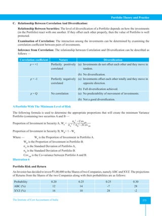
![Strategic Financial Management
376 The Institute of Cost Accountants of India
376
You are required to-
1. Comment on Return and Risk of Investment in Individual Shares.
2. Compare the Risk and Return of these two Shares with a Portfolio of these Shares in equal proportions.
3. Find out the proportion of each of the above Shares to formulate a minimum Risk Portfolio.
Solution:
1. Computation of Expected Returns and Risk of the Individual Shares
P RA
RB
P × RA
P × RB
DA
=RA
–RA
DB
=RB
–RB
P × (DA
)2
P × (DB
)2
P(DA
×DB
)
0.20 12 16 2.40 3.20 0.55 3.90 0.06 3.04 0.43
0.25 14 10 3.50 2.50 1.45 -2.10 0.53 1.10 -0.76
0.25 -7 28 -1.75 7.00 -19.55 15.90 95.55 63.20 -77.71
0.30 28 -2 8.40 -0.60 15.45 -14.10 71.61 59.64 65.35
RA
=12.55% R B
=12.10% σ2
A
=167.75 σ2
B
= 126.98 -143.39
Standard Deviation = σA
= √167.75 = 12.95%, Standard Deviation = σB
= √126.98 = 11.27%
Computation of Co-efficient of Variation (Risk per unit of Return):
For ABC: 12.95 ÷ 12.55 = 1.03 For XYZ: 11.27 ÷ 12.10 = 0.93
Conclusion: Hence, based on Risk, XYZ is more preferable.
2. Risk and Return of the Portfolio (50% : 50% mix)
(a) Return of the Portfolio: Returns in %: (12.55 × 0.50) + (12.10 × 0.50) = 12.325%
Returns in Amount: 1000.000 × 12.325 = `12,325
(b) Risk of the Portfolio-Standard Deviation of the Portfolio (Matrix Approach):
WABC
(0.05) WXYZ
(0.05)
WABC
(0.05)
= 0.5 × 0.5 × σABC
2
= 0.25 × (12.95)2
= 41.9256
0.5 × 0.5 × Cov(XYZ, ABC
)
= 0.25 × (-144.255) = -36.0638
σABC XYZ
2
= 41.9256+31.7532+2 × (-36.0638)
= 1.5512%
WXYZ
(0.05)
= 0.5 × 0.5 × Cov. (XYZ, ABC
)
= 0.25 × (-144.255) = 36.0638
0.5 × 0.5 × σ XYZ
2
= 0.25 × (11.27)2
= 31.7532
σ ABC XYZ
2
= 1.245%
So, Minimum Risk Portfolio WABC
= [σXYZ
2
- COV(ABC XYZ
)]/[(σABC
2
+ σXYZ
2
-2COV(ABC XYZ
)]
= [(11.27)2
- (-143.39)]/[(12.95)2
+ (11.27)2
- 2(-143.39)]
WABC
= 46.50% (Proportion of Investment in ABC share)
WXYZ
= 100% - WABC
= 53.50% (Proportion of investment in XYZ share)](https://image.slidesharecdn.com/strategyfamous-230209132502-a14bc8e7/85/Strategy_Famous-pdf-388-320.jpg)
![The Institute of Cost Accountants of India 377
Portfolio Theory and Practice
Expected Return of A Security Under Sharpe Single Index Market Model
Market Model: Market Model does not pre-suppose the existence of risk free return for the purpose of estimating
return from a security. Under this model (assumption), the market risk affects the whole of return from a security,
and not just the return in excess of the risk-free rate.
Formulae:
1. Expected Return [E(RP
)]: Without considering Risk Free Return
→E(RP
) = αP
+(βP
×RM
)+ e
Components:
Notation Description
αP
(Alpha Intercept) It is the return from a Security / Portfolio when Market Return is Zero.
= Average Return Less Expected Return (Beta Adjusted Return) = Rp
- βP
× RM
Over a longer period, α should be Zero.
βP
× RM
Beta Adjusted Market Return.
e Error Factor (with Zero Mean and constant standard deviation)
2. Expected Return: Considering Risk Free Return (Risk Adjusted Excess Return Approach)
→ E(RP
) = αP
- [R ×(1-βP
)] + RF
+ [βP
(RM
- RF
)] + e
Components:
Notation Description
αP
- [R×(1 - βP
)] Risk Adjusted Excess Return (Alpha Value adjusted for Risk Rate of Return)
RF
Risk Free Rate of Return
[βP
×(RM
- RF
)] Market Risk Premium adjusted for Beta Factor
e Error Factor (with Zero Mean and constant standard deviation)
Computation of Beta:
Under Market Model, computation of Beta is done using annualized returns from security and the market on a
daily basis.
Return for this purpose = (Dividend + Price Increase) ÷ Price at the beginning of the day.
Alpha
The difference between the investment’s actual expected return and its fair return (as per CAPM) is known as the
investment’s alpha (i.e. α). It is an absolute measure, which is the return on the Portfolio in excess of the CAPM
predicted return. Alpha measures the relative value addition provided by an Asset Manager compared to a market
index, given a Portfolio’s market risk. Alpha can also be interpreted as the deviation from the SML in the CAPM.
Features:
(i) Alpha is appropriate, when the investment represents one of the many investments held by a client.
(ii) Alpha enables to evaluate how well a Manager has performed, when accounting for the level of risk undertaken
to achieve their returns.](https://image.slidesharecdn.com/strategyfamous-230209132502-a14bc8e7/85/Strategy_Famous-pdf-389-320.jpg)
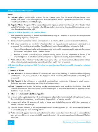
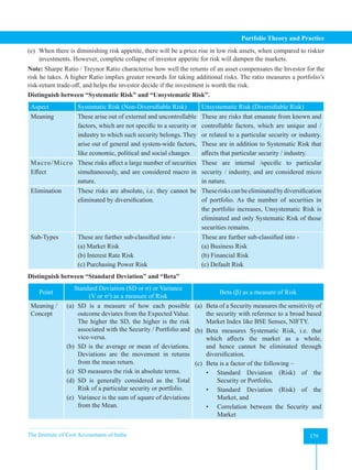
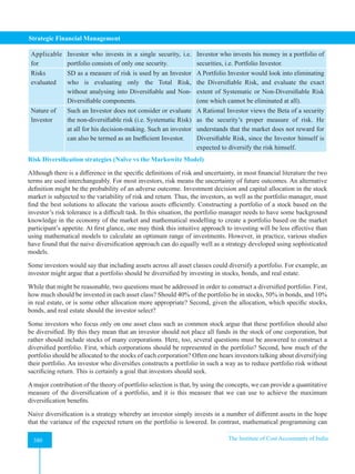
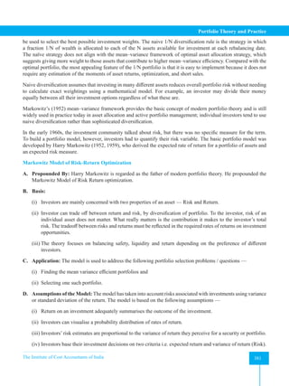
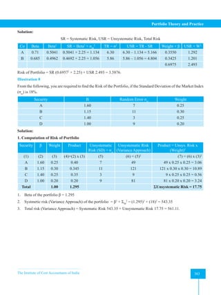
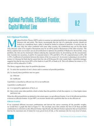
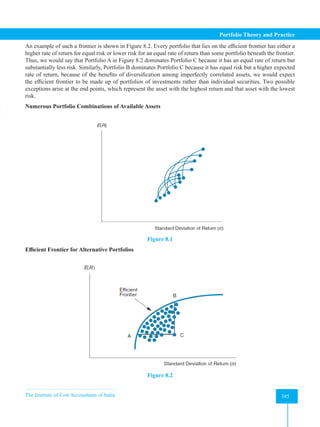
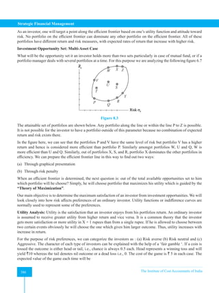
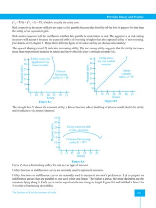
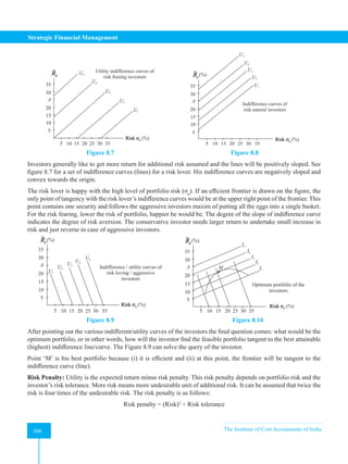
![The Institute of Cost Accountants of India 389
Portfolio Theory and Practice
Risk squared is the variance of return of the portfolio. Risk tolerance is a number from 0 to 100. High risk tolerance
means investor’s appetite to bear more risk for more return. Low tolerance is just reversed. Risk penalty decreases
as tolerance increases.
Example expected return from a portfolio is 16%, variance of return (risk squared) is 289% and the investor’s
tolerance is 60, the risk penalty will be = 289% ÷ 60 = 4.82%
Utility is = ERP
- Risk penalty = 16% - 4.82% = 11.18%
If the investor’s utility is minimum 10%, and since it exceeds 105, so the return from the portfolio will be accepted
by him.
Determination of Optimum Portfolio with inclusion of Risk Free Assets
So far, we have discussed the risk-return trade off only on risky asst i.e., determination of optimum portfolio of
risky assets. But when a risk free asset (rf
) is included with risky assets, what will be the optimum portfolio? And,
how funds will be allocated amongst different asset classes.
It’s a critical question as to how an investor will allocate his funds on two risky securities (say security A and
security B or stocks and bonds) and one risk free security with the help of capital allocation line. When optimizing
capital allocation, we want to work with the capital allocation line (CAL) offering the highest slope or Sharpe ratio.
The steeper the CAL, the greater is the expected return corresponding to any level of volatility. Now, we proceed
to asset allocation: constructing the risky portfolio of major asset classes, here a bond and a stock fund, with the
possible Sharpe ratio.
The asset allocation decision requires that we consider T-bills or another safe asset along with the risky asset
classes. The reason is that the Sharpe ratio we seek t maximize is defined as the risk premium in excess of the risk
free rate, divided by the standard deviation of the portfolio. We use T-bills as the risk free rate in evaluating the
Sharpe ratios of all possible portfolios. The portfolio that maximises the Sharpe ratio is the solution to the asset
allocation problem. Using only stocks, bonds, and bills is actually not so restrictive, as it includes all three major
asset classes.
To find out the optimum allocation of funds we require to find the Sharpe ratio and respective weights of risky
assets. The objective is to maximize the slope of the capital allocation line for any portfolio . thus, our objective
function is the slope or the Sharpe ratio or SP
.
SP
= [E(rp
) - rf
] ÷ σP
When we maximize the objective function, SP
, we have to satisfy the constraint that the weight of the portfolio’s
sum will be equal to 1 or (100%), i.e., W(Stock A + Stock B) = 1 or WA
+ WB
= 1
To optimize Max SP
= [E(rp
) - rf
] ÷ σP
, subject to ∑Wi
= 1. This is non-linear problem that can be solved using
standard tools of calculus.
In the case of the two risky assets, the solution for the weights of the optimal risky portfolio, P, is given by the
following equation:
WA
=
[E(RX
) - Rf
] × σy
2
- [E(RX
) - Rf
] × Covxy
[E(RX
) - Rf
]× σy
2
+ [E(Ry
) - Rf
] × σx
2
-[E(RX
) - Rf
+ E(Ry
) - Rf
]×Cov(xy)
In earlier chapters, we found the optimal complete portfolio given as optimal risky portfolio and the CAL generated
by a combination of this portfolio and T-bills. Now that we have constructed the optimal risky portfolio P, we
can use the individual investor’s degree of risk aversion, A, to calculate the optimal proportion of the complete
portfolio to invest in the risky component.](https://image.slidesharecdn.com/strategyfamous-230209132502-a14bc8e7/85/Strategy_Famous-pdf-401-320.jpg)
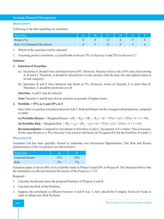
![The Institute of Cost Accountants of India 391
Portfolio Theory and Practice
Solution:
1. Basic Values of Factors for Portfolio Return Risk
Standard Deviation = σ Correlation Co-efficient = ρ Weights (W) Return = R
σA
= 3% ρAB = + 1 WA
+ 0.80 RA
= 12%
σB
= 7% WB
+ 0.20 RB
= 20%
Portfolio Return = Weighted Return = (WA
× RA
) + (WB
× RB
) = (12 × 80%) + (20 × 20%) = 9.6 + 4 = 13.6%
2. Risk of Portfolio [80% : 20% Ratio]
Risk (σAB
) = √ (σA
2
× WA
2
) + (σB
2
×WB
2
) + 2(σA
× WA
× σB
× WB
× ρAB
)
= √ (32
× 0.802
) + (72
× 0.202
) + (2 × 3 × 0.80 × 7 × 0.20 × 1)
= √ (5.76+1.96+6.72)
= √ 14.44
= 3.8%
3. Computation of Proportion of Investment in Security A and B if ρAB = -1
ρAB
= COVAB
/(σA
× σB
)
-1 = COVAB
/(3 × 7) Hence, COVAB
= -21
Proportion of Investment in Security A is computed as under –
WA
= (σB
2
- COVAB
)/(σA
2
+ σB
2
- 2COVAB
)
WA
= [72
- (-21)]/[32
+72
- 2 (-21)] = [(49+21)]/[9+49+42 ] = 70/100 = 0.70
So, Proportion of Investment in Security B, WB
= 1 – WA
= 1 - 0.70 = 0.30
Illustration 11
L Ltd and M Ltd has the following Risk and Return estimates:
RL
RM
σL
σM
Correlation co-efficient = rLM
20% 22% 18% 15% -1
Calculate the proportion of Investment in L Ltd and M Ltd to minimize the Risk of Portfolio.
Solution:
1. Basic Values of Factors for Determination of Portfolio Risk
Standard Deviation of L Ltd σL
18%
Standard Deviation of M Ltd σM
15%
Correlation co-efficient ρLM
-1
Weight of Security A WL
X
Weight of Security B WM
1 - X](https://image.slidesharecdn.com/strategyfamous-230209132502-a14bc8e7/85/Strategy_Famous-pdf-403-320.jpg)
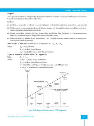
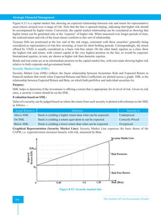
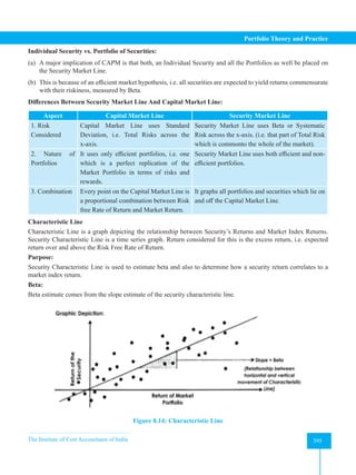
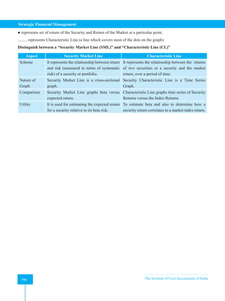
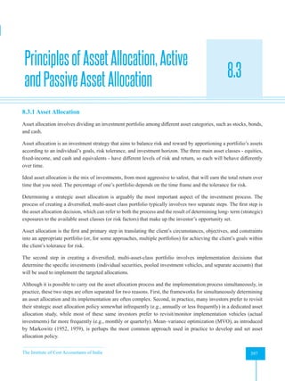
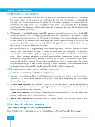
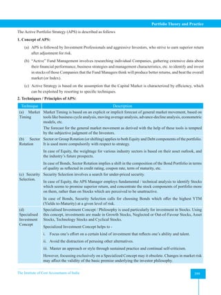
![The Institute of Cost Accountants of India 401
Portfolio Theory and Practice
2. Calculation of realized rate of return on Portfolio during 2017-2021
Stock P Stock Q Total
Year Proportion Return Net Return Proportion Return Net Return Net Return
1 2 3 4 = 3 × 2 5 6 7 = 5 × 6 8 = 4 + 7
2017 0.50 -12.24 -6.12 0.50 -7.00 -3.50 -9.62
2018 0.50 23.68 11.84 0.50 25.55 12.78 24.62
2019 0.50 34.44 17.22 0.50 44.09 22.05 39.27
2020 0.50 5.82 2.91 0.50 2.20 1.10 4.01
2021 0.50 28.30 14.15 0.50 20.16 10.08 24.23
40.00 42.51 82.51
Average rate of return = `82.51 ÷ 5 = 16.50%
2. Securities X and Y have standard deviations of 3% and 9%. Nitin is having a surplus of `20 Lakhs for
investment in these two securities. How much should he invest in each of these securities to minimize risk, if
the correlation coefficient for X and Y is: (a) -1; (b) -0.30; (c) 0; (d) 0.60
Solution:
1. Basic Values of Factors for Determination of Portfolio Risk
Standard Deviation of Security X σX
3%
Standard Deviation of Security Y σY
9%
Correlation co-efficient of Securities X and Y ρXY
-1,- 0.30, 0,0.60
Weight of Security X WX
a
Weight of Security Y WY
1-a
2. Computation of Investment in Securities
Proportion of Investment in Security X, WX
=
σY
2
- CovXY
σX
2
+ σY
2
- 2CovXY
Proportion of Investment in Security Y, WY
= 1 – WX
CovXY
= ρXY
× σX
× σY
If rXY
is CovXY
is Computation Investment
-1
-27
(-1×3×9)
→ WX
= [ σY
2
- CovXY
] ÷ [ σX
2
+ σY
2
- 2CovXY
] 0.750 in X
→ WX
= [92
- (-27)] ÷ [32
+ 92
- 2 × (-27)] 0.250 in Y
→ WX
= [81 + 27] ÷ [9 + 81 + 54] `15,00,000 in X
→ WX
= 108/144 = 0.75 `5,00,000 in Y
-0.3
-8.1
(-0.3×3×9)
→ WX
= [ σY
2
- CovXY
] ÷ [ σX
2
+ σY
2
- 2CovXY
] 0.839 in X
→ WX
= [92
- (-8.1)] ÷ [32
+ 92
- 2 × (-8.1)] 0.161 in Y
→ WX
= [81 + 8.1] ÷ [9 + 81 + 16.2] `16,78,000 in X
→ WX
= 89.1 / 106.2 = 0.839 `3,22,000 in Y](https://image.slidesharecdn.com/strategyfamous-230209132502-a14bc8e7/85/Strategy_Famous-pdf-413-320.jpg)
![Strategic Financial Management
402 The Institute of Cost Accountants of India
402
0
0
(0×3×9)
→ WX
= [ σY
2
- CovXY
] ÷ [ σX
2
+ σY
2
- 2CovXY
] 0.900 in X
→ WX
= [92
- 0] ÷ [32
+ 92
- 2 × 0] 0.100 in Y
→ WX
= [81 - 0] ÷ [9 + 81- 0] ` 18,00,000 in X
→ WX
= 81/90 = 0.90 ` 2,00,000 in Y
0.60
16.2
(0.6×3×9)
→ WX
= [ σY
2
- CovXY
] ÷ [ σX
2
+ σY
2
- 2CovXY
]
Reducing Risk below
3% is not possible.
→ WX
= [92
- 16.2] ÷ [32
+ 92
- 2 × 16.2]
→ WX
= [81 - 16.2] ÷ [9 + 81 – 32.4]
→ WX
= 64.8 / 57.60 = 1.125 1
At this correlation level, risk reduction is not possible.
3. An investor is considering two investment opportunities with the following risk and return characteristics.
Project P Q
Expected return 15% 22%
Risk 3% 7%
The investor plans to invest 80% of its available funds in share P and 20% in Q. the directors believe that the
correlation co-efficient between the returns of the shares is +1.0.
Required—
(a) Calculate the returns from the proposed portfolio of shares P and Q.
(b) Calculate the risk of the portfolio;
(c) Suppose the correlation coefficient between P and Q was -1. How should the company invest its funds in
order to obtain zero risk portfolio.
Solution:
1. Return of the Portfolio
Securities Expected return Proportion Return from portfolio
(1) (2) (3) (4) = (2)×(3)
P 15 0.8 12
Q 22 0.2 4.4
Return of the Portfolio 16.4
2. Basic Values of Factors for Determination of Portfolio Risk
Particulars Notation Value
Standard deviation of Security P σP
3%
Standard deviation of Security Q σQ
7%
Correlation co-efficient of Securities P and Q ρPQ
+ 1
Weight of Security P WP
0.80
Weight of Security Q WQ
0.20](https://image.slidesharecdn.com/strategyfamous-230209132502-a14bc8e7/85/Strategy_Famous-pdf-414-320.jpg)
![The Institute of Cost Accountants of India 403
Portfolio Theory and Practice
Risk of Portfolio i.e. Standard deviation of Portfolio of P and Q [80% : 20% Ratio]
σPQ = √ (σP
2
×WP
2
) + (σQ
2
×WQ
2
) + 2(σP
2
×WP
× σQ
×WQ
× σPQ
)
= √ (32
×0.802
) + (72
×0.202
) + (2× 3 × 0.80 × 7 × 0.20 × 1)
= √(9 × 0.64)+(49 × 0.04) + (6.72)
Risk = √5.76 + 1.96 + 6.72
= √14.44
= 3.8%
3. Computation of Investment in Security P and Q
Proportion of Investment in Security P, WP
=
σQ
2
- CovPQ
σP
2
+ σQ
2
- 2CovPQ
Proportion of Investment in Security Q, WQ
= 1 - WP
CovPQ
= ρPQ
× σP
× σQ
= -1 × 3 × 7 = -21
→WP
= [σQ
2
– CovPQ
] ÷ [σP
2
+ σQ
2
- 2CovPQ
]
→WP
= [72
– (-21)] ÷ [32
+72
-2 ×(-21)]
→WP
= [49 + 21] ÷ [9 + 49 + 42]
→WP
= 70 / 100
= 0.70
Proportion of Investment in Security Q, WQ
= 1 - WP
= 1 – 0.70 = 0.30
4. An investor has two portfolios known to be on minimum variance set for a population of three securities R, S
and T having the weights mentioned below:
WR
WS
WT
Portfolio X 0.30 0.40 0.30
Portfolio Y 0.20 0.50 0.30
It is supposed that there are no restrictions on short sales.
(a) What would be the weight for each stock for a portfolio constructed by investing `6,000 in Portfolio X and
`4,000 in Portfolio Y?
(b) Suppose the investor invests `5,000 out of `10,000 in Security R. How he will allocate the balance between
security S and T to ensure that his portfolio is on minimum variance set?
Solution:
1. Investment in Individual Securities
Security Portfolio X Portfolio Y Total Weight
R 6,000 × 0.30 = 1,800 4,000 × 0.20 = 800 2,600 2,600 ÷ 10,000 = 0.26
S 6,000 × 0.40 = 2,400 4,000 × 0.50 = 2,000 4,400 4,400 ÷ 10,000 = 0.44
T 6,000 × 0.30 = 1,800 4,000 × 0.30 = 1,200 3,000 3,000 ÷ 10,000 = 0.30
6,000 4,000 10,000 1.0000](https://image.slidesharecdn.com/strategyfamous-230209132502-a14bc8e7/85/Strategy_Famous-pdf-415-320.jpg)
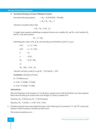
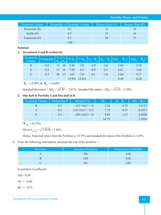
![Strategic Financial Management
406 The Institute of Cost Accountants of India
406
Solution:
1. Formula Approach (Alternative 1)
(a) Basic Values of Factors for Determination of Portfolio Risk
Standard Deviation of Security A σA
8%
Standard Deviation of Security B σB
12%
Standard Deviation of Security C σC
6%
Correlation co-efficient of Securities A and B 0.50
Correlation co-efficient of Securities A and C -0.40
Correlation co-efficient of Securities B and C 0.75
Weight of Security A WA
0.30
Weight of Security B WB
0.50
Weight of Security C WC
0.20
(b) Computation of Portfolio Risk (σABC
)
= √ (σA
2
×WA
2
)+(σB
2
×WB
2
)+(σC
2
×WC
2
)+2(σA
×WA
×σB
×WB
×ρAB
)+2(σA
×WA
×σC
×WC
×ρAC
)+2(σB
×WB
×σC
×WC
×ρBC
)
=√ (82
×0.32
)+(122
×0.52
)+(62
×0.22
)+(2×8×0.3×12×0.5×0.5)+(2×8×0.3×6×0.2×(-0.4))+(2×12×0.5×6×0.2×0.75)
= √ (64×0.09)+(144×0.25)+(36×0.04)+(14.4)+(-2.304)+(10.8)
= √ 5.76 + 36 + 1.44 + 14.4 - 2.304 + 10.8
= √ 66.096
= 8.13%
2. Matrix Approach (Alternative 2)
(a) Basic Values of Factors for Determination of Portfolio Risk
Variance of Security A σA
2
82
= 64
Variance of Security B σB
2
122
= 144
Variance of Security C σC
2
62
= 36
Covariance of Securities A and B [PAB
× σA
× σB
] COVAB
0.50 × 8 × 12 =48
Covariance of Securities A and C [PAC
× σA
× σC
] COVAC
- 0.40 × 8 × 6 = - 19.2
Covariance of Securities B and C [PBC
× σB
× σC
] COVBC
0.75 × 12 × 6 = 54
Weight of Security A WA
0.30
Weight of Security B WB
0.50
Weight of Security C WC
0.20](https://image.slidesharecdn.com/strategyfamous-230209132502-a14bc8e7/85/Strategy_Famous-pdf-418-320.jpg)
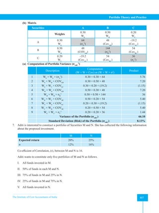
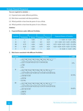
![The Institute of Cost Accountants of India 409
Portfolio Theory and Practice
IV
= √ (σM
2
×WM
2
)+(σN
2
×WN
2
)+2(σM
×WM
×σN
×WN
×ρMN
)
= √ (122
×0.252
)+(162
×0.752
)+(2×12×0.25×16×0.75×0.16)
= √ 9+144+11.52
= √164.52
= 12.38%
12.83%
V
= √ (σM
2
×WM
2
)+(σN
2
×WN
2
)+2(σM
×WM
×σN
×WN
×ρMN
)
= √ (122
×02
)+(162
×12
)+(2×12×0×16×1×0.16)
= √ 256
= 16%
16%
3. Best Portfolio from the point of view of risk:
The Best Portfolio from the point of view of risk is the one which has the least risk factor i.e., 10.42%.
Portfolio III [i.e., 75% of funds invested in M and 25% in N].
4. Best Portfolio from the point of return:
Portfolio V [i.e., 100% funds invested in the security, N] is the best from the point of return. This Portfolio
will earn a return of 25%.
8. AninvestorholdstwoequitysharesAandBinequalproportionwiththefollowingriskandreturncharacteristics:
e(RA
) 28%
σA
30%
e(RB
) 24%
σB
26%
The returns of these securities have a positive correlation of 0.7. You are required to calculate the portfolio
return and risk. Further, suppose that the investor wants to reduce the portfolio risk (σp
) to 17 per cent. How
much should the correlation coefficient be to bring the portfolio risk to the desired level?
Solution:
Basic Data
Notation Particulars Value
ρAB
Correlation co-efficient of Portfolio with market 0.7
σA
Standard Deviation of Share A 30%
σB
Standard Deviation of Share B 26%
σP
Risk of the Portfolio 17%
E(RA
) Return of the equity share A 28%
E(RB
) Return of the equity share B 24%](https://image.slidesharecdn.com/strategyfamous-230209132502-a14bc8e7/85/Strategy_Famous-pdf-421-320.jpg)
![Strategic Financial Management
410 The Institute of Cost Accountants of India
410
1. Computation of Expected Return
Expected Return [E(RP
)] = Proportion of A × E(RA
) + Proportion of B × E(RB
)
= 28(0.5) + 24(0.5)
= 14 + 12
= 26%
2. Computation of Portfolio Risk
σP = √ (σA
2
×WA
2
)+(σB
2
×WB
2
)+2(σA
×WA
×σB
×WB
×ρAB
)
= √ (302
×0.502
)+(262
×0.502
)+(2×30×0.50×26×0.50×0.70)
= √ 225+169+273
= √ 667
= 25.83%
3. Correlation Co - efficient
If the investor desires the portfolio standard deviation to be 17 per cent, the correlation coefficient will be
as computed below:
σP
= √ (σA
2
×WA
2
)+(σB
2
×WB
2
)+2(σA
×WA
×σB
×WB
×ρAB
)
= √ (302
×0.502
)+(262
×0.502
)+(2×30×0.50×26×0.50×CorAB
)
(17)2
= (30)2
(0.5)2
+ (26)2
(0.5)2
+2(0.5)(0.5)(30)(26) CorAB
289 = 225+169+390 CorAB
CorAB
= –105.25/390
= – 0.269
9. From the following information, ascertain the Market Price (X) of Risk of the portfolio -
Market Return
(Rm
)
Standard Deviation on
Market Return (σm
)
Return on Government
Bonds (Rf
)
Standard Deviation of the
Portfolio (σp
)
18% 6% 6% 8%
20% 8% 7% 4%
22% 9% 8% 12%
Also, determine the expected return for each of the above cases.
Solution:
1. Formulae for Expected Return and Market Price of Risk
Expected Return on Portfolio Rp
= Rf
+ λ × σP
Market Price of Risk of Portfolio λ = (Rm
− Rf
)/ σM](https://image.slidesharecdn.com/strategyfamous-230209132502-a14bc8e7/85/Strategy_Famous-pdf-422-320.jpg)
![The Institute of Cost Accountants of India 411
Portfolio Theory and Practice
2. Expected Return and Market Price of Risk
Market
Return
(Rm
)
Standard Deviation
on Market Return
(σm
)
Return on
Government
Bonds (Rf
)
Standard
Deviation of
Portfolio (σp
)
Market Price of
Risk (λ)
Expected Return
(RP
) = [Rf
+ λ × σP
]
(1) (2) (3) (4) (5)=[(1)-(3)]/(2) (6)=(3)+(5)×(4)
18% 6% 6% 8% 2
[(18-6)/6]
22%
[6% + 2 × 8%]
20% 8% 7% 4% 1.625
[(20-7)/8]
13.50%
[7% + 1.625 × 4%]
22% 9% 8% 12% 1.556
[(22-8)/9]
26.67%
[8% + 1.556 × 12%]
10. X Co. Ltd., invested on 1.4.2020 in certain equity shares as below:
Name of Co. No. of shares Cost (`)
D Ltd. 1,000 (` 10 each) 20,000
G Ltd. 500 (`1 each) 15,000
In September, 2020,10% dividend was paid out by D Ltd. and in October, 2020, 30% dividend paid out
by G Ltd. On 31.3.2021 market quotations showed a value of `22 and `29 per share for D Ltd. and G Ltd.
respectively.
On 1.4.2021, investment advisors indicate (a) that the dividends from D Ltd. and G Ltd. for the year ending
31.3.2022 are likely to be 20% and 35%, respectively and (b) that the probabilities of market quotations on
31.3.2022 are as given below:
Probability factor Price/ share of D Ltd. Price/ share of G Ltd.
0.2 22 29
0.5 25 31
0.3 28 33
You are required to—
(a) Calculate the average return from the portfolio for the year ended 31.3.2021
(b) Calculate the expected average return from the portfolio for the year 2021-22; and
(c) Advise X Co. Ltd., of the comparative risk in the two investments by calculating the standard deviation in
each case.
Solution:
1. Calculation of return on Portfolio for 2020-2021 (Calculation in `/ share)
Particulars D G
1. Market value by 31.03.21 22 29
2. Cost of investment 20 30
3. Gain / loss 2 (1)
4. Dividend received during the year Capital gain / loss by 31.03.21 1 0.3](https://image.slidesharecdn.com/strategyfamous-230209132502-a14bc8e7/85/Strategy_Famous-pdf-423-320.jpg)
![Strategic Financial Management
412 The Institute of Cost Accountants of India
412
5. Yield [(3) + (4)] 3 (0.7)
6. % return [(5) ÷ (2) ] × 100 15 (2.33)
7. Weight in the Portfolio [20 : 15] 57 43
Weighted average return = (57 × 15%) - (43 ×- 2.33%) = 7.55%
2. Calculation of Expected Return for 2021-22
Particulars D G
1. Expected dividend 2 0.35
2. Capital gain by 31.03.22
• (22 × 0.2) + (25 × 0.5) + (28 × 0.3)-22 = (25.3-22) 3.3
• (29 × 0.2) + (31 × 0.5) + (33 × 0.3)-29 = (31.2-29) 2.2
3. Yield[(1) + (2)] 5.3 2.55
4. Market value 01. 04.21 22 29
5. % return [(3) ÷ (4)] 24.09% 8.79%
6. Weight in Portfolio (1,000 × 22) : (500 × 29) 45 29
Weighted Average (Expected) Return = 13.38%
3. Standard deviation of D Ltd.
Expected Market
Value
Expected
Gain
Expected
Dividend
Expected
Yield
D
[(4) -5.3]
D2
Probability PD2
(1) (2) (3) (4) (5) (6) (7) (8)
22 0 2 2 -3.3 10.89 0.2 2.17
25 3 2 5 -0.3 0.09 0.5 0.05
28 6 2 8 2.7 7.29 0.3 2.19
4.41
Standard deviation = √PD2
= √ 4.41 = 2.1
4. Standard deviation of G Ltd.
Expected
Market Value
Expected
Gain
Expected
Dividend
Expected
Yield
D
[(4) -2.55]
D2
Probability PD2
(1) (2) (3) (4) (5) (6) (7) (8)
29 0 0.35 0.35 -2.2 4.84 0.2 0.97
31 2 0.35 2.35 -0.2 0.04 0.5 0.02
33 4 0.35 4.35 1.8 3.24 0.3 0.97
1.96
Standard deviation = √PD2
= √ 1.96 = 1.4
Share of company D Ltd. is more risky as the S.D. is more that of company G Ltd.](https://image.slidesharecdn.com/strategyfamous-230209132502-a14bc8e7/85/Strategy_Famous-pdf-424-320.jpg)
![The Institute of Cost Accountants of India 413
Portfolio Theory and Practice
11. The historical rates of return of two securities over the past ten years are given.
Calculate the Covariance and the Correlation coefficient of the two securities;
Years 1 2 3 4 5 6 7 8 9 10
Security A : (Return %) 12 8 7 14 16 15 18 20 16 22
Security B : (Return %) 20 22 24 18 15 20 24 25 24 18
Solution:
1. Computation of Factors
Year
Return of Deviation from Mean Variance of Covariance of
Security A
(R1
)
Security B
(R2
)
SA
(R1
- R 1
) (D1
)
SB
(R2
- R 2
) (D2
)
(D1
2
) (D2
2
)
R1
R2
[D1
× D2
]
(1) (2) (3) (4) (5) (6) (7) (8)
1 12 20 -2.8 -1 7.84 1 2.8
2 8 22 -6.8 1 46.24 1 -6.8
3 7 24 -7.8 3 60.84 9 -23.4
4 14 18 -0.8 -3 0.64 9 2.4
5 16 15 1.2 -6 1.44 36 -7.2
6 15 20 0.2 -1 0.04 1 -0.2
7 18 24 3.2 3 10.24 9 9.6
8 20 25 5.2 4 27.04 16 20.8
9 16 24 1.2 3 1.44 9 3.6
10 22 18 7.2 -3 51.84 9 -21.6
∑R1
= 148 ∑R2
= 210 207.6 100 -20
Security A Security B
Mean R 1
= ∑R1
÷ n
= 148 ÷ 10 = 14.8
R 2
= ∑R2
÷ n
= 210 ÷ 10 = 21
Variance σA
2
= ∑D1
2
÷ n = 207.6 / 10 = 20.76 σB
2
= ∑D2
2
÷ n = 100 / 10 = 10
Standard Deviation
σA
= √20.76 = 4.55 σB
= √10 = 3.162
2. Covariance and Correlation:
Combination Security A and B
Covariance CovAB
= Σ[D1
×D2
]÷ n = −20 ÷10 = −2
Correlation ρAB
= CovAB
/σA
× σB
= -2 / (4.55 × 3.162) = - 0.1390](https://image.slidesharecdn.com/strategyfamous-230209132502-a14bc8e7/85/Strategy_Famous-pdf-425-320.jpg)
![Strategic Financial Management
414 The Institute of Cost Accountants of India
414
12. The distribution of return of security “P” and the market portfolio “Q” is given below:
Probability
Return %
P Q
0.30 30 -10
0.40 20 20
0.30 0 35
You are required to calculate the expected return of security “P” and the market portfolio “Q”, the covariance
between the market portfolio and security and beta for the security,
Solution:
1. Expected Return and Risks of Security P
Scenario
Probability
(P)
Return
(R)%
Expected
Return %
Deviation (D)% D2 Variance
(P × D2
)
(1) (2) (3) (4) = (2) × (3) (5) = (3)-(2×4) (6) (7) = (2)×(6)
1 0.30 30 9 13 169 50.7
2 0.40 20 8 3 9 3.6
3 0.30 0 0 (17) 289 86.7
17.00% 141
Expected Return on Security P = 17.00%
Risk on Security (P) = σP
= √Variance = √141 = 11.87%
2. Expected Return and Risks of Market Portfolio Q
Scenario
Probability
(P)
Return (R)%
Expected
Return %
Deviation (D) % D2 Variance
(P × D2
)
(1) (2) (3) (4) = (2) × (3) (5) = (3)-∑(4) (6) (7) = (2)×(6)
1 0.30 (10) (3) (25.5) 650.25 195.075
2 0.40 20 8 4.5 20.25 8.1
3 0.30 35 10.5 (19.5) 380.25 114.07
15.50% 317.245
Expected Return on Market Portfolio Q = 15.50%
Risk on Security (Q) = σQ
= √Variance = √317.24 = 17.81%
3. Computation of Covariance of Securities P and Market Portfolio Q
Scenario
Probability
(P)
Deviation (DP
)
from Mean for P%
Deviation (DQ
) from
Mean for Q%
Deviation Product
(DPQ
) = DP
× DQ
Covariance
(P × DPQ
)
(1) (2) (3) (4) (5) = (3)×(4) (6) = (2)×(5)
1 0.30 13 (25.5) (331.5) (99.45)
2 0.40 3 4.5 13.5 5.4
3 0.30 (17) 19.5 (331.5) (99.45)
(193.5)
Covariance of Securities P and Market Portfolio Q [CovPQ
] = (193.5)
Beta = CovPQ
÷ σP
2
= -193.5 ÷ 317.245 = - 0.6099](https://image.slidesharecdn.com/strategyfamous-230209132502-a14bc8e7/85/Strategy_Famous-pdf-426-320.jpg)
![The Institute of Cost Accountants of India 415
Portfolio Theory and Practice
13. A Study by a Mutual Fund has revealed the following data in respect of the three securities:
Security σ (%) Correlation with Index, ρsm
P 20 0.66
Q 18 0.95
R 12 0.75
The Standard Deviation of the Market Portfolio (BSE Sensex) is observed to be 18%.
1. What is the sensitivity of returns of each stock with respect to the market?
2. What are the Co-variances among the various stocks?
3. What would be the risk of portfolio consisting of all the three stocks equally?
4. What is the beta of the portfolio consisting of equal investment in each stock?
5. What is the total systematic and unsystematic risk of the portfolio in (4)?
Solution:
1. Sensitivity
Security P Q R
Standard Deviation [A] 20.00 18.00 12.00
Correlation to Market Portfolio [B] 0.66 0.95 0.75
Beta (Sensitivity) = [A] × [B] / σM
[C] 0.73 0.95 0.50
2. Covariance between the securities
Covariance of Returns between the securities P and Q = CovPQ
= βP
× βQ
× σM
2
Securities P Q R
Beta 0.73 0.95 0.50
P 0.73 - 0.73 × 0.95× 324 0.73 × 0.50 × 324
Q 0.95 0.73 × 0.95× 324 - 0.50 × 0.95 × 324
R 0.50 0.73 × 0.50 × 324 0.50 × 0.95 × 324 -
Covariance Between Computation
P and Q βP
× βQ
× σ2
M
= 0.73 × 0.95 × 324 = 224.69
P and R βP
× βR
× σ2
M
= 0.73 × 0.50 × 324 = 118.26
Q and R βQ
× βR
× σ2
M
= 0.95 × 0.50 × 324 = 153.90
3. Risk of the Portfolio consisting of Equal Investment in each stock
Matrix
Securities P Q R
Weights 1/3
WP
1/3
WQ
1/3
WR
P
1/3
WP
400
(σP
2
)
224.69
(CovPQ
)
118.26
(CovPR
)
Q
1/3
WQ
224.69
(CovPQ
)
324
(σQ
2
)
153.90
(CovQR
)
R
1/3
WR
118.26
(CovPR
)
153.90
(CovQR
)
144
(σR
2
)](https://image.slidesharecdn.com/strategyfamous-230209132502-a14bc8e7/85/Strategy_Famous-pdf-427-320.jpg)
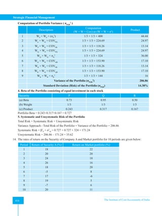
![The Institute of Cost Accountants of India 417
Portfolio Theory and Practice
(a) What is the beta of Security A?
(b) What is the characteristic line for security A?
Solution:
1. Computation of Beta of Security
Return of Deviation from Mean Variance of Covariance of
Period
Mkt.
(RM
)
A
(RA
)
Mkt.
(RM
− R M
)
(DM
)
A
(RA
− R A
)
(DA
)
Mkt.
(DM
2
)
A
(DA
2
)
RM
RA
[DM
× DA
]
(1) (2) (3)
(4)
[(2)-12]
(5)
[(3)-15]
(6)
(4)2
(7)
(5)2
(8)
(4)×(5)
1 22 18 10 3 100 9 30
2 20 20 8 5 64 25 40
3 18 24 6 9 36 81 54
4 16 26 4 11 16 121 44
5 20 18 8 3 64 9 24
6 8 -5 -4 -20 16 400 80
7 -6 17 -18 2 324 4 -36
8 5 19 -7 4 49 16 -28
9 6 -7 -6 -22 36 484 132
10 11 20 -1 5 1 25 -5
120 150 706 1174 335
Market Portfolio Shares of Company A
Mean R M
= ∑RM
÷ n
= 120 ÷ 10
=12
R A
= ∑RA
÷ n
= 150 ÷ 10
=15
Variance σM
2
= ∑DM
2
÷ n
= 706 ÷ 10
= 70.6
σA
2
= ∑DA
2
÷ n
= 1174 ÷ 10
= 117.4
Standard Deviation σM
= √70.6 = 8.40 σA
= √117.4 = 8.40
Covariance and Correlation:
Combination Market and A
Covariance CovMA
= [∑DM
× DA
] ÷ n
= 335 ÷ 10
= 33.5
Beta β β = CovMA
÷ σM
2
= 33.5 ÷ 70.6
= 0.4745](https://image.slidesharecdn.com/strategyfamous-230209132502-a14bc8e7/85/Strategy_Famous-pdf-429-320.jpg)
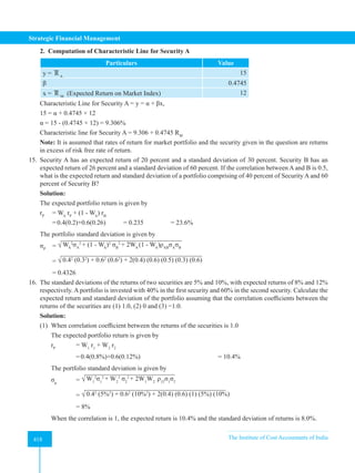
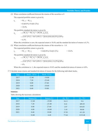
![Strategic Financial Management
420 The Institute of Cost Accountants of India
420
Mean return from stock X = ΣXi
/n = 32.80/5 = 6.56%
Mean return from stock Y = ΣYi
/n = -6.40/5 = -1.28%
σx2
= Σ(Xi
- X )2
/n-1 = 77.64/4 = 19.41
σy2
= Σ(Yi
- Y )2
/n-1 = 2135.48/4 = 533.87
Standard deviation of returns from stock X (σx
) = √19.41 = 4.41%
Standard deviation of returns from stock Y (σy
) = √533.87 = 23.11%
18. On the basis of the results from illustration 17, find out the portfolio return and portfolio risk assuming that
(i) weights are equal in both the stocks
(ii) weights are not given
Solution:
(i) Table showing the necessary calculations for covariance
Year (Xi
- X ) (Yi
- Y ) (Xi
- X )(Yi
- Y )
2017 5.84 -17.72 -103.48
2018 0.64 -22.12 -14.16
2019 1.44 28.88 41.59
2020 -1.76 -9.32 16.40
2021 -6.16 20.28 -124.92
-184.57
Wx
= 0.5 Wy
= 0.5
Covariance (x,y) = Σ(Xi
- X )(Yi
- Y ) / (n-1)
= -184.57/4
= - 46.14
Portfolio return (Rp
) = Wx
X + Wy
- Y
= 1/2×6.56 +1/2×(-1.28)
= 3.28-0.64
= 2.64%
Variance of return (σp
2
) = WX
2
σX
2
+ Wy
2
σy
2
+ 2WX
Wy
σXy
= (0.5)2
(19.41) + (0.5)2
(533.87) + [2×0.5×0.5×(-46.14)]
= 4.85 + 133.47 – 23.07
= 115.25
Portfolio risk (σp
) is given by the Standard Deviation of return = √115.25 = 10.74%
(ii) Correlation coefficient (ρxy
) = σxy
/ σx
σy
= - 46.14/ (4.41×23.11)
= -0.45](https://image.slidesharecdn.com/strategyfamous-230209132502-a14bc8e7/85/Strategy_Famous-pdf-432-320.jpg)
![The Institute of Cost Accountants of India 421
Portfolio Theory and Practice
Wx
= σy
2
– σx
σy
ρxy
/ (σx
2
+ σy
2
- 2σx
σy
ρxy
)
= (533.87-[4.41×23.11×(-0.45)])/(19.41+533.87-[2×4.41×23.11×(-0.45)])
= 0.90
Wy
= 1 – Wx
= 1 – 0.90
= 0.10
Rp
= Wx
X + Wy
Y
= 0.90×6.56 + 0.10×(-1.28)
= 5.904 – 0.128
= 5.78%
σp
2
= WX
2
σX
2
+ Wy
2
σy
2
+ 2WX
Wy
σXy
= (0.90)2
×19.41 + (0.10)2
×533.87 + 2×0.90×0.10×(-46.14)
= 15.72 + 5.3387 – 8.3052
= 12.7535
σp
= √12.7535
= 3.57%.
19. Illustration on Beta, Portfolio Variance, etc.
Following are the details of a portfolio consisting of three Shares:
Share Portfolio Weight Beta Expected Return % Total Variance
A 0.20 0.40 14 0.015
B 0.50 0.50 15 0.025
C 0.30 1.10 21 0.100
Standard Deviation of Market Portfolio Returns= 10%
You are given the following additional data: Covariance (A, B) = 0.030, Covariance (A, C) = 0.020,
Covariance (B, C) = 0.040
Calculate the following: (i) The Portfolio Beta, (ii) Residual Variance of each of the three Share, (iii) Portfolio
Variance using Sharpe Index Model, (iv) Portfolio Variance (on the basis of Modern Portfolio Theory given
by Markowitz).
Solution:
1. Determination of Portfolio Beta
Share Name Portfolio Weight Beta Weighted Beta
A 0.20 0.40 0.08
B 0.50 0.50 0.25
C 0.30 1.10 0.33
Portfolio Beta 0.66](https://image.slidesharecdn.com/strategyfamous-230209132502-a14bc8e7/85/Strategy_Famous-pdf-433-320.jpg)
![The Institute of Cost Accountants of India 423
Portfolio Theory and Practice
The Standard Deviation of the Market Portfolio (BSE Sensex) is observed to be 15%
1. What is the Sensitivity of Returns of each Stock with respect to the Market?
2. What are the Co-Variances among the various Stocks?
3. What would be the Risk of Portfolio consisting of all the three Stocks equally?
4. What is the Beta of Portfolio consisting of equal Investment in each Stock?
5. What is the total Systematic and Unsystematic Risk of the Portfolio in (4)?
Solution:
1. Sensitivity
Security A B C
Standard Deviation (σ) 20.00 18.00 12.00
Correlation to Market Portfolio (ρsm
) 0.66 0.95 0.75
Beta (Sensitivity) = ρSM
× (σ security)/(σ market) 0.88 1.14 0.60
2. Covariance between the securities
Covariance of Returns between the two securities = Covs1,s2
= βs1
× βs2
× σM
2
CovAB
= βA
× βB
× σM
2
CovAC
= βA
x βB
x σM
2
CovBC
= βB
× βC
× σM
2
0.88 × 1.14 × 225 = 225.72 0.88 × 0.60 × 225 = 118.80 1.14 × 0.60 × 225 = 153.90
3. Risk of the Portfolio consisting of Equal Investment in each stock
Securities A B C
Weights WA
= 1/3 WB
= 1/3 WC
= 1/3
A WA
= 1/3 σA
2
= 400 Cov(A,B) = 225.72 Cov(A,C) = 118.80
B WB
= 1/3 Cov(A,B) = 225.72 σB
2
= 324 Cov(B,C) = 153.90
C WC
= 1/3 Cov(A,C) = 118.80 Cov(B,C) = 153.90 σC
2
= 144
A B C
A
WA
× WA
× σA
2
1/3 × 1/3 × 400 = 44.44
WA
× WB
× CovAB
1/3 × 1/3 × 225.72 = 25.08
WA
× WC
× CovAC
1/3 × 1/3 × 118.80 = 13.20
B
WA
× WB
× CovAB
1/3 × 1/3 × 225.72 = 25.08
WB
× WB
× σB
2
1/3 × 1/3 × 324 = 36.00
WB
× WC
× CovBC
1/3 × 1/3 × 153.90 = 17.10
C
WA
× WC
× CovAC
1/3 × 1/3 × 118.80 = 13.20
WB
× WC
× CovBC
1/3 × 1/3 × 153.90 = 17.10
WC
× WC
× σC
2
1/3 × 1/3 × 144 = 16.00
Variance of the Portfolio (σABC
2
) 207.20
Standard Deviation (Risk) of the Portfolio (σABC
) 14.3944
4. Beta of the Portfolio consisting of equal Investment in each Stock = (0.88+1.14+0.60)/3 = 0.873
5. Systematic and Unsystematic Risk of the Portfolio [Variance Approach]](https://image.slidesharecdn.com/strategyfamous-230209132502-a14bc8e7/85/Strategy_Famous-pdf-435-320.jpg)
![Strategic Financial Management
424 The Institute of Cost Accountants of India
424
Total Risk = 207.20
Systematic Risk
Βp
2
× σM
2
= (0.0873)2
× 225 = 171.48
Unsystematic Risk (Balancing figure)
207.20 – 171.48 = 35.72
21. Illustration on Capital Market Line – Measuring Expected Return
Portfolio A, a fully diversified Portfolio, has a Standard Deviation of 6%. The NIFTY has yields a Return of
16.5%, with a Standard Deviation of 4%, Ascertain the expected Return of Portfolio A under the following
three cases –
1. 5.80% ` 100 Central Government guaranteed RBI Bonds is traded at ` 116,
2. Market’s Attitude towards risk is 3,
3. Risk Free Return is 7%.
Solution:
Expected Return on Portfolio Rp
= Rf
+ (λ x σp
) Where, λ = (Rm
- Rf
)/σm
Particulars Case 1 Case 2 Case 3
Risk Free Return [RF
] Return/(Market Price )
= (100 × 5.8%)/116
= 5%
4.5%
[Note]
7%
[Given]
Market’s Attitude towards
Risk (λ) = (Rm
-Rf
)/σm
(16.50% - 5%)/(4%)
= 2.875
3
[Given]
(16.50% - 7%)/(4%)
= 2.375
Expected Return [Rp
]
= Rf
+ (λ × σp
)
5% + (2.875 × 6%)
= 22.25%
4.5% + (3 × 6%)
= 22.50%
7% + (3 × 6%)
= 25%
Note: Risk Free Return [Case 2]: (Rm
- Rf
)/σm
= 3 → (16.5 - Rf
)/(4%) = 3 → Rf
= 16.5 – 12% = 4.50%
22. Illustration on Capital Market Line (CML) – Market Price of Risk
From the following information, as certain the Market Price of Risk of the portfolio –
Market Return (Rm
) Standard Deviation on
Market Return (σm
)
Return on Government
Bonds (Rf
)
Standard Deviation of the
Portfolio (σρ
)
18% 6% 6% 8%
20% 8% 7% 4%
22% 9% 8% 12%
Also, determine the expected return for each of the above cases
Solution:
1. Formulae for Expected Return and Market Price of Risk
Expected Return on Portfolio Rp
= Rf
+ ( λ × σp
)
Market Price of Risk of Portfolio λ = (Rm
- Rf
)/σm](https://image.slidesharecdn.com/strategyfamous-230209132502-a14bc8e7/85/Strategy_Famous-pdf-436-320.jpg)
![The Institute of Cost Accountants of India 425
Portfolio Theory and Practice
2. Expected Return and Market Price of Risk
Market
Return
Rm
SD on
Market
Return (σm
)
Return on
Govt Bonds
(Rf
)
SD of
Portfolio
(σρ
)
Market Price of Risk
(λ) = [(Rm
- Rf
)/σm
]
Expected Return
(Rp
) = [Rf
+ λ × σρ
]
(1) (2) (3) (4) (5) = [(1) – (3) / (2)] (6) = (3) + (5) × (4)
18% 6% 6% 8% (18-6)/6 = 2 [6% + 2 × 8%] = 22%
20% 8% 7% 4% (20-7)/8 = 1.625 [7%+1.625×4%]=13.50%
22% 9% 8% 12% (22-8)/9 = 1.556 [8%+1.556×12%]= 26.67%
23. A Stock costing `120 pays no dividends. The possible prices that the Stock might sell for at the end of the year
with the respective probabilities are given below. Compute the Expected Return and its Standard Deviation.
Price 115 120 125 130 135 140
Probability 0.1 0.1 0.2 0.3 0.2 0.1
Solution:
Price Return (R) = P – `120 Probability (P) Expected Return (P × R) D = R - R D2
P × D2
115 (5) 0.1 (0.5) (13.5) 182.25 18.225
120 0 0.1 0.0 (8.5) 72.25 7.225
125 5 0.2 1.0 (3.5) 12.25 2.450
130 10 0.3 3.0 1.5 2.25 0.675
135 15 0.2 3.0 6.5 42.25 8.450
140 20 0.1 2.0 11.5 132.25 13.225
Total R = 8.5 50.250
Expected Return on Security = `8.5, Risk of Security = σ = √Variance = √50.25 = `7.09
OR (`7.09 ÷ `120) = 5.91%
24. From the following data pertaining to returns of Shares of Companies A, B Market for the past 5 years, find
Beta (β) of A B –
Year 1 2 3 4 5
Market 12% 14% 13% 12% 14%
Company A 16% 8% 13% 14% 19%
Company B 14% 17% 15% 20% 19%
Solution:
1. Computation of Factors
Year RM
RA
RB DM
= RM
- R M
DA
= RA
- R A
DB
= RB
- R B
DM
2
DM
× DA
DM
× DB
(1) (2) (3) (4) (5) = (2) – 13 (6) = (3)-14 (7) = (4)-17 (8) = (5)2
(9)= (5)×(6) (10)=(5)×(7)
1 12 16 14 -1 2 -3 1 -2 3
2 14 8 17 1 -6 0 1 -6 0](https://image.slidesharecdn.com/strategyfamous-230209132502-a14bc8e7/85/Strategy_Famous-pdf-437-320.jpg)
![Strategic Financial Management
426 The Institute of Cost Accountants of India
426
3 13 13 15 0 -1 -2 0 0 0
4 12 14 20 -1 0 3 1 0 -3
5 14 19 19 1 5 2 1 5 2
65 70 85 4 -3 2
2. Computation of Beta
Market Portfolio Shares of Company A Shares of Company B
Mean R M
=∑RM
÷n=65÷5=13 R A
=∑RA
÷n=70÷5=14 R M
= ∑RB
÷ n = 85÷5
=17
Variance
Covariance
σM
2
=∑DM
2
÷ n=4÷5=0.80 CovMA
=∑[DM
× DA
]=3÷5= -0.60 CovMB
= ∑[DM
× DB
] = 2 ÷ 5
= 0.40
Beta CovMA
÷ σM
2
= -0.60 ÷ 0.80 =
-0.75
CovMB
÷ σM
2
= 0.40 ÷ 0.80
= 0.50
25. Shiva Ltd invested at the beginning of Year 1 in certain Equity Shares as below
Name of the Company No. of shares Cost (`)
M Ltd 1,000 (`100 each) 2,00,000
N Ltd 500 (`10 each) 1,50,000
In Year 1, 10% Dividend was paid out by M Ltd, and 30% Dividend paid out by N Ltd. At the end of year 1,
market quotations showed a value of `220 and `290 per Share for M Ltd and N Ltd respectively.
At the beginning of year 2, Investment Advisors indicate – (a) that the Dividends from M Ltd and N Ltd for
the Year 2 are likely to be 20% and 35% respectively, and (b) that the probabilities of market quotations at the
end of Year 2 are as below:
Probability Price per Share of M Ltd Price per Share of N Ltd
0.2 220 290
0.5 250 310
0.3 280 330
1. Calculate the Average Return from the Portfolio for the Year 1.
2. Calculate the Expected Average Return from the Portfolio for the Year 2, and
3. Advise Shiva Ltd of the comparative risk in the two Investments by calculating the Standard Deviation in
each case.
Solution:
1. Calculation of closing MPS and total Return for 2018-2019
EMPS = Expected Market Price per Share, Gain = Closing MPS Less Opening MPS, Div. = Dividend,
Yield = Div. + Gain
M Ltd. N Ltd.
Prob. Clg. Opg. Gain Div. Yield MPS ×
Prob.
Clg. Opg. Gain Div. Yield MPS ×
Prob.
0.2 220 220 0 20 20 44 290 290 0 3.5 3.5 58](https://image.slidesharecdn.com/strategyfamous-230209132502-a14bc8e7/85/Strategy_Famous-pdf-438-320.jpg)
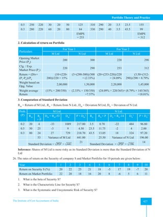
![Strategic Financial Management
428 The Institute of Cost Accountants of India
428
Solution:
1. Computation of Beta of Security
Period RM
RS DM
= (RM
- R M
) DS
= (RS
- R S
) DM
2
DS
2
DM
× DS
(1) (2) (3) (4)=[(2)-12] (5)=[(3)-15] (6) = (4)2
(7)=(5)2
(8)=(4)×(5)
1 22 20 10 5 100 25 50
2 20 22 8 7 64 49 56
3 18 25 6 10 36 100 60
4 16 21 4 6 16 36 24
5 20 18 8 3 64 9 24
6 8 -5 -4 -20 16 400 80
7 -6 17 -18 2 324 4 -36
8 5 19 -7 4 49 16 -28
9 6 -7 -6 -22 36 484 132
10 11 20 -1 5 1 25 -5
120 150 706 1148 357
Market Portfolio Security of Company S
Mean R M
= ∑RM
÷ n = 120÷10=12 R S
=∑RS
÷ n = 150÷10=15
Variance σM
2
=∑DM
2
÷ n = 706 ÷ 10 = 70.6 σS
2
=∑DS
2
÷ n = 1148 ÷ 10 = 114.8
Standard Deviation σM
= √70.60 = 8.40 σS
= √114.80 =10.71
Covariance and Correlation:
Combination Market and S
Covariance CovMS
= ∑[DM
× DS
] ÷ n = 357 ÷ 10 = 35.7
Beta βS
BS
= CovMS
/σM
2
= 35.7/70.6 = 0.51
2. Computation of Characteristic Line for Security S
Particulars Value
y = R A
15
β 0.51
x = R M
(Expected Return on Market Index) 12
Characteristic Line for Security S = y = α + βx, α = 15 – (0.51 × 12) = 8.88%
15 = α + (0.51 × 12)
Characteristic line for Security S = 8.88 + 0.51 RM
Note: It is assumed that Rates of Return for Market Portfolio and the Security given in the question is returns
in excess of Risk Free Rate of Return.](https://image.slidesharecdn.com/strategyfamous-230209132502-a14bc8e7/85/Strategy_Famous-pdf-440-320.jpg)
![The Institute of Cost Accountants of India 429
Portfolio Theory and Practice
3. Analysis of Risk into Systematic Risk and Unsystematic Risk
Particulars Standard Deviation Approach Variance Approach
Total Risk 10.71% 114.80%
Systematic Risk β × σm
= 0.51 × 8.40 = 4.284% β2
× σm
2
= 0.512
× 70.60 =
18.363%
Unsystematic Risk [Total Risk -
Systematic Risk]
10.71 - 4.284 = 6.426% = 114.80 - 18.363 = 96.437%
27. Illustration on Systematic Unsystematic Risk
The following are the Returns of Share S and the Market (M) for the Last 6 years –
Year 1 2 3 4 5 6
Return on S (%) 18 9 20 -10 5 12
Return on Market Portfolio 15 7 16 -13 4 7
1. Calculation the Covariance Correlation Co-efficient of returns
2. Determine the Beta co-efficient for S
3. What is S’s Total Risk?
4. How much is the Systematic Risk?
Solution:
1. Computation of Covariance and Correlation Co-efficient
Years RM
RS DM
= (RM
- R M
) DS
= (RS
- R S
) DM
2
DS
2
DM
x DS
(1) (2) (3) (4)=[(2)-6] (5)=[(3)-9] (6)=(4)2
(7)=(5)2
(8)=(4)×(5)
1 15 18 9 9 81 81 81
2 7 9 1 0 1 0 0
3 16 20 10 11 100 121 110
4 -13 -10 -19 -19 361 361 361
5 4 5 -2 -4 4 16 8
6 7 12 1 3 1 9 3
36 54 0 0 548 588 563
Market Portfolio Shares of S
Mean R M
= ∑RM
÷ n = 36 ÷ 6 = 6 R S
=∑RS
÷ n = 54 ÷ 6 = 9
Variance σM
2
=∑DM
2
÷ n = 548 ÷ 6 = 91.33 σS
2
=∑DS
2
÷ n = 588 ÷ 6 = 98
Standard Deviation
σM
= √ 91.33 = 9.56 σS
= √98 = 9.90](https://image.slidesharecdn.com/strategyfamous-230209132502-a14bc8e7/85/Strategy_Famous-pdf-441-320.jpg)
![Strategic Financial Management
430 The Institute of Cost Accountants of India
430
2. Computation of Covariance Corelation
Combination Market and S Combination Market and S
Covariance CovMS
= ∑[DM
× DS
] ÷ n
= 563 ÷ 6
= 93.83
Corelation ρMS
= CovMS
/σM
× σS
= 93.83/(9.56 × 9.90)
= 0.99
3 Computation of Beta: Beta of Security = βS
= COVMS
/(σM
2
) = 93.83/91.33 = 1.03
4. Computation of Systematic and Unsystematic Risk
Particulars Standard Deviation Approach Variance Approach
Total Risk 9.90 98%
Systematic Risk β × σM
= 1.03 × 9.56 = 9.847% β2
× σM
2
= 1.032
× 9.562
= 9.847
=1.061 × 91.39 = 96.96%
Unsystematic Risk = Total Risk Less
Systematic Risk
9.90% - 9.847% = 0.053% 98% - 96.96% = 1.04%
Solved Case Studies
1. Case Study on Modifying Portfolio Beta
A Portfolio Manager has the following four stocks in his portfolio:
Security No. of Shares Market Price Per Share (`) β
A 10,000 50 0.9
B 5,000 20 1.0
C 8,000 25 1.5
D 2,000 200 1.2
1. Compute the Portfolio Beta.
2. If the Portfolio Manager seeks to reduce the Beta to 0.8, how much Risk Free Investment should he bring
in?
3. If the Portfolio Manager seeks to increase the Beta to 1.2, how much Risk Free Investment should he bring
in?
Solution:
1. Computation of Portfolio Beta
Security No of Shares MP (`) Market Value of Investments Beta Beta = Market Value × Beta
A 10,000 50 5,00,000 0.9 4,50,000
B 5,000 20 1,00,000 1.0 1,00,000
C 8,000 25 2,00,000 1.5 3,00,000
D 2,000 200 4,00,000 1.2 4,80,000
12,00,000 13,30,000
Therefore, Portfolio Beta = Product/(Market Value) = 13,30,000/12,00,000 = 1.108](https://image.slidesharecdn.com/strategyfamous-230209132502-a14bc8e7/85/Strategy_Famous-pdf-442-320.jpg)
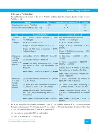
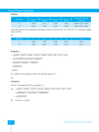
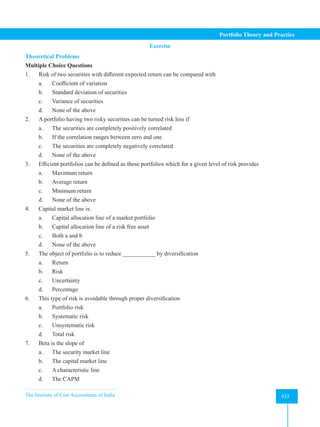


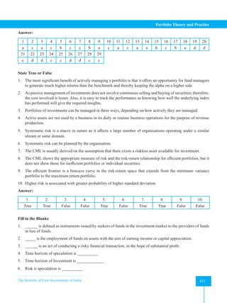


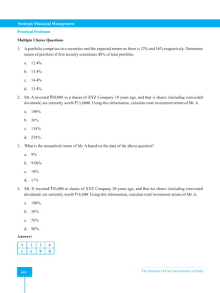
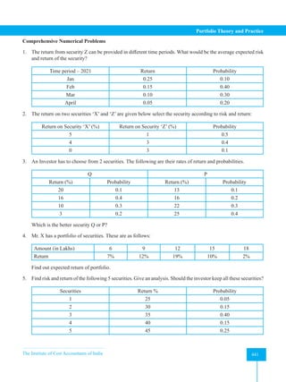
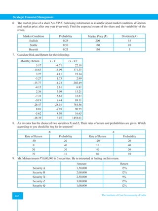
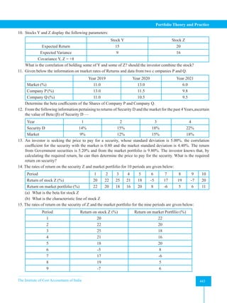
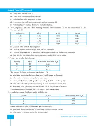
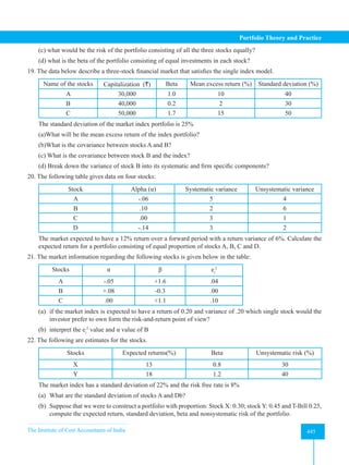
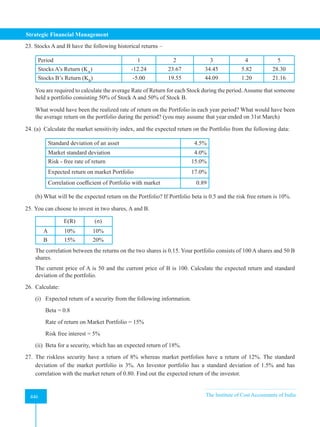
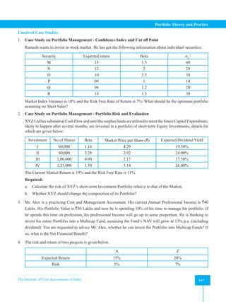
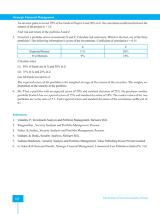

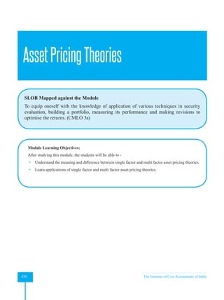
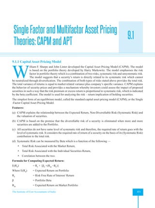
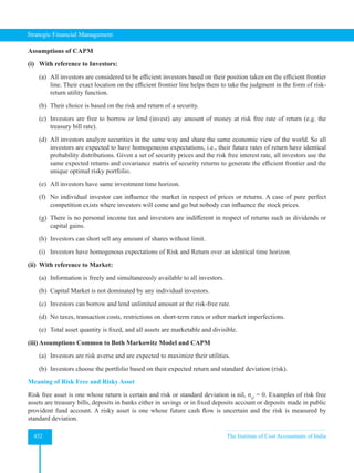
![The Institute of Cost Accountants of India 453
Asset Pricing Theories
Covariance of a Risky Asset with Risk Free Asset
Let us consider x as risk free security and y as risky security.
Covxy
= Ʃ
n
i=1
[Rx
- E(Rx
)][Ry
- E(Ry
)]/N
where Rx
– E(Rx
) will be zero because return is certain. Hence the value of covariance will also be zero.
Similarly, r =
Covxy
σx
σy
will also be zero.
Combining a Risk Free Asset with a Risky Asset
Now let us see what happens to Markowitz efficient frontier line which earlier had only risky assets, now risk free
asset is included. What will be the expected return and risk of the portfolio after inclusion of the risk free asset?
The expected return of the portfolio will be –
ERP
= W1
f1
+ (1-W1
)E(Rx
)
where W1
=Proportion of investment in risk free assets only, (1-W1
) = Balance of proportion invested in risky asset,
f1
=Rate of return in risk free asset only, E(Rx
)=Expected return on risky security x, ERP
=Expected return of the
portfolio.
We know portfolio risk = W1
2
σ2
f
+ W2
2
σ2
x
+ 2rW1
W2
σf
σx
[W2
= Proportion of investment in risky securities, W1
=
Proportion of investment in risk free securities, σf
= Standard deviation of risk free security, σx
= Standard deviation
of risky security.]
Where σf
= standard deviation of risk free security is zero (r) or correlation coefficient is also zero. What remains
is the risk of the risky asset only, i.e., W2
2
σ2
x
Illustration 1
Risk free return on a 91-day treasury bill is 6.00% p.a. Return on risky security is 12% and the standard deviation is
9.0%. Find out the risk and return of the portfolio. It is assumed that the investor invests equally in two securities.
Solution:
E(RP
) = 0.50 × 6.00 × + 0.50 × 12 = 3.00 + 6.00 = 9.00%
σp
= 0.50 × 0 + (0.50)2
× (9.0)2
= 4.50%
An investor is free to invest all his wealth in a risk free asset or he can invest all his wealth in risky asset. He can
also borrow at risk free rate and invest in risky asset so as to enhance his return. Under different combinations of
lending and borrowing of risky and risk free securities at the risk free rate of interest the expected return and risk
of the portfolio will be as under:](https://image.slidesharecdn.com/strategyfamous-230209132502-a14bc8e7/85/Strategy_Famous-pdf-465-320.jpg)
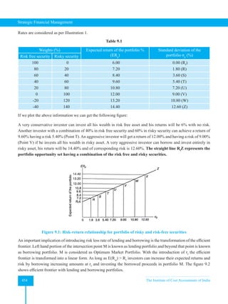
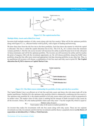
![The Institute of Cost Accountants of India 457
Asset Pricing Theories
Capital Market Line (CML)
With the ability to borrow and lend at the risk free rate of interest (rf
) with an investment in market portfolio M, the
old efficient portfolio has transformed into a new efficient portfolio emanating from Rf
through market portfolio M.
This new linear efficient frontier is known as Capital market Line or simply CML. All portfolios lying along the
capital market line will dominate all other portfolios in respect of risk and returns. Therefore, all efficient portfolios
are lying on the capital market line. All inefficient portfolios are lying below the capital market line.
The CML not only represents the new efficient frontier, but also expresses the equilibrium pricing relationship
between expected return E(R) and risk (σ) for all efficient portfolios lying along the CML. Since the equation for
any line is expressed as y = a + bx, where a represents the vertical intercept and b represents the slope of line, the
pricing relationship of CML can be easily determined as: a = rf
and b = [E(Rm
) – Rf
]/σm
Thus, the CML relationship for any efficient portfolio can be expressed with the help of an equation as:
E(Ri
) = rf
+ {[E(Rm
) – Rf
]/σm
} σi
The above equation for efficient portfolio have two parts (a) the risk free rate of return (Rf
) and (b) a risk premium
{[E(Rm
) – Rf
]/σm
} σi,
that is proportionalto portfolios risk (σi
).
The slope of the CML (E(Rm
) – Rf
)/σm
is called the market price of risk and this component will be same for all the
portfolios lying on the CML. The most interesting part to note, the factor that distinguishes the expected returns
amongst CML portfolios, is the magnitude of risk (σi
). The greater the risk (σi
), the greater is the risk premium and
the expected return on the portfolio.
Illustration 3
Assume that expected return om market portfolio = 18% with a standard deviation of 20% . If the = 6%, the slope
of the CML would be?
Solution:
(E(RM
) –Rf
)/σm
= (18 – 6)/20 = 12/20 = 0.60
The slope of the CML shows the equilibrium price of risk in the market. In our above example, a risk premium
of 0.60 indicates that the market demands this amount of return for each percentage increase in the portfolio risk.
Therefore, the CML equation is: ERi
= 0.06 + 0.60σi
Now, the CML’s intercept would be 6% (rf
).
Expected return will change for changes in the different magnitudes of risk of individual security. It is important to
recognize that the CML pricing holds only for efficient portfolio that lies along its line. All individual securities and
inefficient portfolios will lie below the line. It not only represents the efficient portfolio lying along its line but also
represents zero unsystematic risk of portfolios. The total risk (σi
) is the sum of systematic and unsystematic risk.
In a well diversified efficient portfolio, their risk, can be thought of either total risk or systematic risk only.
Thus, CML explains that price for appropriate measures of risk is only systematic risk included in the portfolio.
Illustration 4
Consider Illustration 3 and additionally assume that the ratio of investment is 1/3 and 2/3 respectively for risk free
and risky securities. Find out the expected return and risk of the portfolio.](https://image.slidesharecdn.com/strategyfamous-230209132502-a14bc8e7/85/Strategy_Famous-pdf-469-320.jpg)
![Strategic Financial Management
458 The Institute of Cost Accountants of India
Solution:
Given: ERm
18% ; Rf
= 6%; σm
= 20%; proportion of market portfolio = 2/3rd
and proportion of risk free asset (rf
)
= 1/3rd
E(Rp
) = (1/3) × 6 + (2/3) ×18 = 14%
Risk of the portfolio σp
= [W1
2
σ1
2
+ W2
2
σ2
2
+2×r×σ1
×σ2
×W1
×W2
]1/2
Where W1
= rf
, W2
= Risky portfolio, σp
= risk of the risk free security, σp
= risk of the risky asset.
σp
= 2/3 × 20 = 13.33% (risk of market portfolio only). [r is nil].
E(Rp) based on CML = Rf + }
}E(Rm
) - Rf
σM
[
[ σp
= 6 +
18 - 6
20 [
[ × 13.33
= 6 + 8 = 14% (Same as above)
The Capital Asset Pricing Model: CML establishes the equilibrium relationship between expected return and risk
of efficient portfolios only having no unsystematic risk. Two important questions arise:
(a) What will be the risk-return characteristics of all securities and portfolios whether efficient or inefficient?
(b) What will be the equilibrium relationship that should exist between the expected return of a security and its
relevant risk?
Under CAPM, risk of an individual security is directly related to the volatility of the returns of market portfolio.
Risk of an individual security is only the systematic risk. Systematic risk is measured as the covariance of an
individual risky security with the market portfolio. The greater the covariance, the greater the required return.
AS already stated, all investors hold the same market portfolio M, the required return should be a function of the
covariance between the security return and the market portfolio. The equilibrium relationship between securities
expected returns and their covariance’s with the market portfolio is called the Security Market Line (SML)
which is commonly referred to as CAPM.
Figure 9.5: The capital asset pricing model
The covariance of any asset with itself is represented by its variance, i.e., Covi,i
= σ2
i
. The return on market portfolio
should depend on its own risk, which is given by the variance of the market-return σMM
(σ2
M
). Therefore, the risk-
return relationship is shown as:](https://image.slidesharecdn.com/strategyfamous-230209132502-a14bc8e7/85/Strategy_Famous-pdf-470-320.jpg)
![The Institute of Cost Accountants of India 459
Asset Pricing Theories
E(Ri
) = Rf
+
E(Rm
)-Rf
σ2
m
[
[ (Covi,m
)
E(Ri
) = Rf
+ [E(Rm
) - Rf
] ×σi
× σm
× ρim
σm
× σm
Rf
+ [E(Rm
) - Rf
] ×
σi
σm
× ρim
The term Covim
/σ2
m
is known as security’s beta which reflects the security’s systematic risk with respect to market
return.
The above equation has two components (1) Risk free rate of return rf
and (2) Market risk premium
E(Rm
)-Rf
σ2
m
[
[
Covi,m
which is proportional to the covariance of the security’s rate of return with respect to the market return. The
slope of the CAPM is given by E(Rm
) - Rf
/ σ2
m
and is same for all securities. The magnitude of Covim
determines
how much additional return an investor should get above the risk free rate (Rf
) to compensate for additional
risk undertaken by him. This risk belongs to only systematic risk as unsystematic risk has totally been
diversified.
The CAPM relationship can be expressed in term of security’s beta (β)
We know that (β) =
Cov(i,m)
σ2
m
Substituting this value in equation E(Ri
) = Rf
+
E(Rm
)-Rf
σ2
m
[
[ (Covi,m
) we get
E(Ri
)=Rf
+ [E(Rm
) – Rf
]βi
Security Market Line (SML)
We can plot the required rate of returns Rj
and systematic risk (β) as expressed in CAPM to produce a graph of the
SML as shown below:
Since all securities are expected to plot along the SML, the direct and convenient way to determine the expected
return provided we know the beta of the security.
SMLclassifies the securities based on the value of beta. If the value of β is less than one, it reflects the security
as conservative or defensive while if β exceeds one, it reflects the security as aggressive one.
Figure 9.6: Security market line
One of the major assumptions of the CAPM is that the market is in equilibrium and the expected rate of return](https://image.slidesharecdn.com/strategyfamous-230209132502-a14bc8e7/85/Strategy_Famous-pdf-471-320.jpg)
![Strategic Financial Management
460 The Institute of Cost Accountants of India
is equal to the required rate of return for a given level of market risk or beta. In other words, the SML provides a
framework for evaluating whether high risk stocks are offering returns more or less in proportion to their risk and
vice-versa. If the security’s expected rate of return differs from the required rate of return, the security may be under
or overpriced and should lie below or above the SML. Now, let us clarify with the help of a figure and illustration.
From the figure, we see that Rf
= 6%; Rm
= 12%. Two securities A and B have shown in the figure and they should
lie on SML but obviously are not. Why? Let us take the case of A first. The expected rate of return is (say) 24%.
But a beta is of 1.3. The required rate of return using the SML would be [Rf
+ (Rm
– Rf
) × β] or (6 + (12 – 6) × 1.3)
or 13.8%.
This tells us that security B is underpriced / undervalued because its average rate of return is inappropriately high
for the level of risk it bears. On the other hand security B with a beta of 1.8, the expected rate of return is only 8%.
The required rate of return as per SML should be (6 + 6 x 1.8) or 16.8%. This tells us that security B is overvalued/
overpriced, hence unattractive because the return is much lower than other stocks with similar betas. These two
assets should move towards their equilibrium where the expected rate of return should be equal to the required rate
of return corresponding to their respective beta values.
Figure 9.7: Relationship between required rates of returns and beta
We know that expected return
E R =
Dt
+ Pt
- Pt-1
Pt-1
=
Expected Income
Market Purchase Price
While estimating the expected return one year later in the absence of historical data and probabilities, we can use
the general formula –
Expected return =
D0
(1+g)
P0
+g
where Do
= Last dividend paid, g = Growth rate, Po
= Current market price of the security.
To reach the equilibrium and their required rate of return position on the SML, both the securities have to go through
a temporary price adjustment. In order to reach equilibrium, assuming beta same as before (1.3), the expected
return of A has to be brought down to be equal to the required rate return. In order to do so, the denominator of the
above formula namely the purchase price has to be sufficiently increased. Similarly, in case of B, the purchase price
has to be reduced so as the expected rate is equal to the required rate of return.
Security A: Rf
=6%, Rm
=12%; β= 1.3
Required rate of return = Rf
+ (Rm
-Rf
) β = 6 + (12 - 6) × 1.3= 13.8%
Expected return a year hence:](https://image.slidesharecdn.com/strategyfamous-230209132502-a14bc8e7/85/Strategy_Famous-pdf-472-320.jpg)
![The Institute of Cost Accountants of India 461
Asset Pricing Theories
Last dividend paid = ` 2 (assumed).
Current market price/share =10 (assumed).
Growth rate = 4% (assumed).
Expected rate of return =
D0
(1+g)
P0
+ g or
2(1.04)
10
+ .04
Next important question arises by how much the purchase price of A is to be increased so that it will be at
equilibrium. We know, at equilibrium, ROR=ER (Required rate of return= Expected rate of return).
13.8 =
D0
(1+g)
P0
+ g or 13.8 =
2.08
P0
+ 0.04
or P0
= 0.138 - 0.04 =
2.08
P0
or 0.098 =
2.08
P0
or P0
= ` 21.22
In reality, how much price of security A should be pushed up so as to reach its equilibrium? As security A offers
more than proportionate returns, investors will purchase it, the price will go up and returns will come down and the
process will continue till ROR and ER will be at equilibrium level.
The security B: Rf
= 6%; Rm
= 12%; Beta = 1.8
Required rate of return = Rf
+ (Rm
– Rf
) β = 6 + (12 – 6) × 1.8 = 16.8%.
Expected return a year hence:
Last dividend paid = 0.90 (assumed)
Current market price/share = `40 (assumed)
Growth rate = 4% (assumed)
Expected return as per dividend model =
0.90 (1+.04)
40
+ 0.04 = 0.0234 + 0.04 = 6.34%
Equilibrium price = 0.168 =
0.936
P0
+ 0.04 or 0.168 - 0.04 =
0.936
P0
or 0.128P0
= 0.936.
or P0
= `7.31
The security B is overpriced and the investors will sell it because it offers less than the required rate of return. The
increase in supply of security B as investors will sell it, will bring down the market price and will increase the
return. The process will continue until the ER and ROR area at equilibrium level.
Analysis of Beta (β)
Beta measures the extent to which returns respond to the market portfolio. Formally, beta is the regression (slope)
coefficient of the security return on the market return, representing sensitivity to fluctuations in the overall security
market.
If all investors hold an identical risky portfolio, this portfolio must be the market portfolio.
If we equate the ratio of risk premium to systematic risk for the market portfolio, which has a beta of 1, to the
corresponding ratio for a particular stock, for example, Reliance Industries, we find that
E(Rm
) - Rf
1
=
E(RReliance
) - Rf
βReliance
E(R)Rel
- Rf
= β(Reliance)
[E(Rm
) - Rf
]
Re-arranging, E(R)Rel
= β(R)
[E(Rm
) - Rf
]](https://image.slidesharecdn.com/strategyfamous-230209132502-a14bc8e7/85/Strategy_Famous-pdf-473-320.jpg)
![Strategic Financial Management
462 The Institute of Cost Accountants of India
This expected return (or mean return)-beta relationship is the most familiar expression of the CAPM and a very
powerful economic statement.
The risk premium on individual asset will be proportional to the risk premium on the market portfolio. M and the
beta coefficient of the security relative to the market portfolio. Beta measures the extent to which the return of
individual stock and market move together. Beta is measured as.
βi
=
Cov(i,m)
σ2
m
and the risk premium (excess over risk free return) on individual security is measured as-
E(Ri
) - Rf
=
Cov(i,m)
σ2
m
[E(Rm
) - Rf
] = βi
[E(Rm
) - Rf
].
The market portfolio is the tangency (efficient mean variance) portfolio. The reward-to-risk ratio for investment in
the market portfolio is:
Market risk premium
Market variance =
E(Rm
) - Rf
σ2
m
It is also known as market price of risk. This risk quantifies the extra return that investor demands to bear portfolio
risk
βm
= 1, as we can verify that
βm
=
Cov(Rm, Rm,)
σ2
m
=
σ2
m
σ2
m
= 1.
This also establishes 1 as the weighted average value of beta across all assets. If the market beta is 1, and the market
is a portfolio of all assets in the economy, the weighted average beta of all assets must be 1. Hence betas greater
than I are considered aggressive for above average sensitivity to market swings. Beta below 1 is considered as
defensive.
Illustration 5
Suppose the risk premium on market portfolio is 10% with a standard deviation of 24%. What is the risk premium
on a portfolio invested 25% in IOC and 75% in ONGC, if they have betas of 1.10 and 1.25 respectively?
Solution:
Bets of the portfolio (βp
) = 0.25 × 1.10 + 0.75 × 1.25
= 0.275 + 0.9375
= 1.2125.
As the market risk premium E(Rm
) – Rf
, is 10%, the portfolio risk premium will be:
E(Rp
) – Rf
= βp
[E(Rm
) – Rf
)]
= 1.2125 × 10 = 12.125%.
Security market line simply represents return-beta relationship as a reward to risk equation. Beta of a security
is the appropriate measure of its risk because beta is proportional to the risk that security contributes to the optimal
risky portfolio.
SML provides the required rate of return necessary to compensate investors for both risk as well as the time value
of money.](https://image.slidesharecdn.com/strategyfamous-230209132502-a14bc8e7/85/Strategy_Famous-pdf-474-320.jpg)
![The Institute of Cost Accountants of India 463
Asset Pricing Theories
Alpha (α) denotes the excess of expected return less return as per CAPM or required return under CAPM.
Portfolio manager increases the weight of positive alphas and will reduce the weight of negative alphas.
CML vs CAPM: The CML shows the relationship between the expected return and associated risk for efficient,
well diversified portfolios. CAPM shows the pricing relationship of all portfolios whether efficient or inefficient.
In both the cases, the similarity is that the appropriate measure of risk is the systematic risk out of the total risk.
Systematic risk is shown under CML as (σi
) and (βi
) in case of CAPM. CAPM uses Covim
or ρim
, as its measure of
systematic risk.
Interesting to note that CML is a special case or sub-set of CAPM. To see this, consider the basic equation for
CAPM:
E(Ri
) = Rf
+[E(Rm
) – Rf
] × βi
Recall that βi
=
Cov(i,m)
σ2
m
=
ρim
σi
σm
σ2
m
Inserting this result into the above equation, we get
E(Ri
) = Rf
+ [E(Rm
) – Rf
] × ρim
σi
σm
For portfolios whose returns are perfectly positively correlated with the market and thus lie along the CML, ρim
=
1. Therefore, for these portfolios, the CAPM relationship may be rewritten as E(Ri
) = Rf
+ {[E(Rm
) – Rf
]/σm
} × σi
,
this is the CML relationship. Thus, the CAPM is the general risk and expected return of pricing relationship for all
assets whereas CML is a special case or subset of CAPM and represents an equilibrium pricing relationship only
for widely diversified efficient portfolios.
Alternative proof:
We know, that SML is given by
Re
= Rf
+ (Rm
-Rf
) × βe
Where βe
= r
σe
σM
[where Re
= Required rate of return of security e, Rm
= Market rate of return, Rf
= Risk free rate of return, βe
= Beta
of security e]
For efficient portfolio r = 1
βe
= 1 ×
σe
σM
Re
= Rf
× (
Rm
- Rm
σM
)× σe
(Which is of the form y = a + bx)
This is shown as the security’s CML. It is a straight line relationship between required rate of return and systematic
risk measured by SD(σe
) applicable only for efficient portfolios. Thus the market price of risk in this i.e. the slope
of the CML =
Rm
- Rm
σM
.
Tax adjusted CAPM One of the major assumptions under CAPM is that there is no effect of personal income
tax either in the form of long-term capital gain (appreciation in the value of stock) or short-term gain in the form
of dividend. But in reality both are taxed though at different rates (presently there is no tax on dividend in India).](https://image.slidesharecdn.com/strategyfamous-230209132502-a14bc8e7/85/Strategy_Famous-pdf-475-320.jpg)
![Strategic Financial Management
464 The Institute of Cost Accountants of India
Individual investors in the upper tax brackets would prefer to hold low-yield-high-capital gains stocks in order to
maximize their post tax return while investors who are subject to lower tax rates or zero tax liability may prefer to
hold high-yield stocks. Consequently, the equilibrium price of the asset will depend on tax implications.
Michael Bremen was the first researcher to formalize the impact of taxes on the CAPM. Assuming a differential
tax treatment for (long-term) capital gains and dividends, he developed the following version of CAPM which is
referred to as the tax adjusted CAPM:
E(Ri
) = rF
(1 – T) + βi
[E(rm
) – rf
(1-T) – TDm
] + TDi
Where E(Ri
) = Expected return on stock ‘i’, Rf
= Risk free rate of interest, βi
= Beta coefficient or stock ‘i’, Dm
=
Dividend yield on the market Portfilio, Di
= Dividend yield on stock ‘i’,
T =
(Td
– Tg
)
(1 – Tg
)
= Tax factor
Where Td
= Tax rate on dividend, Tg
= Tax rate on (long-term) capital gains.
Examining the above equation, we find that if T = 0, the equation boils down to the original CAPM equation. If T
is positive, we find that the expected pre-tax return is an increasing function of the dividend yield.
Illustration 6
The risk free rate of interest is 9% and the expected return on the market is 15%. The dividend yield on the market
portfolio is 4%. The tax rate on dividend income is 40%, while the tax rate on long-term capital gains is 20%.
Determine the expected return for a stock with a beta of 1.2 and a dividend yield of 6%. Will the expected return
change if the dividend yield is taken as 8%?
Solution:
The tax factor T =
(0.40 – 0.20)
1 – 0.20
=
0.20
0.80
= 0.25
The equation for the tax-adjusted CAPM will be:
E(Ri
) = 9%(1 – 0.25) + βi
[15% - 9% (1 – 0.25) – (0.25 × 4%)] + 0.25Di
= 6.75 + 7.25βi
+ 0.25Di
With βi
= 1.20 and Di
= 6%
E(Ri
) = 6.75 + 7.25 × 1.20 + 0.25 × (6) = 6.75 + 8.7 + 1.50 = 16.95%
With βi
= 1.2 and Di
= 8%
E(Ri
) = 6.75 + 7.25 (1.2) + 0.25 (8) = 6.75 + 8.7 + 2 = 17.45%
Application of CAPM
1. CAPM is used abruptly in investment management industry. An analyst considers the required return
under CAPM as benchmark for estimating under pricing or overpricing of securities. If a stock is shown as
underpriced, it will have a positive alpha, that is, an expected return is in excess of the fair return as per SML.
2. CAPM is also helpful in capital budgeting decision. When a firm is considering a new project, the firm considers
the required rate as IRR for considering the viability of the project. This required rate of return as per CAPM
is also known as ‘hurdle rate for the project’.
3. CAPM is used in case of utility rate making cases. The rate of return to a regulated utility should be allowed
to earn on its investment in plant and equipment.
4. CAPM is also helpful in making an useful guess as to the expected return on assets not yet traded, particularly
in case of initial public offerings.
5. CAPM provides discount rates that help security analysts asses the intrinsic value of a firm or of a security.](https://image.slidesharecdn.com/strategyfamous-230209132502-a14bc8e7/85/Strategy_Famous-pdf-476-320.jpg)
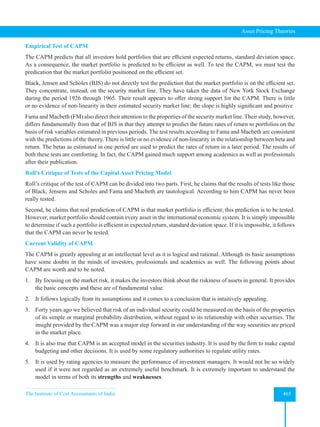
![Strategic Financial Management
466 The Institute of Cost Accountants of India
Benefits and Limitations of CAPM
Benefits - CAPM model of portfolio management can be effectively used to:
(a) Investors can estimate the required rate of return on a particular investment in company’s securities.
(b) Investments in risky projects having real assets can be evaluated of its worth in view of expected return.
(c) CAPM analyses the riskiness of increasing the levels of gearing and its impact on equity shareholders returns.
(d) CAPM suggests the diversification of portfolio in minimization of risk.
Limitations - CAPM is criticized for the following reasons:
(a) In real world, assumptions of CAPM will not hold good.
(b) In practice, it is difficult to estimate the risk free return, market rate of return, and risk premium.
(c) CAPM is a single period model while most projects are often available only as large indivisible projects. It is
therefore more difficult to adjust.
Illustration 7
The following information is available in respect of security A:
Equilibrium return 12%
Market return 12%
6% Treasury bond trading at `120
Co-variance of market return and security return 196%
Coefficient of correlation 0.80
You are required to determine the standard deviation of:
(i) Market return
(ii) Security return
Solution
Rf
= (6/120) × 100 = 5% [Rf
= Risk free return]
Applying CAPM:
12% = 5% + β (Rm
- Rf
)
or 7% = β (12% - 5%)
or β = 1
(i) We know β = [Cov(A, m)] ÷ σ2
m
or 1 = 196 ÷ σ2
m
= 196
or σm
= 14%
Standard deviation of market return = 14%
(ii) Correlation coefficient = [Cov(A, m)] ÷ σm
σA
or 0.80 = 196 ÷ (14 × σA
) or 11.20σA
= 196
Thus, σA
= 17.5%
Standard deviation of security return = 17.5%](https://image.slidesharecdn.com/strategyfamous-230209132502-a14bc8e7/85/Strategy_Famous-pdf-478-320.jpg)
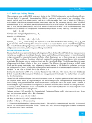
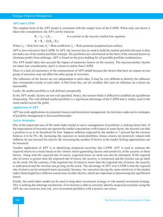
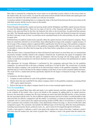
![The Institute of Cost Accountants of India 471
Asset Pricing Theories
To calculate the leveraged beta, we need to know the unlevered beta and the debt-to-equity ratio. Systematic risk
is the risk that affects the overall market. Beta does not take into account the unsystematic risk. Unsystematic risk
specifically affects a stock, so it can be reduced by diversifying the portfolio.
The term “levered beta” refers to the systematic risk of a company stock that is primarily used in the computation
of the expected rate of return using the capital asset pricing model (CAPM). In other words, levered beta takes into
account the impact of the company’s debt level compared to its equity on its systematic risk exposure. Levered beta
is also known as equity beta.
The formula for the levered beta can be derived by multiplying the unlevered beta with a factor of 1 plus the
product of the company’s debt-to-equity ratio and (1 – tax rate). Mathematically, it is represented as,
Levered Beta = Unlevered Beta × [1 + (1 – Tax Rate) × (Debt / Equity)]
9.2.2 Unlevered Beta
It is a risk measurement metric that compares the risk of a company without any debt to the risk of the market. In
simple language, unlevered beta is a company’s beta without considering the debt. It is also referred to as asset
beta because the risk of a firm after removing leverage is because of its assets. Unlevered beta (or ungeared beta)
takes only equity in its capital structure and then compares the risk of a firm to the risk of the market. Unlevered
beta is useful when comparing companies with different capital structures as it focuses on the equity risk and is
also referred to as the “Asset Beta” since its value is determined by the assets (or businesses) owned by the firm,
however, unlevering the beta removes beneficial effects gained by adding debt to the firm’s capital structure.
Generally, the Unlevered beta is lower than the levered beta however, it could be higher in some cases especially
when the net debt is negative (meaning that the company has more cash than debt).
Some industries or companies have a high level of debt on their balance sheet. This leverage makes their earnings
volatile, and investment in this company becomes risky. Levered beta considers the risk of leverage and its impact
on the company’s performance. So, levered beta is not an ideal measure to compare two companies with different
debt proportions. In such a scenario, you will have to remove the effect of debt by “unlevering” the beta. Unlevered
beta will facilitate a better comparison for such companies than levered beta.
Unlevered Beta = Levered Beta ÷ 1 + [ ( 1 –Tax) × ( Debt/ Equity)]
Illustration 8
Assume for the subject company:
Unlevered beta: 0.90
Tax rate: 0.30
Capital structure: 60% debt, 40% equity
Solution:
BL
= 0.90(1 + (1 – 0.30)0.60/0.40)
= 0.90(1 + 0.70(1.5))
= 0.90(2.05)
= 1.85
It is better to use an unlevered beta over a levered beta when a company or investor wishes to measure a publicly-
traded security’s performance in relation to market movements without the effects of that company’s debt factor.
A publicly traded security’s levered beta measures the sensitivity of that security’s tendency to perform in relation
to the overall market. Levered beta includes a company’s debt in the calculation of its sensitivity. Security with
positive levered beta signals that the security has a positive correlation with market performance and security with
negative levered beta signals that the security has a negative correlation with market performance.
A levered beta greater than positive 1 or less than negative 1 means that it has greater volatility than the market. A
levered beta between negative 1 and positive 1 has less volatility than the market.](https://image.slidesharecdn.com/strategyfamous-230209132502-a14bc8e7/85/Strategy_Famous-pdf-483-320.jpg)
![Strategic Financial Management
472 The Institute of Cost Accountants of India
Additional Illustrations
1. If the risk free rate of interest (Rf
) is 10%, and expected return on market portfolio (Rm
) is 15%, ascertain
expected return of the portfolio if portfolio betas are — (a) 0.10 and (b) 0.30.
Solution:
1. Rule for determining Expected Return on Portfolio under CAPM
Under Capital Asset Pricing Model (CAPM) Rp
= Rf
+ [β × (Rm
- Rf
)]
Notation Particulars Value
Rp
Expected Return on Portfolio To be computed
Rf
Risk Free Rate of Interest/ Return 10%
β Portfolio Beta 0.10/0.30
Rm
Expected Return on Market Portfolio 15%
2. Computation of Expected Return on Portfolio
Beta Expected Return = Rf
+ β × (Rm
- Rf
)
0.10 = 10% + 0.10(15% -10%) =10.5%
0.30 = 10% + 0.30(15% - 10%) =11.5%
2. Subho has invested in four securities M, N, O and P, the particulars of which are as follows —
Security M N O P
Amount Invested (`) 1,25,000 1,50,000 80,000 1,45,000
Beta (β) 0.60 1.50 0.90 1.30
If RBI Bonds carries an interest rate of 8% and NIFTY yields 14%, what is the expected return on portfolio?
If investment in Security O is replaced by investment in RBI Bonds, what is the corresponding change in
Portfolio Beta and expected return?
Solution:
(i) Computation of Expected Return on Portfolio (Under CAPM)
(a) Computation of Weighted Beta (Beta of the Portfolio)
Security Amount
Invested (`)
Proportion of Investment to
Total Investment
Beta of Investment Weighted Beta
(1) (2) (3) = (2) ÷ 5,00,000 (4) (5) = (3) × (4)
M 1,25,000 0.25 0.60 0.150
N 1,50,000 0.30 1.50 0.450
O 80,000 0.16 0.90 0.144
P 1,45,000 0.29 1.30 0.377
Total 5,00,000 1.00 1.121](https://image.slidesharecdn.com/strategyfamous-230209132502-a14bc8e7/85/Strategy_Famous-pdf-484-320.jpg)
![The Institute of Cost Accountants of India 473
Asset Pricing Theories
(b) Computation of Expected Return on Portfolio
Expected Return [E(Rp
)] = Rf
+ [βp
× (Rm
– Rf
)]
= 8% + [1.121 × (14% - 8%)]
= 8% + [1.121 × 6%]
= 8% + 6.726%
= 14.726%
(ii) Computation of Expected Return [Investment in O, replaced by RBI Bonds] (CAPM)
(a) Computation of Weighted Beta (Beta of the Portfolio)
Security Amount
Invested (`)
Proportion of Investment to
Total Investment
Beta of Investment Weighted Beta
(1) (2) (3) = (2) ÷ 5,00,000 (4) (5) = (3) × (4)
M 1,25,000 0.25 0.60 0.150
N 1,50,000 0.30 1.50 0.450
RBI Bonds 80,000 0.16 0.00 0.000
P 1,45,000 0.29 1.30 0.377
Total 5,00,000 1.00 0.977
(b) Computation of Expected Return on Portfolio
Expected Return [E(RP)]
= Rf
+ [βp
× (Rm
– Rf
)]
= 8% + [0.977 × (14% - 8%)]
= 8% + [0.977 × 6%]
= 8% + 5.862%
= 13.862%
3. The beta coefficient of M Ltd. Is 1.40. The company has been maintaining 8% rate of growth in dividends
and earnings. The last dividend paid was `4.00 per share. Return on government securities is 12% and return
on market portfolio is 18%. The current market price of the share of M Ltd. Is `32.00. What will be the
equilibrium price per share of M Ltd.?
Solution
Required rate of return as per CAPM = Rf
+ (Rm
- Rf
) × βi
= 12 + (18-12) × 1.40 = 20.40%.
Equilibrium price D1
= 4 × (1+0.08) = 4 × 1.08 = ` 4.32 and G = 0.08 [E.P. = Equilibrium price].
Expected return = [D1
/E.P.] + g or 20.40 = 4.32/E.P. + 0.08
or (0.2040 - 0.08) E.P. = 4.32
or 0.124 E.P. = 4.32
or E.P. = 4.32 / 0.124 or `34.84. or equilibrium price = `34.84](https://image.slidesharecdn.com/strategyfamous-230209132502-a14bc8e7/85/Strategy_Famous-pdf-485-320.jpg)
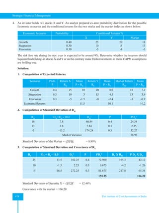
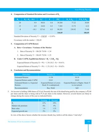
![Strategic Financial Management
476 The Institute of Cost Accountants of India
Solution
The return as per existing data:
Rx
= Rf
+ β(Rm
- Rf
) = 0.12 + .06 × 1.4 = 0.204 or 20.4%.
Substituting this for ke
in the dividend discount model
P =
D0
(1+g)
ke
- g
or P = (2×1.05) / (0.204 – 0.05) = `13.63.
Since the share is selling at ` 25, it is overpriced. He should sell his shares now.
As per the revised data, we should have
Rx
= 0.10 + 1.25 × 0.04 = 15%
Substituting this for ke
in the dividend discount model
P =
D0
(1+g)
ke
- g
we get, P = (2 × 1.09) / (0.15 – 0.09) = ` 36.33.
Since the share is selling at ` 25.00 it is underpriced, he should hold the shares as per revised data.
6. Sanjiv is contemplating buying/selling the shares of Companies M, N and O. He already holds some shares in
each of these Companies. He has the following data in his hand to aid him in his decision —
• Return on NIFTY 16%
• ` 500 Treasury Bonds, whose returns are considered risk free, earns its owners a return of `35
• Company M has a Beta Factor of 0.95 and investment therein yields a return of 13.5%
• Company N, which is traded at `1,200 per shares, earns its investors a sum of `246. It has a beta factor of
1.5.
• Company O, price of which is `450 has a beta factor of 0.6. Historical data shows that annual share price
increase of the Company is around 8%. Last dividend declared was `12 per share. Dividend payout is
expected to double in the next year.
Sanjiv seeks your guidance on the course of action.
Solution:
1. Market Return (RM
) and Risk Free Return (RF
)
(a) Market Return = Return on NIFTY = 16%
(b) Risk Free Return = Return on Treasury Bonds = Return in `/Face Value = `35/`500 =7%
2. Evaluation of Company M
Particulars Value
Estimated Return (Given) (RM
) [A] 13.5%
Expected Return under CAPM [E(RM
)]
E(RM
) = RF
+ βM
X (RM
– RF
) = 7% + 0.95 X (16% - 7%) [B]
15.55%
Estimated Return [A] vs. Expected Return under CAPM [B] [B] is Higher
Inference Stock gives lesser than what is should
give
Conclusion [Expected Return is higher than Estimated
Return] Share is
Overpriced
Recommendation SELL](https://image.slidesharecdn.com/strategyfamous-230209132502-a14bc8e7/85/Strategy_Famous-pdf-488-320.jpg)
![The Institute of Cost Accountants of India 477
Asset Pricing Theories
3. Evaluation of Company N
Particulars Value
Estimated Return (Given) `246
Market Price (Given) `1200
Estimated Return (in %) (RN
) [Estimated Return `246/Market Price `1200][A] 20.50%
Expected Return under CAPM [E(RN
)]
E(RN
) = RF
+ βN
× (RM
– RF
) = 7% + 1.50 × (16% - 7%) [B]
20.50%
Estimated Return [A] vs. Expected Return under CAPM [B] Equal
Inference Stock is giving
exactly what it
should give
Conclusion [Expected Return is EQUAL To Estimated Return] Share is Correctly priced
Recommendation HOLD
4. Evaluation of Company O
Particulars Value
Capital Appreciation Expected (Market Price of `450 × 8%) `36
Estimated Dividend Payout (Previous Year’s Dividend of `12 × 2 Times) `24
Total Estimated Return for the year `60
Estimated Return (in %) (RO
) [Estimated Return `60/Market Price `450][A] 13.33%
Expected Return under CAPM [E(RB
)]
E(RO
) = RF
+ βO
× (RM
– RF
) = 7% + 0.60 × (16% - 7%) [B]
12.40%
Estimated Return [A] vs. Expected Return under CAPM [B] [B] is lower
Inference Stock gives more than
what it should give
Conclusion [Expected Return is LOWER than Estimated Return] Share is Underpriced
Recommendation BUY
7. You have chosen a risky market portfolio P, with an expected return of 15% and a standard deviation of 25%.
The Rf
0.06.
(a) State the equation for CML for portfolio P
(b) Suppose you prefer to reduce your risk by investing 40% in Rf
,and balance 60% in portfolio P. What is
your expected return now?
(c) What is your risk as per (b) above.](https://image.slidesharecdn.com/strategyfamous-230209132502-a14bc8e7/85/Strategy_Famous-pdf-489-320.jpg)
![Strategic Financial Management
478 The Institute of Cost Accountants of India
Solution
(a) We know that CML is a graph plotting returns on y axis versus (σ) standard deviation (x axis). It joins Rf
,
plotted on the y axis and is drawn as a tangent to the maximum variance portfolio (efficient set), joining Rf
and any other risky portfolio (in this case portfolio P).
This equation is given by:
E(Rp
) = 0.06 + [(0.15 - 0.06) ÷ 0.25]σP
or E(Rp
) = 0.06 + 0.36σP
[Slop = (0.15 - 0.06)/0.25; y intercept = 0.06]
(b) E(Rp
) = 0.40 × 0.06 × 0.60 × 0.15 = 0.024 + 0.09 = 11.4%
(c) σP
= 0.06 × 0.25 + 0.40 × 0 = 15%.
8. Assume the asset below is correctly priced according to security market line. Device the SML. What is the
expected return on an asset with a beta of 2?
R1
= 6%; R2
= 12%; β1
= 0.5; β2
= 1.5
Solution
Since the SML is linear, we need only two points:
Ri
= Rf
+ βi
(Rm
– Rf
)
6% = Rf
+0.5(Rm
– Rf
) = 0.5Rf
+0.5Rm
12% = Rf
+1.5(Rm
– Rf
) = -0.5Rf
+1.5Rm
Adding the equations:
18% = 2.0 Rm
or Rm
= 9%
Thus, Rf
= [6-0.5(9)]/0.5 = 3% [Putting the value in equation (i)]
Hence, the SML is: βi
= 3% + βi
(9 – 3) or 3% + 6βi
For beta = 2;
Ri
= 3 + 2(6) = 15%
9. Tea Ltd., has been enjoying a substantial net cash inflow, and until the surplus funds are needed to meet tax and
dividend payments, and to finance further capital expenditure in several months time, they have been invested
in a small portfolio of short-term equity investments.
Details of the portfolio, which consists of shares in four UK listed companies, are as follows.
Company
Number of
shares held
Beta equity
coefficient
Market price
per share (`)
Latest Dividend
yield (%)
Expected return on
equity in the next year %
A Ltd.
B Ltd.
C Ltd.
D Ltd.
60,000
80,000
1,00,000
1,25,000
1.20
2.30
0.85
1.28
4.29
2.92
2.17
3.14
6.10
3.40
5.70
3.30
19.50
24.00
17.50
23.00
The current market return is 19% a year and the Risk free rate is 11% a year.
Required:
1. On the basis of the data given, calculate the risk of Tea Ltd’s short term investment portfolio relative to
that of the market.
2. Recommend, with reasons, whether Tea Ltd., should change the composition of its portfolio.](https://image.slidesharecdn.com/strategyfamous-230209132502-a14bc8e7/85/Strategy_Famous-pdf-490-320.jpg)
![The Institute of Cost Accountants of India 479
Asset Pricing Theories
Solution:
(1) Computation of Weighed Beta
Security
No. of
shares held
MPS
(`)
Market value
of investments
Proportion Beta
Portfolio
Beta
[1] [2] [3] [4] [5] [6] [7] = [5] ×
[6]
A
B
C
D
60,000
80,000
1,00,000
1,25,000
4.29
2.92
2.17
3.14
2,57,400
2,33,600
2,17,000
3,92,500
2,57,400 ÷ 11,00,500 = 0.2339
2,33,600 ÷ 11,00,500 = 0.2123
2,17,000 ÷ 11,00,500 = 0.1972
3,92,500 ÷ 11,00,500 = 0.3567
1.20
2.30
0.85
1.28
0.28068
0.48829
0.16762
0.45658
11,00,500 1 5.63 1.393166
(2) Comparison with Return under CAPM and Recommended changes in Composition
Security Valuation under CAPM = RF
+ [β×(RM
– RF
)]
Expected Ke
in
the next year %
Evaluation Strategy
A 11% + 1.20 (19% - 11%) = 20.60 19.50 Overpriced Sell
B 11% + 2.30 (19% - 11%) = 29.40 24.00 Overpriced Sell
C 11% + 0.85 (19% - 11%) = 17.80 17.50 Overpriced Sell
D 11% + 1.28 (19% - 11%) = 21.24 23.00 Under priced Buy
10. Share of Sharee Limited has a beta factor of 1.8. The NIFTY has yielded a return of 17.5%. 6.75% `100
Treasury Bills are traded at `108. Ascertain —
(a) Expected Return on Shares of Sharee Ltd under CAPM.
(b) Alpha Factor of Shares of Sharee Ltd if the past 5 Years actual returns on shares of Sharee Ltd are —
23.4%; 27.2%; 26.6%; 24.3% and 28.5%.
Solution:
1. Expected Return on Shares of Sharee Ltd [E(RS
)] (Under CAPM)
(a) Computation of Risk Free Return (RP
)
Particulars Value
Face Value of Treasury Bills
Return on Face Value (in %)
Return on Treasury Bills (in Value) [`100 × 6.75%]
Trading Price of Treasury Bills
Risk Free Return (RF
) as per Market Expectations [Actual Return `6.75/Market Price `108]
`100
6.75%
`6.75
`108
6.25%
(b) Expected Return [E(RS
)]
E(RS
) RF
+ [βV
× (RM
– RF
)]
Risk Free Return RF
6.25% [As per Working Note 1(a)]
Return on Market Portfolio RM
17.5% [Return on NIFTY]
Beta Factor βV
1.80 [Given]](https://image.slidesharecdn.com/strategyfamous-230209132502-a14bc8e7/85/Strategy_Famous-pdf-491-320.jpg)
![Strategic Financial Management
480 The Institute of Cost Accountants of India
E(RS
) = RF
+ [βV
× (RM
– RF
)]
= 6.25% + [1.80 × (17.5% – 6.25%)]
= 6.25% + [1.80 × 11.25%]
= 6.25% + 20.25
= 26.5%
2. Value of Alpha (αv
) for Return on Shares of Sharee Ltd [E(RS
)]
Year Actual Return Abnormal Return [ARS
]
(1) (2) (3) = (2) – E(RS
)
1
2
3
4
5
23.4
27.2
26.6
24.3
28.5
23.4% – 26.50% = (3.10%)
27.2% – 26.50% = 0.70%
26.6% – 26.50% = 0.10%
24.3% – 26.50% = (2.20%)
28.5% – 26.50% = 2.00%
Total (2.50%)
∝V =∑ARS
÷ n = (2.50%) ÷ 5 Years = (0.50%)
Inference:Alpha is negative. Therefore, expected return will be less than return under CAPM to the extent
of 0.50%.
11. Returns on two portfolios, B and L, for the past 4 years are —
Year 1 2 3 4
Portfolio B
Portfolio L
13.00%
14.35%
13.50%
11.75%
12.50%
13.60%
14.00%
12.90%
Beta factor of the two portfolios are 1.3 and 1.2 respectively. If the market portfolio fetches 12% return and
RBI Bonds, which are considered risk free, yield 5% return, which of the above two portfolios will an investor
prefer?
Solution:
1. Computation of Expected Rate of Return under CAPM
E(RX
) RF
+ [βX
× (RM
– RF
)] [Expected Return on Portfolio X]
Risk Free Return RF
5% [Treasury Bills]
Return on Market Portfolio RM
12% [Given]
Expected Return on Portfolio B Portfolio L
Beta Factor 1.30 1.20
Expected Return E(RB
) = RF
+ [βB
× (RM
– RF
)]
= 5% + [1.30 × (12% - 5%)]
= 5% + [1.30 × 7%]
= 5% + 9.1% = 14.10%
E(RL
) = RF
+ [βL
× (RM
– RF
)]
= 5% + [1.20 × (12% - 5%)]
= 5% + [1.20 × 7%]
= 5% + 8.4% = 13.40%](https://image.slidesharecdn.com/strategyfamous-230209132502-a14bc8e7/85/Strategy_Famous-pdf-492-320.jpg)
![The Institute of Cost Accountants of India 481
Asset Pricing Theories
2. Computation of Alpha Factors
Year
Portfolio B Portfolio L
Actual Return Abnormal Return [ARB
] Actual Return Abnormal Return [ARL
]
(1) (2) (3) = (2)-E(RB
) (4) (5) = (4)-E(RL
)
1
2
3
4
13.00%
13.50%
12.50%
14.00%
13.00% - 14.10% = (1.10%)
13.50% - 14.10% = (0.60%)
12.50% -14.10% = (1.60%)
14.00% -14.10% = (0.10%)
14.35%
11.75%
13.60%
12.90%
14.35% - 13.40% = 0.95%
11.75% - 13.40% = (1.65%)
13.60% - 13.40% = 0.20%
12.90% - 13.40% = (0.50%)
(3.40%) (1.00%)
Alpha Factor:
Portfolio B ∝B
= ∑ARB
÷ n = ((3.40%) ÷ 4 Years = (0.85%)
Portfolio L ∝L
= ∑ARL
÷ n = ((1.00%) ÷ 4 Years = (0.25%)
3. Expected Return adjusted for Alpha
Alpha Adjusted Return = Return under CAPM + ∝
Portfolio B = E(RB
) + aB
= 14.10% - 0.85% = 13.25%
Portfolio L = E(RL
) + aL
= 13.40% - 0.25% = 13.15%
Conclusion: The Alpha for Security B is higher than L, indicating its better performance relative to L.
Hence, an investor should prefer Portfolio B.
12. Estimate the stock return by using CAPM and the APT model by which the particulars are given below:
(a) The expected return of the market is 14 per cent and the equity beta is 1.2. The risk free rate of interest is
6 per cent.
(b)
Factor Market Price of Risk (%) Sensitivity Index
Inflation 5 1.2
Industrial Production 1 0.9
Risk Premium 3 1.1
Interest Rate 4 -0.8
What explanations can you offer for the difference in the two estimates?
Solution:
Return as per CAPM
(a) Ri
= Rf
+ (Rm
- Rf
) × βi
= 0.06 + (0.14 - 0.06) × 1.2
= 0.06 + 0.096
= 0.156
= 15.60%.
Return under APT Model](https://image.slidesharecdn.com/strategyfamous-230209132502-a14bc8e7/85/Strategy_Famous-pdf-493-320.jpg)
![Strategic Financial Management
482 The Institute of Cost Accountants of India
(b) Ri
= λ0
+ [λ1
βi1
+ λ2
βi2
+ λ3
βi3
+ λ4
βi4
]
= 0.06 + [0.05 × 1.2 + 0.01 × 0.9 + 0.03 × 1.1 + (0.04 × -0.8)]
= 0.06 + [0.06 + 0.009 + 0.033 - 0.032]
= 0.06 + [0.07]
= 0.13 or 13%
The rates are different under two models due to the usage of different variables. The rate under APT is
much lower because of negative impact of interest rate factor.
13. Mr. Parekh is totally confused whether he should purchase stock of HUL or not. His financial analyst has
provided the following information:
Rƒ
= 5%
Factor λi
βi
Interest Rate Risk 0.90 0.90
Purchasing Power Risk 0.8 1.70
Inflation Risk 1.4 1.50
Market Risk 0.7 -1.60
The probability of getting a return on HUL stock is given below:
Return % Probability (%)
18 40
20 30
12 20
8 10
Advise Mr. Parekh.
Solution
The expected return on stock of HUL based on APT is
Ri
= λ0
+ [λ1
βi1
+ λ2
βi2
+ λ3
βi3
+ λ4
βi4
]
= 6 + [0.90 x 0.90 + 0.80 x 1.70 + 1.4 x 1.50 + (0.70 x -1.60)]
= 6 + [0.81 + 1.36 + 2.1 - 1.12]
= 6 + 3.15
= 9.15%
The probable return = 18 x 0.40 + 20 x 0.30 + 12 x 0.20 + 8 x 0.10
= 7.20 + 6.00 + 2.40 + 0.80 = 16.40%
As probable return is much higher, Mr. Parekh should buy HUL stock.](https://image.slidesharecdn.com/strategyfamous-230209132502-a14bc8e7/85/Strategy_Famous-pdf-494-320.jpg)
![The Institute of Cost Accountants of India 483
Asset Pricing Theories
14. The estimated factor sensitivities of ITC to the five macroeconomic factors are given below along with market
risk premium to each of these factors.
Factor Sensitivity Risk Premium (%)
Default risk 0.25 2.60
Inflation risk 0.32 -0.70
Business cycle risk 1.60 1.80
Time horizon risk 0.40 -0.75
Market-timing risk 0.90 3.17
Use the APT model to calculate the required rate of return for ITC assuming that treasury bill rate is 4.5%.
Solution
Return under five factor APT model will be:
E(Ri
) = Rƒ
+ (Default risk sensitivity × Risk premium) + (Inflation risk sensitivity × Risk premium) +
(Business cycle risk sensitivity × Risk premium) + (Time horizon sensitivity × Risk premium) + (Market
timing sensitivity × Risk premium)
E(Rƒ
) = 4.5 + (0.25 × 2.60) + (0.32) × (-0.70) + (1.60 × 1.80) + (0.40 × -0.75) + (0.90 × 3.17)
= 4.5 + [0.65 - 0.224 + 2.88 - 0.30 + 2.853]
= 4.5 + 5.859
= 10.36%
Solved Case Studies
1. A portfolio management services manages a stock fund consisting of five stocks with the following market
values, betas and expected returns:
Stock Market value (`) Beta Expected Return
A 2,00,000 1.10 15%
B 1,00,000 0.75 14%
C 1,50,000 0.90 15%
D 2,50,000 1.20 16%
E 3,00,000 1.40 17%
If risk free rate of return is 9% and expected return on market is 15%:
(a) What is the portfolio expected return as per CAPM?
(b) Which stocks are undervalued or overvalued?
Solution
In order to calculate the fund’s expected return with CAPM, we need the fund’s beta. This can be determined
with the following equation.
βρ
= Wi
Bi](https://image.slidesharecdn.com/strategyfamous-230209132502-a14bc8e7/85/Strategy_Famous-pdf-495-320.jpg)
![Strategic Financial Management
484 The Institute of Cost Accountants of India
Wi
is the weight for the ‘i’th security and Bi
, is the beta co-efficient of the ‘i’th security.
WA
= 2,00,000/10,00,000 = 0.20
WB
= 1,00,000/10,00,000 = 0.10
Wc= 1,50,000/10,00,000 = 0.15
WD
= 2,50,000/10,00,000 = 0.25
WE
=3,00,000/10,00,000 = 0.30
1.00
βρ
= (0.20) (1.1) + (0.10) (0.75) + (0.15) (0.90) + (0.25) (1.20) + (0.30) (1.40)
= 0.22 +0.075 +0.135 +0.3 +0.42 = 1.15
E(Rp
) = Rf
+ [(ERm
- Rf
)] × ßp
= 9 + (15 − 9) × 1.15 = 15.90%.
(b) To find whether the stock is undervalued or overvalued we should first determine the return for each stock
that is consistent with equilibrium using the CAPM.
E(Ri
) = Rf
+ (Rm
− Rf
) × ßi
E(RA
) = 9 + (15-9) × 1.10 = 15.60% (overvalued)
E(RB
) = 9 +(15-9) × 0.75 = 13.50% (undervalued)
E(RC
) = 9 +(15-9) × 0.90 = 14.40% (undervalued)
E(RD
) = 9 +(15-9) × 1.20 = 16.20% (overvalued)
E(RE
) = 9 +(15-9) × 1.40 = 17.40% (overvalued)
Securities A, D and E are overvalued because the expected return is less than the equilibrium return,
whereas securities B and C are undervalued because their equilibrium return is less than their expected
value.
2. XYZ Ltd pays no taxes and is entirely financed by equity shares. The equity share has a beta of 0.6, a price-
earnings ratio of 5 and is priced to offer an expected return of 20%. XYZ Ltd. now decides to buy back half of
the equity shares by borrowing an equal amount. If the debt yields a risk free return of 10%, calculate:
(a) The beta of the equity shares after buy back.
(b) The required return and risk premium on the equity shares before the buy back.
(c) The required return and risk premium on the equity shares after buy back.
(d) The required return on debt.
(e) The percentage increase in expected earnings per share.
(f) The new price-earnings multiple.
Assume that operating profit of the firm is expected to remain constant in perpetuity.
Solution:
Before buy back – Beta = 0.6; P/E = 5; ER
(i) = 20%; Rf
= 10%
(a) Beta of equity share after buy back
βA
= [βE
×
E
D+E ]×[βD
×
D
D+E ]
Or, 0.6 = 0.5 × βE
+ 0.5 × 0.
Or, βE
= 1.20.](https://image.slidesharecdn.com/strategyfamous-230209132502-a14bc8e7/85/Strategy_Famous-pdf-496-320.jpg)
![The Institute of Cost Accountants of India 485
Asset Pricing Theories
(b) Calculation of required return and the risk premium on the equity shares before the buyback.
Since the entire financing is in equity, its expected return would be 20%
E(R(i)
) = Rf
+ ß(Rm
- Rf
). Let X be the risk premium
0.20 = 0.10+ 0.60 × X
X = 0.10/0.6 = 16.67%.
(c) Calculation of required return and the risk premium on the equity shares after buyback
RA
= [RA
×
E
D+E ]×[RD
×
D
D+E ]
Or 0.20 (0.5 × RE
) + (0.5 × 0.10) or RE
= 30%.
E(Ri
) = Rf
+ β(Rm
- Rf
).
Let X be the risk premium
0.30 = 0.10 + 1.2X or X= 16.67%.
(d) The required return on debt is 10%.
(e) Calculation of percentage increase in EPS
Particulars Before Buyback After Buyback
Equity 100 50
Debt @ 10% 0 50
Total 100 100
EBIT@20% 20 20
Interest 0 5
EBT 20 15
Tax 0 0
EAT 20 15
No. of shares 100 50
EPS 0.2 0.3
P/E ratio 5 3.3
Percentage increase in EPS = 50%
(f) The new P/E multiple is 3.33.
3. Mr. Shiva has estimated probable returns under different macroeconomic conditions for the following three
stocks.
Name of the stocks
Current market
price (`)
Rates of return under different macroeconomic scenarios (%)
Recession Moderate growth Boom
X 10 -12 15 35
Y 30 20 12 -5
Z 80 18 20 15
Mr. Shiva is exploring if it is possible to make any arbitrage profits from the above information.
Using the above information construct an arbitrage portfolio and show the payoffs under different economic
scenarios.](https://image.slidesharecdn.com/strategyfamous-230209132502-a14bc8e7/85/Strategy_Famous-pdf-497-320.jpg)