Statistics Project Report

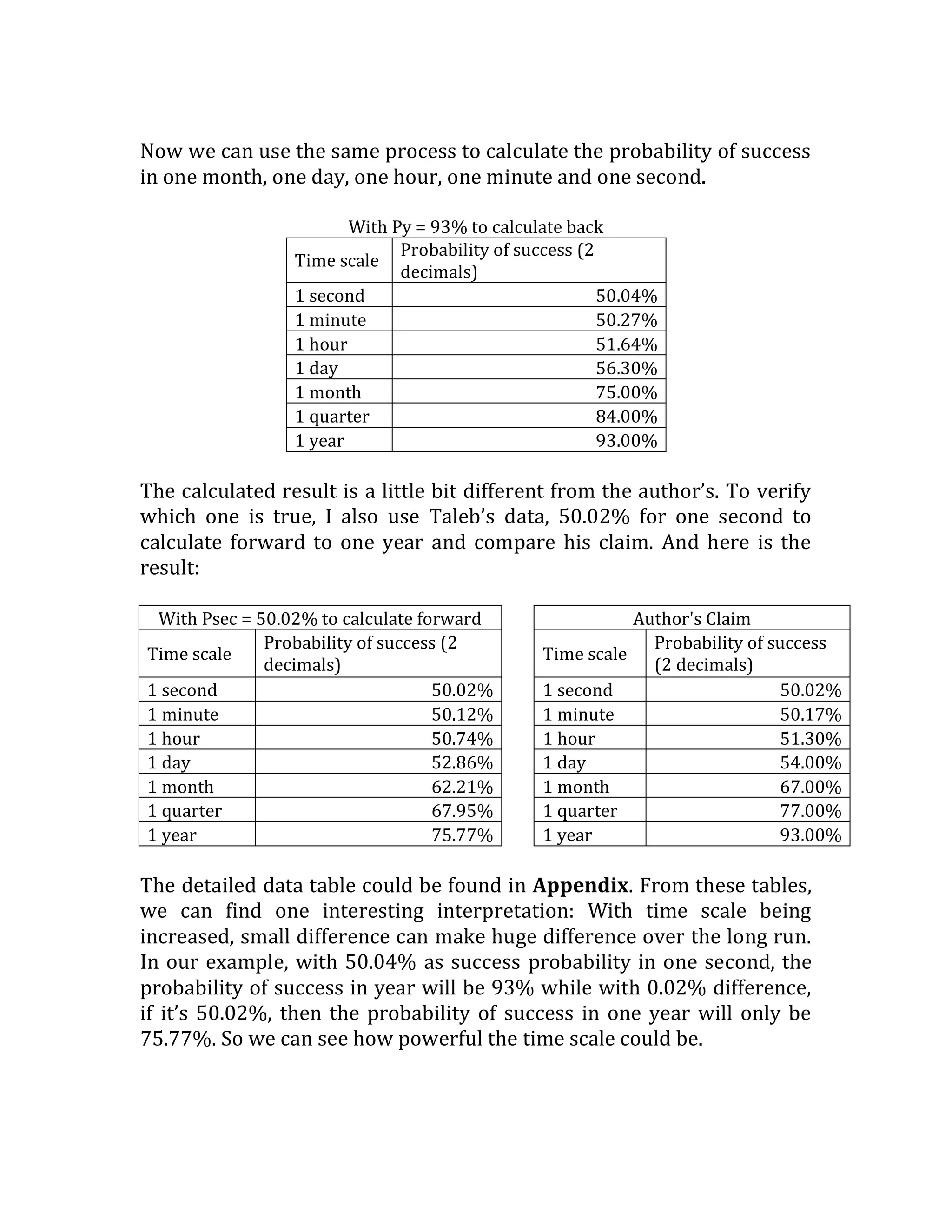
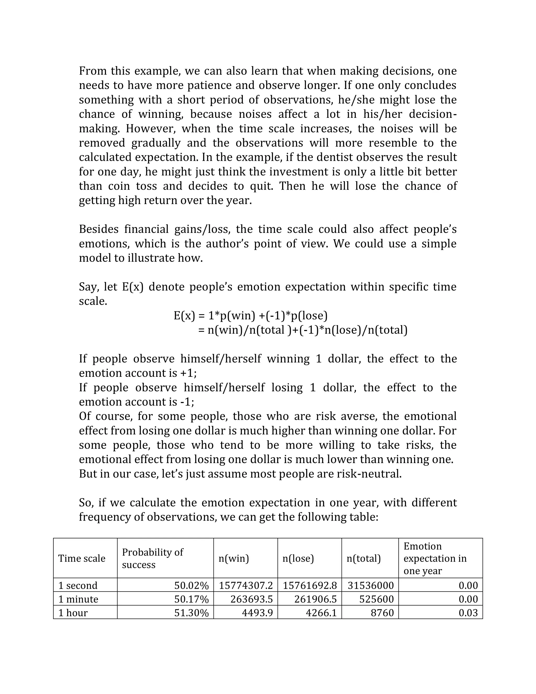
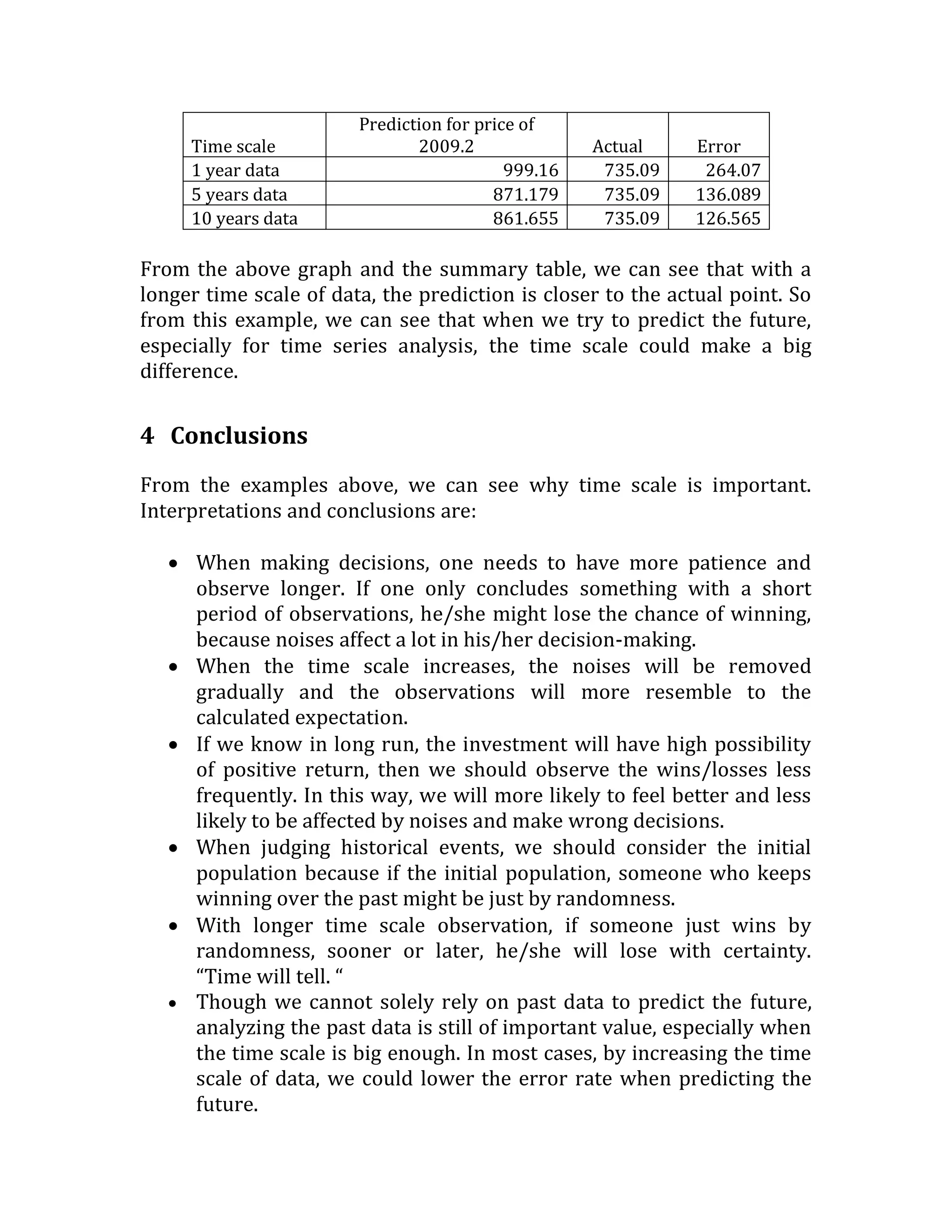
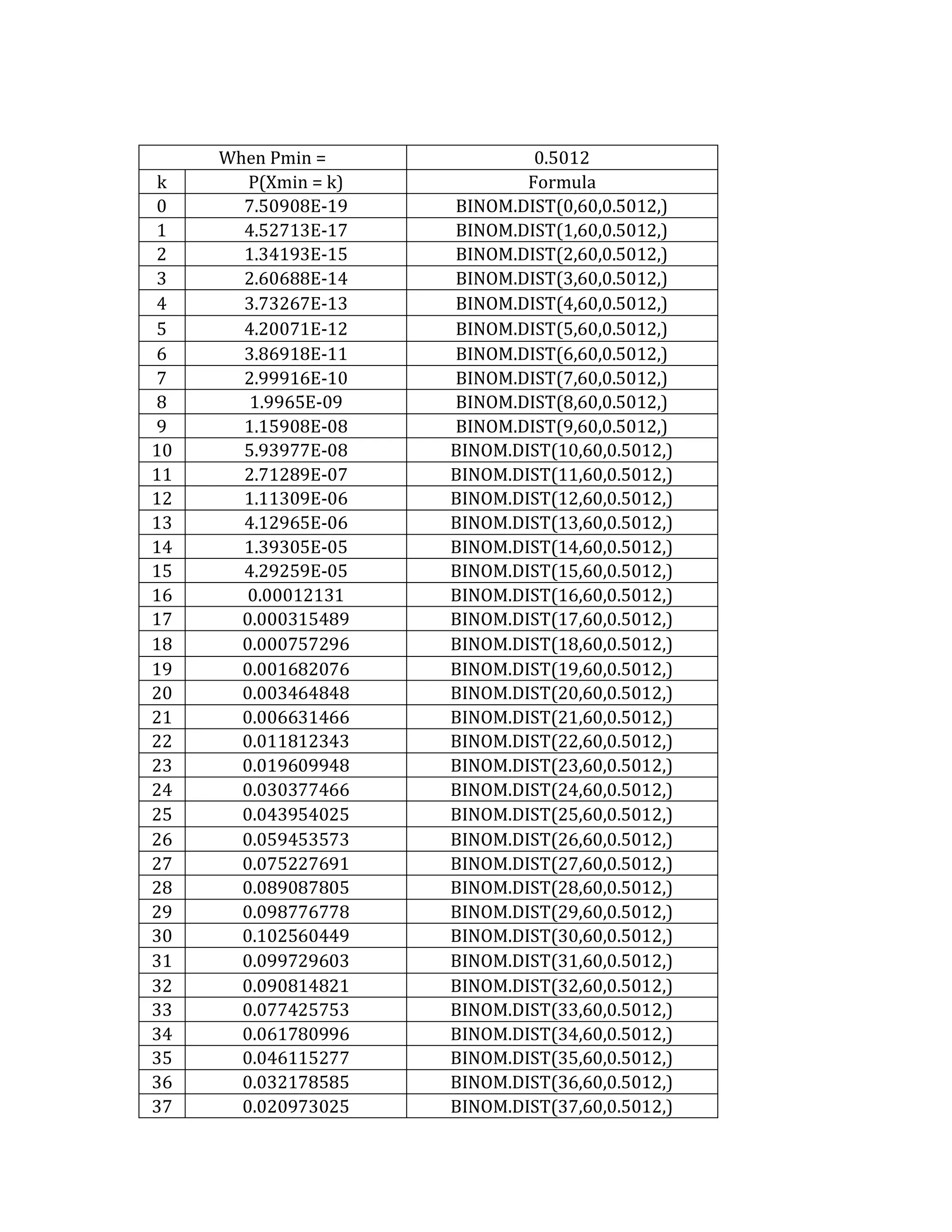
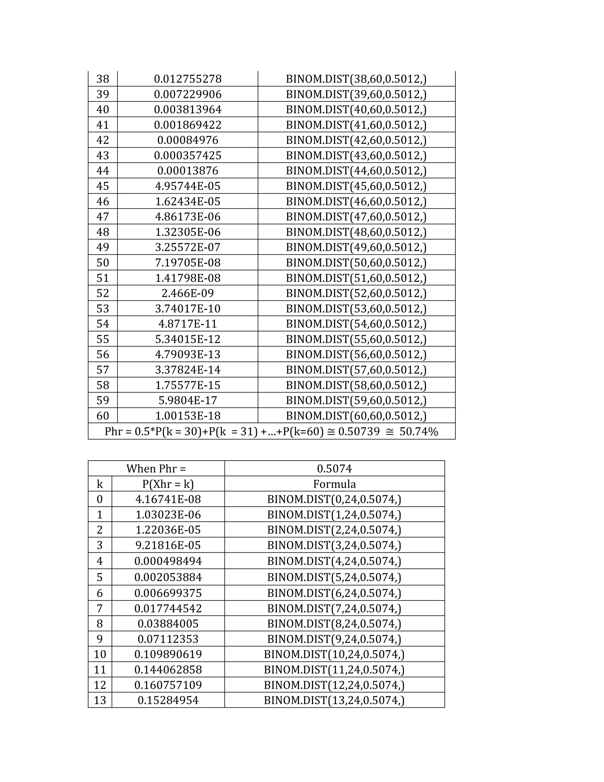
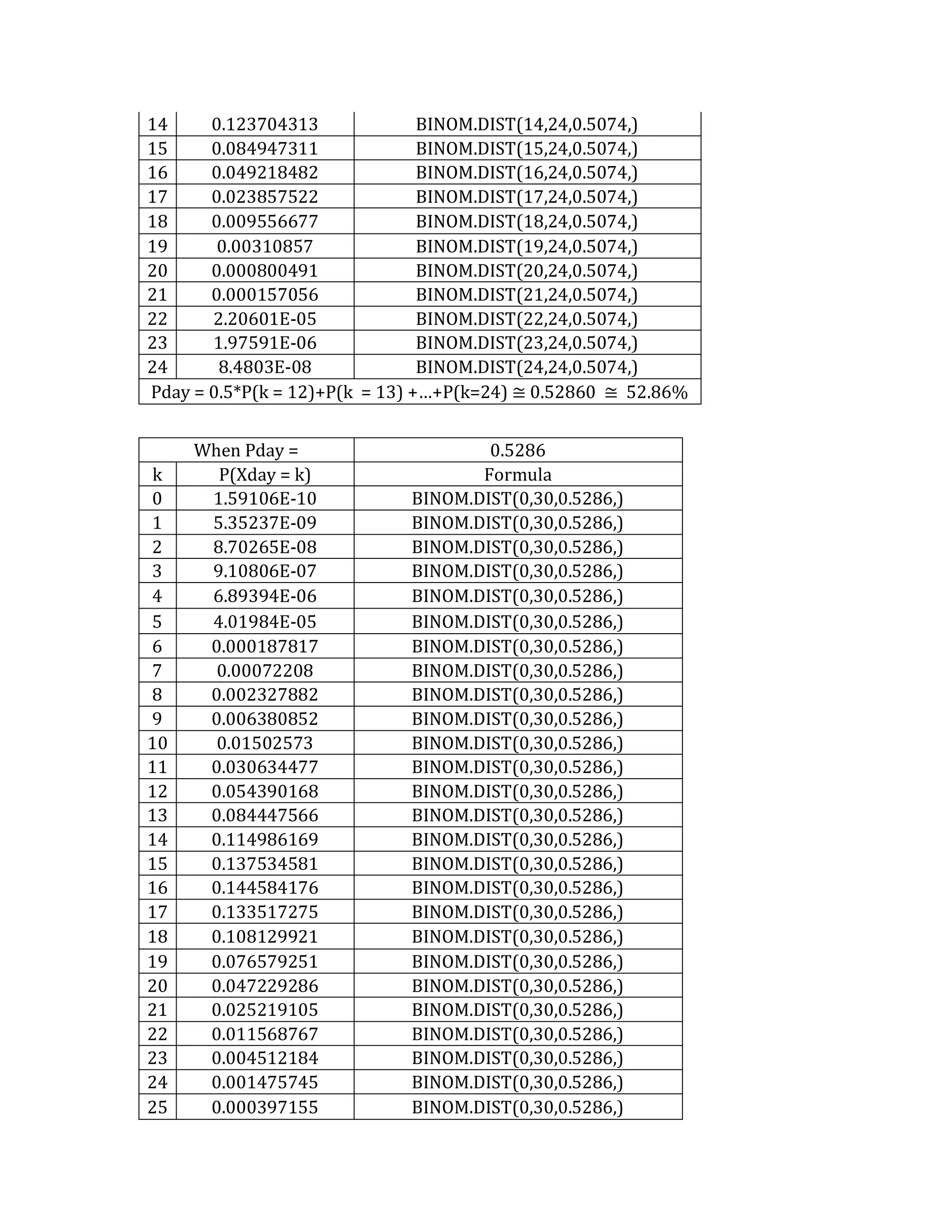
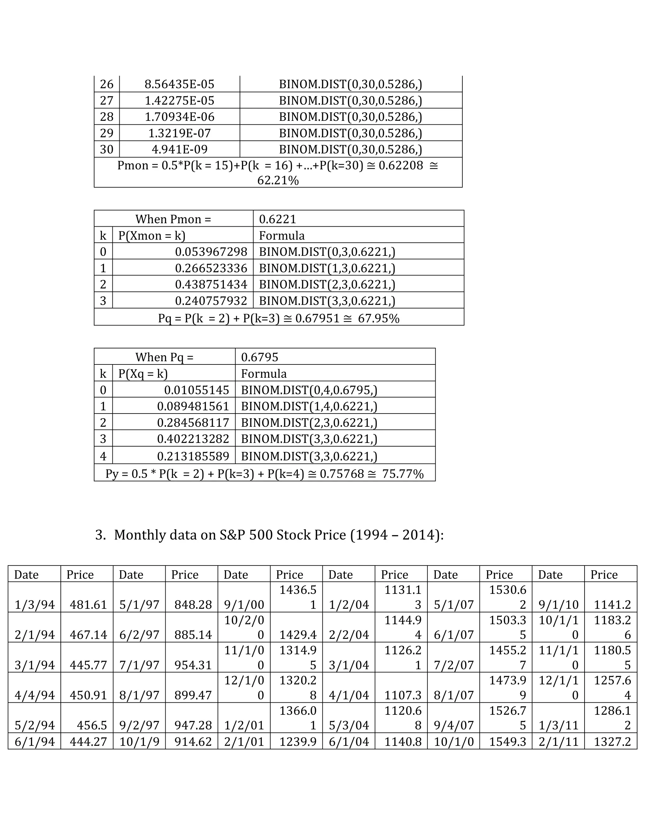
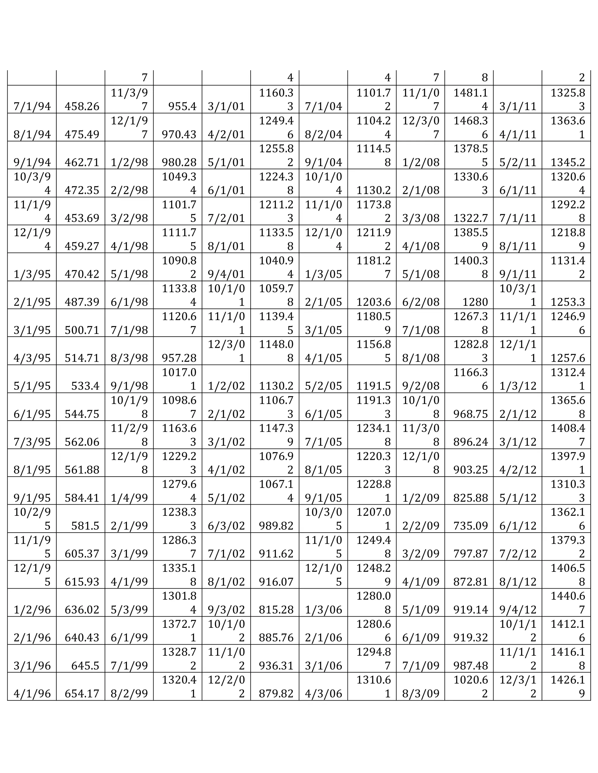
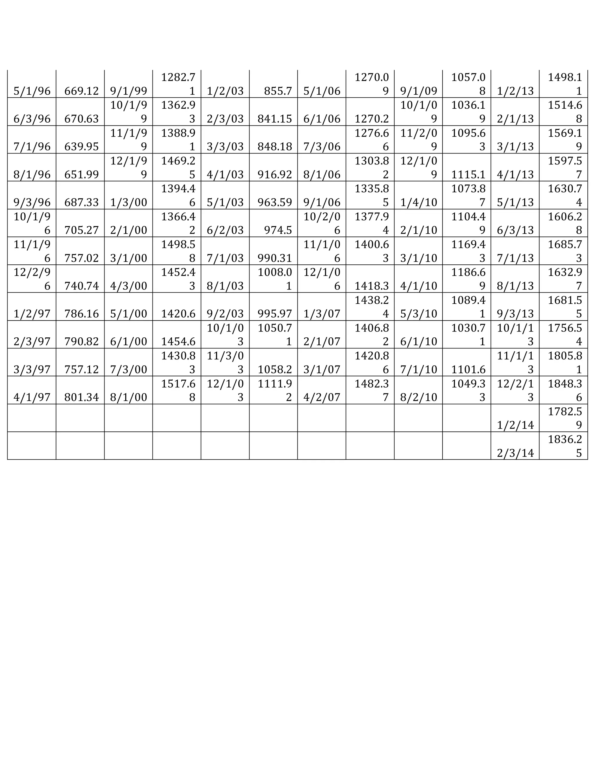
1. ENGS 93: Statistical Methods in Engineering
Final Project
Topic: Why Time Scale Matters?
Book name: <Fooled by Randomness>
Huilian (Irene) Zhang
2014.2.24

2. Contents
1. Book Summary ..................................................................................................................................... 3
2. Project Topic: Why Time Scale Matters?.................................................................................. 6
2.1. Project Goal .................................................................................................................................... 6
2.2. Project Overview & Methodology ....................................................................................... 6
3. Statistical Analysis .............................................................................................................................. 7
3.1 Examination of Examples in the Book .............................................................................. 7
3.1.1 Example 1 .............................................................................................................................. 7
3.1.2 Example 2 ........................................................................................................................... 11
3.2 Real World Data Analysis (Time Series Analysis) .................................................... 14
4 Conclusions ......................................................................................................................................... 17
Appendix......................................................................................................................................................... 18
Bibliography ................................................................................................................................................. 31

3. 1. Book Summary
Written by Nassim Nicholas Taleb, who spent around 20 years as a trader before becoming an academic researcher in probability theory, <Fooled By Randomness> ‘s main idea is that people tend to underestimate the impact of randomness in their lives.
There’re 14 chapters in this book and they are divided into three parts.
Part I (Chapter 1 – Chapter 7) describes situations where people do not understand the rare events. When people have success, they tend to attribute this with some reasons other than pure luck. People tend to underestimate randomness in one’s life because it seems logic counterintuitive to people. Also, it’s in this part that Taleb introduces the concept of black swan and skewness: “It doesn’t matter how frequently something succeeds if failure is too costly to bear.”
In Chapter 1, the author uses a story of two traders, with opposite characters, different attitude towards risk, and different endings, to illustrate how randomness affects them. One of the most inspiring and insightful arguments in this chapter is that we cannot judge the success of people only by their previous performance and personal wealth, because at any point in time, a large section of businessmen with outstanding track records could be just simply because of luck.
In Chapter 2, to illustrate the concept of alternative histories, an example of Russian Roulette is given: One can earn $10 million with 5/6 chance but meanwhile, 1/6 change of being killed. In Taleb’s opinion, $10 million earned through Russian roulette does not have the same value as $10 million earned through the diligent and artful practice of dentistry. In other words, though quantitatively the same, they are qualitatively difference, because one’s dependence on randomness is much greater than the other.
In Chapter 3, Taleb introduces how we could use Monte Carlo simulation to understand a sequence of random historical events. The author argues that we should think about history in mathematical perspective. Here, he introduces the concept of ergodicity, which means, very long sample paths would end up resembling each other. One

4. example to explain this theory is: those who were unlucky in spite of their skills would eventually rise while the lucky fool who might have benefited from some luck in life, over the long run, would slowly converge to the state of a less-lucky guy.
In Chapter 4, this is an extension on how Monte Carlo generator could produce artificial thinking and compare it with rigorous nonrandom constructs.
In Chapter 5, the author uses some examples to show how “Darwinism” and evolution are misunderstood in the non-biological world. Some people believe that an animal is at the maximum fitness for the conditions of its time. However, this is not true, not every single of them. An animal could have survived because of overfitness to a sample path. However, if the time scale is extended to infinity, then, by ergodicity, that rare event will happen with certainty – the species will be wiped out!
In Chapter 6, the author contends that because of psychological bias, people often get confused about probability and expectation, especially when the probability distribution is not symmetric.
In Chapter 7, the problem of induction is discussed. People tend to generalize facts from observations. However, without a proper method, empirical observations can lead people astray. So the need for some rigor in the gathering and interpretation of knowledge, which is called epistemology, is very important.
Part II (Chapter 8 – Chapter 11) is a synthesis review of literature on the subject: the biases of randomness.
In Chapter 8, the author gives three examples to illustrate the survivorship biases which arise from the fact that we only focus on winners and get a distorted view of the odds.
In Chapter 9, some well-known counterintuitive properties of performance records and historical time series are discussed: Survivorship bias, data mining, data snooping, over-fitting, regression to the mean, basically situations where the performance is exaggerated by

5. the observer, resulting from a misperception of the importance of randomness.
In Chapter 10, Taleb argues that life is unfair in a nonlinear way. He gave two examples of two extremes in life: how a small advantage in life can translate into a highly disproportionate payoff, and how randomness can help some people to gain huge sums of money.
In Chapter 11, Taleb contends that as human beings, we tend to be probability blind. Our gene, the media noise, all contributes to the cognitive biases. Taleb illustrates some manifestations of such blindness, with a cursory exposition of the research in this area.
Part III (Chapter 12 – Chapter 14) is the conclusion part of the whole book. It presents the human aspect of dealing with uncertainty. And the author gives some suggestions or in his words, tricks, on how to manage uncertainty in life.
In Chapter 12, Taleb argues that people usually cannot view things as independent from each other and they almost always try to establish a causal link between them from observations, although in fact, those observations may only just come from noise. In addition, people are all quite emotional and derive most of energy from emotions, which may lead them to make wrong decisions, or at least, not rational decisions according to the probability and expectations.
In Chapter 13, Taleb argues that science is great, but individual scientists are dangerous because they are humans who are marred by their psychological biases. In some occasions, they may defend themselves rather than be a pure truth seeker.
In Chapter 14, Taleb discusses randomness from a new angle, with a more archaic type of philosophy, the various guidelines that the ancients had concerning the manner in which a man of virtue and dignity deals with randomness.

6. 2. Project Topic: Why Time Scale Matters?
2.1. Project Goal
One of the most interesting and insightful arguments that I found when reading this book is that, when judging a historical event, the time scale is very important.
So for this project, my focus would be using statistical analysis to demonstrate why people should pay attention to the time scale when making decisions.
2.2. Project Overview & Methodology
Firstly, I would focus on using statistical analysis to examine some of the examples that related to the effect of time scale in this book. For this part, I would use probability distribution theories to calculate the probability of the events mentioned as examples in the book, to see whether I could reproduce the same number as the author’s. In this way, I could validate the author’s arguments.
Secondly, I would extend the analysis to the real world example, which is the historical S&P 500 Price data. Taleb argues that in many cases, time series analysis, or Econometics, is useless. (Page 108, “As a skeptic, I reject a sole time series of the past as an indication of future performance; I need a lot more than data.” Page 112, “I am now convinced that, perhaps, most of econometrics could be useless – much of what financial statisticians know would not be worth knowing.”) Admittedly, relying solely on past data to predict the future is risky, but still, in my opinion, analyzing the past data is of important value, especially when the time scale is big enough, in most cases, we could lower the error rate when predicting the future. To demonstrate my point, I would use Minitab to perform time series analysis with the historical S&P 500 Price data.
Last but not least, several interpretations from the above statistical analysis and how we could apply them when making decisions in life would be summarized.

7. 3. Statistical Analysis
3.1 Examination of Examples in the Book
3.1.1 Example 1
On page 65, there is an interesting table called probability of success at different scales. The example story is that there is a happily retired dentist who made an investment, which has a return rate of 15% and 10% error rate per annum. In a spectrum of one year, we could use normal distribution to approximate the probability of success.
Let X denote the return rate of the investment.
The probability of success in 1 year equals to: P (X>0)
So here, 휇=15,휎=10
푧0= 0−1510= −1.5
1
P (X>0) = 1 – P (푧0)
With z table, we can find that P (푧0) = 0.066807. So,
P (X>0) = 1 – 0.066807 = 0.933191 = 93.3191%
In this book, Taleb said that a 93% probability of success in any given year could be translated into a mere 50.02% probability of success over any given second. (Page 65).
Now let’s try to calculate the numbers backward and see whether we could get the 50.02%.
For this calculation, I would use the binomial distribution, because when the scale becomes smaller, we cannot use normal distribution to approximate binomial distribution.
Let Xq denote the number of quarters (4 quarters in 1 year) that the dentist wins over a year. Then

8. P (X>0) = 0.5*P (Xq = 2) + P (Xq = 3) + P (Xq = 4)
The reason there is a 0.5 in the equation is that when the dentist wins 2 quarters and loses two quarters, the probability of winning over these 4 quarters, or in other words, 1 year, is 0.5.
Let pq denote the success probability in one quarter. Then,
P (X>0) = 0.5*P (Xq = 2) + P (Xq = 3) + P (Xq = 4) = 0.93
I use Excel formula to calculate 푝푞, through several iterate trials to find the most fitted one. Here is the result:
When Pq =
0.84
k
P(Xq = k)
Formula
0
0.00065536
BINOM.DIST(1,4,0.84,)
1
0.01376256
BINOM.DIST(0,4,0.84,)
2
0.10838016
BINOM.DIST(2,4,0.84,)
3
0.37933056
BINOM.DIST(3,4,0.84,)
4
0.49787136
BINOM.DIST(4,4,0.84,)
Py = 0.5 * P(k = 2) + P(k=3) + P(k=4) ≅ 0.931392 ≅ 93%
So we get 84% as the probability of success in a scale of 1 quarter, which is different from the number that the author provided: 77%. If we put 0.77 to calculate, we can get the following table:
When Pq =
0.77
k
P(Xq = k)
Formula
0
0.00279841
BINOM.DIST(0,4,0.77,)
1
0.03747436
BINOM.DIST(1,4,0.77,)
2
0.18818646
BINOM.DIST(2,4,0.77,)
3
0.42001036
BINOM.DIST(3,4,0.77,)
4
0.35153041
BINOM.DIST(4,4,0.77,)
Py = 0.5 * P(k = 2) + P(k=3) + P(k=4) ≅ 0.86563 ≅ 86.56%
Notice that if we use 0.77, we will get 86.56% for one year instead of 93%.

9. Now we can use the same process to calculate the probability of success in one month, one day, one hour, one minute and one second.
With Py = 93% to calculate back
Time scale
Probability of success (2 decimals)
1 second
50.04%
1 minute
50.27%
1 hour
51.64%
1 day
56.30%
1 month
75.00%
1 quarter
84.00%
1 year
93.00%
The calculated result is a little bit different from the author’s. To verify which one is true, I also use Taleb’s data, 50.02% for one second to calculate forward to one year and compare his claim. And here is the result:
With Psec = 50.02% to calculate forward
Author's Claim
Time scale
Probability of success (2 decimals)
Time scale
Probability of success (2 decimals)
1 second
50.02%
1 second
50.02%
1 minute
50.12%
1 minute
50.17%
1 hour
50.74%
1 hour
51.30%
1 day
52.86%
1 day
54.00%
1 month
62.21%
1 month
67.00%
1 quarter
67.95%
1 quarter
77.00%
1 year
75.77%
1 year
93.00%
The detailed data table could be found in Appendix. From these tables, we can find one interesting interpretation: With time scale being increased, small difference can make huge difference over the long run. In our example, with 50.04% as success probability in one second, the probability of success in year will be 93% while with 0.02% difference, if it’s 50.02%, then the probability of success in one year will only be 75.77%. So we can see how powerful the time scale could be.

10. From this example, we can also learn that when making decisions, one needs to have more patience and observe longer. If one only concludes something with a short period of observations, he/she might lose the chance of winning, because noises affect a lot in his/her decision- making. However, when the time scale increases, the noises will be removed gradually and the observations will more resemble to the calculated expectation. In the example, if the dentist observes the result for one day, he might just think the investment is only a little bit better than coin toss and decides to quit. Then he will lose the chance of getting high return over the year.
Besides financial gains/loss, the time scale could also affect people’s emotions, which is the author’s point of view. We could use a simple model to illustrate how.
Say, let E(x) denote people’s emotion expectation within specific time scale.
E(x) = 1*p(win) +(-1)*p(lose)
= n(win)/n(total )+(-1)*n(lose)/n(total)
If people observe himself/herself winning 1 dollar, the effect to the emotion account is +1;
If people observe himself/herself losing 1 dollar, the effect to the emotion account is -1;
Of course, for some people, those who are risk averse, the emotional effect from losing one dollar is much higher than winning one dollar. For some people, those who tend to be more willing to take risks, the emotional effect from losing one dollar is much lower than winning one.
But in our case, let’s just assume most people are risk-neutral.
So, if we calculate the emotion expectation in one year, with different frequency of observations, we can get the following table:
Time scale
Probability of success
n(win)
n(lose)
n(total)
Emotion expectation in one year
1 second
50.02%
15774307.2
15761692.8
31536000
0.00
1 minute
50.17%
263693.5
261906.5
525600
0.00
1 hour
51.30%
4493.9
4266.1
8760
0.03

11. 1 day
54.00%
197.1
167.9
365
0.08
1 month
67.00%
8.0
4.0
12
0.34
1 quarter
77.00%
3.1
0.9
4
0.54
1 year
93.00%
0.9
0.1
1
0.86
From this table, one important lesson is that if we know in long run, the investment will have high possibility of positive return, then we should observe the wins/losses less frequently. In this way, our emotion expectation will be much higher, which means we will be more likely to feel better and less likely to be affected by noises and make wrong decisions.
3.1.2 Example 2
On page 156, the author said “The information that a person derived some profits in the part, just by itself, is neither meaningful nor relevant. If the initial population includes ten managers, then I would give the performer half my savings without a blink. If the initial population is composed of 10,000 managers, I would ignore the results.”
When an investment manager comes and says, he/she keep winning over the past 5 years, intuitively, we would think he/she must be really good at this, without thinking about the size of the initial population. This is because we often get confused by expectation and probability. The logic we think is:
If only by random choice, the winning probability for one year is 0.5. Then for a consecutive 5 years, the probability of winning would be (½)^5 = 1/32 ≅ 0.03125, which is really small. So we think the person’s success rate must be higher than 0.5. However, this calculation can only be applied when one specific object/person is observed.
If the initial population is 10, the expectation of number of people who can keep winning for 5 years by random choice (p = 0.5) would be 10* ((0.5)^5) = 10/32 = 0.3125. So if one person out of the 10 keep winning for 5 years, his/her success rate should be much higher than 0.5.
If the initial size is 10,000, then the expectation will become: 10,000 * ((0.5)^5) = 10/32 = 312.5. So there will be approximately 313 people who keep winning for 5 years just because of luck. And when one of

12. them comes to us, we don’t know whether he is one of those 313 people. However, if we keep observe this person’s performance for longer time, sooner or later, he/she will lose. As the proverb goes, time will tell.
To illustrate this, we can use Monte Carlo Simulator to do some similar testing. Here I use an initial size of 50, with winning probability of 0.5. (Formula: RANDBETWEEN(0,1))
Year 1
Year 2
Year 3
Year 4
Year 5
# of winning
Manager 1
1
0
1
0
1
3
Manager 2
1
0
1
0
0
2
Manager 3
1
1
1
0
0
3
Manager 4
1
0
1
0
1
3
Manager 5
1
0
1
0
0
2
Manager 6
1
1
1
1
0
4
Manager 7
1
1
1
0
1
4
Manager 8
1
1
1
0
1
4
Manager 9
0
0
1
0
0
1
Manager 10
1
1
1
0
0
3
Manager 11
1
1
0
1
1
4
Manager 12
0
1
0
1
0
2
Manager 13
1
0
1
0
1
3
Manager 14
0
1
1
0
1
3
Manager 15
0
1
1
0
1
3
Manager 16
1
1
1
0
0
3
Manager 17
0
0
1
1
1
3
Manager 18
0
1
0
0
1
2
Manager 19
1
1
1
1
1 5
Manager 20
1
1
1
0
0
3
Manager 21
0
0
1
1
0
2
Manager 22
1
1
1
0
0
3
Manager 23
1
0
0
0
1
2
Manager 24
1
0
0
0
1
2
Manager 25
1
1
0
1
1
4
Manager 26
1
0
1
0
0
2
Manager 27
0
0
0
0
0
0

13. Manager 28
0
0
0
0
1
1
Manager 29
0
1
1
1
0
3
Manager 30
0
1
1
1
0
3
Manager 31
1
1
0
0
1
3
Manager 32
0
0
0
1
0
1
Manager 33
0
0
1
0
0
1
Manager 34
0
0
0
1
1
2
Manager 35
0
1
0
1
0
2
Manager 36
1
1
1
0
1
4
Manager 37
0
0
1
0
1
2
Manager 38
0
1
0
0
0
1
Manager 39
1
1
1
1
1 5
Manager 40
0
0
0
0
0
0
Manager 41
1
0
1
1
0
3
Manager 42
1
1
0
0
0
2
Manager 43
1
1
1
0
1
4
Manager 44
1
1
0
0
0
2
Manager 45
0
0
0
1
0
1
Manager 46
0
1
1
1
0
3
Manager 47
0
0
0
0
1
1
Manager 48
1
0
1
1
0
3
Manager 49
0
1
0
1
1
3
Manager 50
1
1
0
1
1
4
From this simulation, we can find two managers out of 50 keep winning for 5 years, just because of randomness. This result aligns with the expectation theory: 50 * 0.03125 ≅ 1.56 ≅ 2
If we have the patience to observe them for one more year, with the simulation generator, we can see that
Year 1
Year 2
Year 3
Year 4
Year 5
Year 6
Year 7
Year 8
Year 9
Year 10
Manager 19
1
1
1
1
1
0
0
0
0
0
Manager 39
1
1
1
1
1
0
1
1
1
0
These two immediately lose in year 6. These data are generated by Monte Carlo Simulator. The conclusion here is not that they will

14. definitely lose in year 6. In fact, they might still have 0.5 chance to win in year 6. Our conclusion is that with longer time scale observation, if some just win by randomness, sooner or later, he/she will lose with certainty.
3.2 Real World Data Analysis (Time Series Analysis1)
On Page 108 and 112, Taleb said “As a skeptic, I reject a sole time series of the past as an indication of future performance; I need a lot more than data.” “I am now convinced that, perhaps, most of econometrics could be useless – much of what financial statisticians know would not be worth knowing.” Admittedly, relying solely on past data to predict the future is risky, but still, in my opinion, analyzing the past data is of important value, especially when the time scale is big enough, in most cases, we could lower the error rate when predicting the future. To demonstrate my point, I would use Minitab to perform time series analysis with the historical S&P 500 Price data2.
1 http://en.wikipedia.org/wiki/Time_series
2 http://finance.yahoo.com

15. First of all, if we look at the graph for stock price from year 1994 to 2014, one point in year 2009 (2009 Feb.) is really low, seems like an outlier.
So what if I use the past data (before 2009.2), can I predict the value of this? And how time scale matters in the prediction. The prediction is based on the Winter’s Method3 (Type: Multiplicative Method) with Minitab’s time series analysis functionality. The following are three graphs with different time scale:
 1 year, 12 months, 2008.2 – 2009.1
 5 years, 60 months, 2004.2 – 2009.1
 10 years, 120 months, 1999.2 – 2009.1
3 http://en.wikipedia.org/wiki/Exponential_smoothing

17. Time scale
Prediction for price of 2009.2
Actual
Error
1 year data
999.16
735.09
264.07
5 years data
871.179
735.09
136.089
10 years data
861.655
735.09
126.565
From the above graph and the summary table, we can see that with a longer time scale of data, the prediction is closer to the actual point. So from this example, we can see that when we try to predict the future, especially for time series analysis, the time scale could make a big difference.
4 Conclusions
From the examples above, we can see why time scale is important. Interpretations and conclusions are:
 When making decisions, one needs to have more patience and observe longer. If one only concludes something with a short period of observations, he/she might lose the chance of winning, because noises affect a lot in his/her decision-making.
 When the time scale increases, the noises will be removed gradually and the observations will more resemble to the calculated expectation.
 If we know in long run, the investment will have high possibility of positive return, then we should observe the wins/losses less frequently. In this way, we will more likely to feel better and less likely to be affected by noises and make wrong decisions.
 When judging historical events, we should consider the initial population because if the initial population, someone who keeps winning over the past might be just by randomness.
 With longer time scale observation, if someone just wins by randomness, sooner or later, he/she will lose with certainty. “Time will tell. “
 Though we cannot solely rely on past data to predict the future, analyzing the past data is still of important value, especially when the time scale is big enough. In most cases, by increasing the time scale of data, we could lower the error rate when predicting the future.

18. Appendix
1. With Py = 93% to calculate back:
When Pq =
0.84
k
P(Xq = k)
Formula
0
0.00065536
BINOM.DIST(1,4,0.84,)
1
0.01376256
BINOM.DIST(0,4,0.84,)
2
0.10838016
BINOM.DIST(2,4,0.84,)
3
0.37933056
BINOM.DIST(3,4,0.84,)
4
0.49787136
BINOM.DIST(4,4,0.84,)
Py = 0.5 * P(k = 2) + P(k=3) + P(k=4) ≅ 0.931392 ≅ 93%
When Pmon =
0.75
k
P(Xmon = k)
Formula
0
0.015625
BINOM.DIST(0,3,0.75,)
1
0.140625
BINOM.DIST(1,3,0.75,)
2
0.421875
BINOM.DIST(2,3,0.75,)
3
0.421875
BINOM.DIST(3,3,0.75,)
Pq = P(k = 2) + P(k=3) ≅ 0.84375 ≅ 84%
When Pday =
0.563
k
P(Xday = k)
Formula
0
1.63849E-11
BINOM.DIST(0,30,0.563,)
1
6.33274E-10
BINOM.DIST(1,30,0.563,)
2
1.183E-08
BINOM.DIST(2,30,0.563,)
3
1.42249E-07
BINOM.DIST(3,30,0.563,)
4
1.23703E-06
BINOM.DIST(4,30,0.563,)
5
8.28726E-06
BINOM.DIST(5,30,0.563,)
6
4.44863E-05
BINOM.DIST(6,30,0.563,)
7
0.000196502
BINOM.DIST(7,30,0.563,)
8
0.000727833
BINOM.DIST(8,30,0.563,)
9
0.002292128
BINOM.DIST(9,30,0.563,)
10
0.006201334
BINOM.DIST(10,30,0.563,)
11
0.014526112
BINOM.DIST(11,30,0.563,)
12
0.029631163
BINOM.DIST(12,30,0.563,)
13
0.052857279
BINOM.DIST(13,30,0.563,)
14
0.082689935
BINOM.DIST(14,30,0.563,)
15
0.113634009
BINOM.DIST(15,30,0.563,)

19. 16
0.137248171
BINOM.DIST(16,30,0.563,)
17
0.145617187
BINOM.DIST(17,30,0.563,)
18
0.135490998
BINOM.DIST(18,30,0.563,)
19
0.110246559
BINOM.DIST(19,30,0.563,)
20
0.078118643
BINOM.DIST(20,30,0.563,)
21
0.047925026
BINOM.DIST(21,30,0.563,)
22
0.025258592
BINOM.DIST(22,30,0.563,)
23
0.011318744
BINOM.DIST(23,30,0.563,)
24
0.004253163
BINOM.DIST(24,30,0.563,)
25
0.001315074
BINOM.DIST(25,30,0.563,)
26
0.000325817
BINOM.DIST(26,30,0.563,)
27
6.21866E-05
BINOM.DIST(27,30,0.563,)
28
8.58395E-06
BINOM.DIST(28,30,0.563,)
29
7.62687E-07
BINOM.DIST(29,30,0.563,)
30
3.27531E-08
BINOM.DIST(030,30,0.563,)
Pmon = 0.5*P(k = 15)+P(k = 16) +…+P(k=30) ≅ 0.75401 ≅ 75%
When Phr =
0.5164
k
P(Xhr = k)
Formula
0
2.67714E-08
BINOM.DIST(0,24,0.5164,)
1
6.86092E-07
BINOM.DIST(1,24,0.5164,)
2
8.4252E-06
BINOM.DIST(2,24,0.5164,)
3
6.59753E-05
BINOM.DIST(3,24,0.5164,)
4
0.000369863
BINOM.DIST(4,24,0.5164,)
5
0.001579794
BINOM.DIST(5,24,0.5164,)
6
0.005341987
BINOM.DIST(6,24,0.5164,)
7
0.014668213
BINOM.DIST(7,24,0.5164,)
8
0.033284045
BINOM.DIST(8,24,0.5164,)
9
0.06318493
BINOM.DIST(9,24,0.5164,)
10
0.101205639
BINOM.DIST(10,24,0.5164,)
11
0.137543479
BINOM.DIST(11,24,0.5164,)
12
0.159111676
BINOM.DIST(12,24,0.5164,)
13
0.15683388
BINOM.DIST(13,24,0.5164,)
14
0.131584422
BINOM.DIST(14,24,0.5164,)
15
0.093672726
BINOM.DIST(15,24,0.5164,)
16
0.056264651
BINOM.DIST(16,24,0.5164,)
17
0.028273309
BINOM.DIST(17,24,0.5164,)
18
0.01174092
BINOM.DIST(18,24,0.5164,)
19
0.003959129
BINOM.DIST(19,24,0.5164,)
20
0.001056914
BINOM.DIST(20,24,0.5164,)
21
0.000214971
BINOM.DIST(21,24,0.5164,)

20. 22
3.13025E-05
BINOM.DIST(22,24,0.5164,)
23
2.90657E-06
BINOM.DIST(23,24,0.5164,)
24
1.29321E-07
BINOM.DIST(24,24,0.5164,)
Pday = 0.5*P(k = 12)+P(k = 13) +…+P(k=24) ≅ 0.56319 ≅ 56.3%
When Pmin =
0.50267
k
P(Xmin = k)
Formula
0
6.29042E-19
BINOM.DIST(0,60,0.50267,)
1
3.81478E-17
BINOM.DIST(1,60,0.50267,)
2
1.13744E-15
BINOM.DIST(2,60,0.50267,)
3
2.22267E-14
BINOM.DIST(3,60,0.50267,)
4
3.20131E-13
BINOM.DIST(4,60,0.50267,)
5
3.62396E-12
BINOM.DIST(5,60,0.50267,)
6
3.35764E-11
BINOM.DIST(6,60,0.50267,)
7
2.61799E-10
BINOM.DIST(7,60,0.50267,)
8
1.75304E-09
BINOM.DIST(8,60,0.50267,)
9
1.02374E-08
BINOM.DIST(9,60,0.50267,)
10
5.27715E-08
BINOM.DIST(10,60,0.50267,)
11
2.42446E-07
BINOM.DIST(11,60,0.50267,)
12
1.00062E-06
BINOM.DIST(12,60,0.50267,)
13
3.73426E-06
BINOM.DIST(13,60,0.50267,)
14
1.2671E-05
BINOM.DIST(14,60,0.50267,)
15
3.92751E-05
BINOM.DIST(15,60,0.50267,)
16
0.000111647
BINOM.DIST(16,60,0.50267,)
17
0.000292072
BINOM.DIST(17,60,0.50267,)
18
0.00070522
BINOM.DIST(18,60,0.50267,)
19
0.001575646
BINOM.DIST(19,60,0.50267,)
20
0.003264757
BINOM.DIST(20,60,0.50267,)
21
0.006285355
BINOM.DIST(21,60,0.50267,)
22
0.011261858
BINOM.DIST(22,60,0.50267,)
23
0.018806333
BINOM.DIST(23,60,0.50267,)
24
0.029304405
BINOM.DIST(24,60,0.50267,)
25
0.042651441
BINOM.DIST(25,60,0.50267,)
26
0.05803189
BINOM.DIST(26,60,0.50267,)
27
0.073861849
BINOM.DIST(27,60,0.50267,)
28
0.087986166
BINOM.DIST(28,60,0.50267,)
29
0.098130651
BINOM.DIST(29,60,0.50267,)
30
0.102490457
BINOM.DIST(30,60,0.50267,)
31
0.100249289
BINOM.DIST(31,60,0.50267,)
32
0.091826415
BINOM.DIST(32,60,0.50267,)
33
0.078749903
BINOM.DIST(33,60,0.50267,)

21. 34
0.063208165
BINOM.DIST(34,60,0.50267,)
35
0.047458805
BINOM.DIST(35,60,0.50267,)
36
0.033311379
BINOM.DIST(36,60,0.50267,)
37
0.021839387
BINOM.DIST(37,60,0.50267,)
38
0.013360509
BINOM.DIST(38,60,0.50267,)
39
0.007617621
BINOM.DIST(39,60,0.50267,)
40
0.004042192
BINOM.DIST(40,60,0.50267,)
41
0.001992973
BINOM.DIST(41,60,0.50267,)
42
0.000911264
BINOM.DIST(42,60,0.50267,)
43
0.000385555
BINOM.DIST(43,60,0.50267,)
44
0.000150564
BINOM.DIST(44,60,0.50267,)
45
5.41087E-05
BINOM.DIST(45,60,0.50267,)
46
1.78336E-05
BINOM.DIST(46,60,0.50267,)
47
5.36917E-06
BINOM.DIST(47,60,0.50267,)
48
1.46976E-06
BINOM.DIST(48,60,0.50267,)
49
3.63807E-07
BINOM.DIST(49,60,0.50267,)
50
8.08969E-08
BINOM.DIST(50,60,0.50267,)
51
1.60325E-08
BINOM.DIST(51,60,0.50267,)
52
2.80464E-09
BINOM.DIST(52,60,0.50267,)
53
4.27888E-10
BINOM.DIST(53,60,0.50267,)
54
5.60625E-11
BINOM.DIST(54,60,0.50267,)
55
6.18158E-12
BINOM.DIST(55,60,0.50267,)
56
5.57853E-13
BINOM.DIST(56,60,0.50267,)
57
3.95679E-14
BINOM.DIST(57,60,0.50267,)
58
2.06859E-15
BINOM.DIST(58,60,0.50267,)
59
7.08747E-17
BINOM.DIST(59,60,0.50267,)
60
1.19393E-18
BINOM.DIST(60,60,0.50267,)
Phr = 0.5*P(k = 30)+P(k = 31) +…+P(k=60) ≅ 0.51643 ≅ 51.64%
When Psec = 0.50043
k
P(Xsec = k)
Formula
0
8.23723E-19
BINOM.DIST(0,60,0.50043,)
1
4.95084E-17
BINOM.DIST(1,60,0.50043,)
2
1.46301E-15
BINOM.DIST(2,60,0.50043,)
3
2.83336E-14
BINOM.DIST(3,60,0.50043,)
4
4.04449E-13
BINOM.DIST(4,60,0.50043,)
5
4.53763E-12
BINOM.DIST(5,60,0.50043,)
6
4.16665E-11
BINOM.DIST(6,60,0.50043,)
7
3.21981E-10
BINOM.DIST(7,60,0.50043,)
8
2.13679E-09
BINOM.DIST(8,60,0.50043,)
9
1.23672E-08
BINOM.DIST(9,60,0.50043,)

22. 10
6.31812E-08
BINOM.DIST(10,60,0.50043,)
11
2.87682E-07
BINOM.DIST(11,60,0.50043,)
12
1.17672E-06
BINOM.DIST(12,60,0.50043,)
13
4.3523E-06
BINOM.DIST(13,60,0.50043,)
14
1.46364E-05
BINOM.DIST(14,60,0.50043,)
15
4.49624E-05
BINOM.DIST(15,60,0.50043,)
16
0.000126674
BINOM.DIST(16,60,0.50043,)
17
0.000328427
BINOM.DIST(17,60,0.50043,)
18
0.000785927
BINOM.DIST(18,60,0.50043,)
19
0.001740304
BINOM.DIST(19,60,0.50043,)
20
0.003573764
BINOM.DIST(20,60,0.50043,)
21
0.006818889
BINOM.DIST(21,60,0.50043,)
22
0.012108839
BINOM.DIST(22,60,0.50043,)
23
0.020040348
BINOM.DIST(23,60,0.50043,)
24
0.030948723
BINOM.DIST(24,60,0.50043,)
25
0.044642881
BINOM.DIST(25,60,0.50043,)
26
0.06019964
BINOM.DIST(26,60,0.50043,)
27
0.075937455
BINOM.DIST(27,60,0.50043,)
28
0.089651783
BINOM.DIST(28,60,0.50043,)
29
0.099096405
BINOM.DIST(29,60,0.50043,)
30
0.102575897
BINOM.DIST(30,60,0.50043,)
31
0.099437883
BINOM.DIST(31,60,0.50043,)
32
0.090270714
BINOM.DIST(32,60,0.50043,)
33
0.076725187
BINOM.DIST(33,60,0.50043,)
34
0.061033713
BINOM.DIST(34,60,0.50043,)
35
0.04541738
BINOM.DIST(35,60,0.50043,)
36
0.031594143
BINOM.DIST(36,60,0.50043,)
37
0.020528777
BINOM.DIST(37,60,0.50043,)
38
0.012446702
BINOM.DIST(38,60,0.50043,)
39
0.007033304
BINOM.DIST(39,60,0.50043,)
40
0.003698841
BINOM.DIST(40,60,0.50043,)
41
0.001807419
BINOM.DIST(41,60,0.50043,)
42
0.000819049
BINOM.DIST(42,60,0.50043,)
43
0.000343448
BINOM.DIST(43,60,0.50043,)
44
0.000132924
BINOM.DIST(44,60,0.50043,)
45
4.73433E-05
BINOM.DIST(45,60,0.50043,)
46
1.54646E-05
BINOM.DIST(46,60,0.50043,)
47
4.61441E-06
BINOM.DIST(47,60,0.50043,)
48
1.25189E-06
BINOM.DIST(48,60,0.50043,)
49
3.07113E-07
BINOM.DIST(49,60,0.50043,)
50
6.76811E-08
BINOM.DIST(50,60,0.50043,)

23. 51
1.32936E-08
BINOM.DIST(51,60,0.50043,)
52
2.30478E-09
BINOM.DIST(52,60,0.50043,)
53
3.48491E-10
BINOM.DIST(53,60,0.50043,)
54
4.52525E-11
BINOM.DIST(54,60,0.50043,)
55
4.94514E-12
BINOM.DIST(55,60,0.50043,)
56
4.4229E-13
BINOM.DIST(56,60,0.50043,)
57
3.10913E-14
BINOM.DIST(57,60,0.50043,)
58
1.61094E-15
BINOM.DIST(58,60,0.50043,)
59
5.47022E-17
BINOM.DIST(59,60,0.50043,)
60
9.13272E-19
BINOM.DIST(60,60,0.50043,)
Pmin = 0.5*P(k = 30)+P(k = 31) +…+P(k=60) ≅ 0.50265 ≅ 50.27%
2. With Psec = 50.02% to calculate forward
When Psec = 0.5002
k
P(Xsec = k)
Formula
0
8.46789E-19
BINOM.DIST(0,60,0.5002,)
1
5.0848E-17
BINOM.DIST(1,60,0.5002,)
2
1.50122E-15
BINOM.DIST(2,60,0.5002,)
3
2.90467E-14
BINOM.DIST(3,60,0.5002,)
4
4.14247E-13
BINOM.DIST(4,60,0.5002,)
5
4.64328E-12
BINOM.DIST(5,60,0.5002,)
6
4.25975E-11
BINOM.DIST(6,60,0.5002,)
7
3.28872E-10
BINOM.DIST(7,60,0.5002,)
8
2.18052E-09
BINOM.DIST(8,60,0.5002,)
9
1.26087E-08
BINOM.DIST(9,60,0.5002,)
10
6.43556E-08
BINOM.DIST(10,60,0.5002,)
11
2.9276E-07
BINOM.DIST(11,60,0.5002,)
12
1.19639E-06
BINOM.DIST(12,60,0.5002,)
13
4.42098E-06
BINOM.DIST(13,60,0.5002,)
14
1.48537E-05
BINOM.DIST(14,60,0.5002,)
15
4.55879E-05
BINOM.DIST(15,60,0.5002,)
16
0.000128319
BINOM.DIST(16,60,0.5002,)
17
0.000332385
BINOM.DIST(17,60,0.5002,)
18
0.000794666
BINOM.DIST(18,60,0.5002,)
19
0.001758036
BINOM.DIST(19,60,0.5002,)
20
0.003606857
BINOM.DIST(20,60,0.5002,)
21
0.006875703
BINOM.DIST(21,60,0.5002,)
22
0.012198501
BINOM.DIST(22,60,0.5002,)

24. 23
0.020170175
BINOM.DIST(23,60,0.5002,)
24
0.031120574
BINOM.DIST(24,60,0.5002,)
25
0.044849491
BINOM.DIST(25,60,0.5002,)
26
0.060422634
BINOM.DIST(26,60,0.5002,)
27
0.076148656
BINOM.DIST(27,60,0.5002,)
28
0.089818456
BINOM.DIST(28,60,0.5002,)
29
0.09918934
BINOM.DIST(29,60,0.5002,)
30
0.102577681
BINOM.DIST(30,60,0.5002,)
31
0.09934817
BINOM.DIST(31,60,0.5002,)
32
0.090106335
BINOM.DIST(32,60,0.5002,)
33
0.076515048
BINOM.DIST(33,60,0.5002,)
34
0.060810579
BINOM.DIST(34,60,0.5002,)
35
0.045209726
BINOM.DIST(35,60,0.5002,)
36
0.03142077
BINOM.DIST(36,60,0.5002,)
37
0.020397351
BINOM.DIST(37,60,0.5002,)
38
0.012355646
BINOM.DIST(38,60,0.5002,)
39
0.00697543
BINOM.DIST(39,60,0.5002,)
40
0.003665031
BINOM.DIST(40,60,0.5002,)
41
0.001789251
BINOM.DIST(41,60,0.5002,)
42
0.000810071
BINOM.DIST(42,60,0.5002,)
43
0.000339371
BINOM.DIST(43,60,0.5002,)
44
0.000131225
BINOM.DIST(44,60,0.5002,)
45
4.66953E-05
BINOM.DIST(45,60,0.5002,)
46
1.52389E-05
BINOM.DIST(46,60,0.5002,)
47
4.54288E-06
BINOM.DIST(47,60,0.5002,)
48
1.23135E-06
BINOM.DIST(48,60,0.5002,)
49
3.01796E-07
BINOM.DIST(49,60,0.5002,)
50
6.64483E-08
BINOM.DIST(50,60,0.5002,)
51
1.30395E-08
BINOM.DIST(51,60,0.5002,)
52
2.25864E-09
BINOM.DIST(52,60,0.5002,)
53
3.412E-10
BINOM.DIST(53,60,0.5002,)
54
4.42651E-11
BINOM.DIST(54,60,0.5002,)
55
4.83278E-12
BINOM.DIST(55,60,0.5002,)
56
4.31843E-13
BINOM.DIST(56,60,0.5002,)
57
3.03291E-14
BINOM.DIST(57,60,0.5002,)
58
1.57E-15
BINOM.DIST(58,60,0.5002,)
59
5.32629E-17
BINOM.DIST(59,60,0.5002,)
60
8.88426E-19
BINOM.DIST(60,60,0.5002,)
Pmin = 0.5*P(k = 30)+P(k = 31) +…+P(k=60) ≅ 0.50123 ≅ 50.12%

25. When Pmin =
0.5012
k
P(Xmin = k)
Formula
0
7.50908E-19
BINOM.DIST(0,60,0.5012,)
1
4.52713E-17
BINOM.DIST(1,60,0.5012,)
2
1.34193E-15
BINOM.DIST(2,60,0.5012,)
3
2.60688E-14
BINOM.DIST(3,60,0.5012,)
4
3.73267E-13
BINOM.DIST(4,60,0.5012,)
5
4.20071E-12
BINOM.DIST(5,60,0.5012,)
6
3.86918E-11
BINOM.DIST(6,60,0.5012,)
7
2.99916E-10
BINOM.DIST(7,60,0.5012,)
8
1.9965E-09
BINOM.DIST(8,60,0.5012,)
9
1.15908E-08
BINOM.DIST(9,60,0.5012,)
10
5.93977E-08
BINOM.DIST(10,60,0.5012,)
11
2.71289E-07
BINOM.DIST(11,60,0.5012,)
12
1.11309E-06
BINOM.DIST(12,60,0.5012,)
13
4.12965E-06
BINOM.DIST(13,60,0.5012,)
14
1.39305E-05
BINOM.DIST(14,60,0.5012,)
15
4.29259E-05
BINOM.DIST(15,60,0.5012,)
16
0.00012131
BINOM.DIST(16,60,0.5012,)
17
0.000315489
BINOM.DIST(17,60,0.5012,)
18
0.000757296
BINOM.DIST(18,60,0.5012,)
19
0.001682076
BINOM.DIST(19,60,0.5012,)
20
0.003464848
BINOM.DIST(20,60,0.5012,)
21
0.006631466
BINOM.DIST(21,60,0.5012,)
22
0.011812343
BINOM.DIST(22,60,0.5012,)
23
0.019609948
BINOM.DIST(23,60,0.5012,)
24
0.030377466
BINOM.DIST(24,60,0.5012,)
25
0.043954025
BINOM.DIST(25,60,0.5012,)
26
0.059453573
BINOM.DIST(26,60,0.5012,)
27
0.075227691
BINOM.DIST(27,60,0.5012,)
28
0.089087805
BINOM.DIST(28,60,0.5012,)
29
0.098776778
BINOM.DIST(29,60,0.5012,)
30
0.102560449
BINOM.DIST(30,60,0.5012,)
31
0.099729603
BINOM.DIST(31,60,0.5012,)
32
0.090814821
BINOM.DIST(32,60,0.5012,)
33
0.077425753
BINOM.DIST(33,60,0.5012,)
34
0.061780996
BINOM.DIST(34,60,0.5012,)
35
0.046115277
BINOM.DIST(35,60,0.5012,)
36
0.032178585
BINOM.DIST(36,60,0.5012,)
37
0.020973025
BINOM.DIST(37,60,0.5012,)

26. 38
0.012755278
BINOM.DIST(38,60,0.5012,)
39
0.007229906
BINOM.DIST(39,60,0.5012,)
40
0.003813964
BINOM.DIST(40,60,0.5012,)
41
0.001869422
BINOM.DIST(41,60,0.5012,)
42
0.00084976
BINOM.DIST(42,60,0.5012,)
43
0.000357425
BINOM.DIST(43,60,0.5012,)
44
0.00013876
BINOM.DIST(44,60,0.5012,)
45
4.95744E-05
BINOM.DIST(45,60,0.5012,)
46
1.62434E-05
BINOM.DIST(46,60,0.5012,)
47
4.86173E-06
BINOM.DIST(47,60,0.5012,)
48
1.32305E-06
BINOM.DIST(48,60,0.5012,)
49
3.25572E-07
BINOM.DIST(49,60,0.5012,)
50
7.19705E-08
BINOM.DIST(50,60,0.5012,)
51
1.41798E-08
BINOM.DIST(51,60,0.5012,)
52
2.466E-09
BINOM.DIST(52,60,0.5012,)
53
3.74017E-10
BINOM.DIST(53,60,0.5012,)
54
4.8717E-11
BINOM.DIST(54,60,0.5012,)
55
5.34015E-12
BINOM.DIST(55,60,0.5012,)
56
4.79093E-13
BINOM.DIST(56,60,0.5012,)
57
3.37824E-14
BINOM.DIST(57,60,0.5012,)
58
1.75577E-15
BINOM.DIST(58,60,0.5012,)
59
5.9804E-17
BINOM.DIST(59,60,0.5012,)
60
1.00153E-18
BINOM.DIST(60,60,0.5012,)
Phr = 0.5*P(k = 30)+P(k = 31) +…+P(k=60) ≅ 0.50739 ≅ 50.74%
When Phr =
0.5074
k
P(Xhr = k)
Formula
0
4.16741E-08
BINOM.DIST(0,24,0.5074,)
1
1.03023E-06
BINOM.DIST(1,24,0.5074,)
2
1.22036E-05
BINOM.DIST(2,24,0.5074,)
3
9.21816E-05
BINOM.DIST(3,24,0.5074,)
4
0.000498494
BINOM.DIST(4,24,0.5074,)
5
0.002053884
BINOM.DIST(5,24,0.5074,)
6
0.006699375
BINOM.DIST(6,24,0.5074,)
7
0.017744542
BINOM.DIST(7,24,0.5074,)
8
0.03884005
BINOM.DIST(8,24,0.5074,)
9
0.07112353
BINOM.DIST(9,24,0.5074,)
10
0.109890619
BINOM.DIST(10,24,0.5074,)
11
0.144062858
BINOM.DIST(11,24,0.5074,)
12
0.160757109
BINOM.DIST(12,24,0.5074,)
13
0.15284954
BINOM.DIST(13,24,0.5074,)

27. 14
0.123704313
BINOM.DIST(14,24,0.5074,)
15
0.084947311
BINOM.DIST(15,24,0.5074,)
16
0.049218482
BINOM.DIST(16,24,0.5074,)
17
0.023857522
BINOM.DIST(17,24,0.5074,)
18
0.009556677
BINOM.DIST(18,24,0.5074,)
19
0.00310857
BINOM.DIST(19,24,0.5074,)
20
0.000800491
BINOM.DIST(20,24,0.5074,)
21
0.000157056
BINOM.DIST(21,24,0.5074,)
22
2.20601E-05
BINOM.DIST(22,24,0.5074,)
23
1.97591E-06
BINOM.DIST(23,24,0.5074,)
24
8.4803E-08
BINOM.DIST(24,24,0.5074,)
Pday = 0.5*P(k = 12)+P(k = 13) +…+P(k=24) ≅ 0.52860 ≅ 52.86%
When Pday =
0.5286
k
P(Xday = k)
Formula
0
1.59106E-10
BINOM.DIST(0,30,0.5286,)
1
5.35237E-09
BINOM.DIST(0,30,0.5286,)
2
8.70265E-08
BINOM.DIST(0,30,0.5286,)
3
9.10806E-07
BINOM.DIST(0,30,0.5286,)
4
6.89394E-06
BINOM.DIST(0,30,0.5286,)
5
4.01984E-05
BINOM.DIST(0,30,0.5286,)
6
0.000187817
BINOM.DIST(0,30,0.5286,)
7
0.00072208
BINOM.DIST(0,30,0.5286,)
8
0.002327882
BINOM.DIST(0,30,0.5286,)
9
0.006380852
BINOM.DIST(0,30,0.5286,)
10
0.01502573
BINOM.DIST(0,30,0.5286,)
11
0.030634477
BINOM.DIST(0,30,0.5286,)
12
0.054390168
BINOM.DIST(0,30,0.5286,)
13
0.084447566
BINOM.DIST(0,30,0.5286,)
14
0.114986169
BINOM.DIST(0,30,0.5286,)
15
0.137534581
BINOM.DIST(0,30,0.5286,)
16
0.144584176
BINOM.DIST(0,30,0.5286,)
17
0.133517275
BINOM.DIST(0,30,0.5286,)
18
0.108129921
BINOM.DIST(0,30,0.5286,)
19
0.076579251
BINOM.DIST(0,30,0.5286,)
20
0.047229286
BINOM.DIST(0,30,0.5286,)
21
0.025219105
BINOM.DIST(0,30,0.5286,)
22
0.011568767
BINOM.DIST(0,30,0.5286,)
23
0.004512184
BINOM.DIST(0,30,0.5286,)
24
0.001475745
BINOM.DIST(0,30,0.5286,)
25
0.000397155
BINOM.DIST(0,30,0.5286,)

28. 26
8.56435E-05
BINOM.DIST(0,30,0.5286,)
27
1.42275E-05
BINOM.DIST(0,30,0.5286,)
28
1.70934E-06
BINOM.DIST(0,30,0.5286,)
29
1.3219E-07
BINOM.DIST(0,30,0.5286,)
30
4.941E-09
BINOM.DIST(0,30,0.5286,)
Pmon = 0.5*P(k = 15)+P(k = 16) +…+P(k=30) ≅ 0.62208 ≅ 62.21%
When Pmon =
0.6221
k
P(Xmon = k)
Formula
0
0.053967298
BINOM.DIST(0,3,0.6221,)
1
0.266523336
BINOM.DIST(1,3,0.6221,)
2
0.438751434
BINOM.DIST(2,3,0.6221,)
3
0.240757932
BINOM.DIST(3,3,0.6221,)
Pq = P(k = 2) + P(k=3) ≅ 0.67951 ≅ 67.95%
When Pq =
0.6795
k
P(Xq = k)
Formula
0
0.01055145
BINOM.DIST(0,4,0.6795,)
1
0.089481561
BINOM.DIST(1,4,0.6221,)
2
0.284568117
BINOM.DIST(2,3,0.6221,)
3
0.402213282
BINOM.DIST(3,3,0.6221,)
4
0.213185589
BINOM.DIST(3,3,0.6221,)
Py = 0.5 * P(k = 2) + P(k=3) + P(k=4) ≅ 0.75768 ≅ 75.77%
3. Monthly data on S&P 500 Stock Price (1994 – 2014):
Date
Price
Date
Price
Date
Price
Date
Price
Date
Price
Date
Price
1/3/94
481.61
5/1/97
848.28
9/1/00
1436.51
1/2/04
1131.13
5/1/07
1530.62
9/1/10
1141.2
2/1/94
467.14
6/2/97
885.14
10/2/00
1429.4
2/2/04
1144.94
6/1/07
1503.35
10/1/10
1183.26
3/1/94
445.77
7/1/97
954.31
11/1/00
1314.95
3/1/04
1126.21
7/2/07
1455.27
11/1/10
1180.55
4/4/94
450.91
8/1/97
899.47
12/1/00
1320.28
4/1/04
1107.3
8/1/07
1473.99
12/1/10
1257.64
5/2/94
456.5
9/2/97
947.28
1/2/01
1366.01
5/3/04
1120.68
9/4/07
1526.75
1/3/11
1286.12
6/1/94
444.27
10/1/9
914.62
2/1/01
1239.9
6/1/04
1140.8
10/1/0
1549.3
2/1/11
1327.2

29. 7
4
4
7
8
2
7/1/94
458.26
11/3/97
955.4
3/1/01
1160.33
7/1/04
1101.72
11/1/07
1481.14
3/1/11
1325.83
8/1/94
475.49
12/1/97
970.43
4/2/01
1249.46
8/2/04
1104.24
12/3/07
1468.36
4/1/11
1363.61
9/1/94
462.71
1/2/98
980.28
5/1/01
1255.82
9/1/04
1114.58
1/2/08
1378.55
5/2/11
1345.2
10/3/94
472.35
2/2/98
1049.34
6/1/01
1224.38
10/1/04
1130.2
2/1/08
1330.63
6/1/11
1320.64
11/1/94
453.69
3/2/98
1101.75
7/2/01
1211.23
11/1/04
1173.82
3/3/08
1322.7
7/1/11
1292.28
12/1/94
459.27
4/1/98
1111.75
8/1/01
1133.58
12/1/04
1211.92
4/1/08
1385.59
8/1/11
1218.89
1/3/95
470.42
5/1/98
1090.82
9/4/01
1040.94
1/3/05
1181.27
5/1/08
1400.38
9/1/11
1131.42
2/1/95
487.39
6/1/98
1133.84
10/1/01
1059.78
2/1/05
1203.6
6/2/08
1280
10/3/11
1253.3
3/1/95
500.71
7/1/98
1120.67
11/1/01
1139.45
3/1/05
1180.59
7/1/08
1267.38
11/1/11
1246.96
4/3/95
514.71
8/3/98
957.28
12/3/01
1148.08
4/1/05
1156.85
8/1/08
1282.83
12/1/11
1257.6
5/1/95
533.4
9/1/98
1017.01
1/2/02
1130.2
5/2/05
1191.5
9/2/08
1166.36
1/3/12
1312.41
6/1/95
544.75
10/1/98
1098.67
2/1/02
1106.73
6/1/05
1191.33
10/1/08
968.75
2/1/12
1365.68
7/3/95
562.06
11/2/98
1163.63
3/1/02
1147.39
7/1/05
1234.18
11/3/08
896.24
3/1/12
1408.47
8/1/95
561.88
12/1/98
1229.23
4/1/02
1076.92
8/1/05
1220.33
12/1/08
903.25
4/2/12
1397.91
9/1/95
584.41
1/4/99
1279.64
5/1/02
1067.14
9/1/05
1228.81
1/2/09
825.88
5/1/12
1310.33
10/2/95
581.5
2/1/99
1238.33
6/3/02
989.82
10/3/05
1207.01
2/2/09
735.09
6/1/12
1362.16
11/1/95
605.37
3/1/99
1286.37
7/1/02
911.62
11/1/05
1249.48
3/2/09
797.87
7/2/12
1379.32
12/1/95
615.93
4/1/99
1335.18
8/1/02
916.07
12/1/05
1248.29
4/1/09
872.81
8/1/12
1406.58
1/2/96
636.02
5/3/99
1301.84
9/3/02
815.28
1/3/06
1280.08
5/1/09
919.14
9/4/12
1440.67
2/1/96
640.43
6/1/99
1372.71
10/1/02
885.76
2/1/06
1280.66
6/1/09
919.32
10/1/12
1412.16
3/1/96
645.5
7/1/99
1328.72
11/1/02
936.31
3/1/06
1294.87
7/1/09
987.48
11/1/12
1416.18
4/1/96
654.17
8/2/99
1320.41
12/2/02
879.82
4/3/06
1310.61
8/3/09
1020.62
12/3/12
1426.19

30. 5/1/96
669.12
9/1/99
1282.71
1/2/03
855.7
5/1/06
1270.09
9/1/09
1057.08
1/2/13
1498.11
6/3/96
670.63
10/1/99
1362.93
2/3/03
841.15
6/1/06
1270.2
10/1/09
1036.19
2/1/13
1514.68
7/1/96
639.95
11/1/99
1388.91
3/3/03
848.18
7/3/06
1276.66
11/2/09
1095.63
3/1/13
1569.19
8/1/96
651.99
12/1/99
1469.25
4/1/03
916.92
8/1/06
1303.82
12/1/09
1115.1
4/1/13
1597.57
9/3/96
687.33
1/3/00
1394.46
5/1/03
963.59
9/1/06
1335.85
1/4/10
1073.87
5/1/13
1630.74
10/1/96
705.27
2/1/00
1366.42
6/2/03
974.5
10/2/06
1377.94
2/1/10
1104.49
6/3/13
1606.28
11/1/96
757.02
3/1/00
1498.58
7/1/03
990.31
11/1/06
1400.63
3/1/10
1169.43
7/1/13
1685.73
12/2/96
740.74
4/3/00
1452.43
8/1/03
1008.01
12/1/06
1418.3
4/1/10
1186.69
8/1/13
1632.97
1/2/97
786.16
5/1/00
1420.6
9/2/03
995.97
1/3/07
1438.24
5/3/10
1089.41
9/3/13
1681.55
2/3/97
790.82
6/1/00
1454.6
10/1/03
1050.71
2/1/07
1406.82
6/1/10
1030.71
10/1/13
1756.54
3/3/97
757.12
7/3/00
1430.83
11/3/03
1058.2
3/1/07
1420.86
7/1/10
1101.6
11/1/13
1805.81
4/1/97
801.34
8/1/00
1517.68
12/1/03
1111.92
4/2/07
1482.37
8/2/10
1049.33
12/2/13
1848.36
1/2/14
1782.59
2/3/14
1836.25

31. Bibliography
Nassim Nicholas Taleb. 2005. Fooled by Randomness: The Hidden Role of Chance in Life and in the Markets.
http://finance.yahoo.com
http://en.wikipedia.org/wiki/Time_series
http://en.wikipedia.org/wiki/Exponential_smoothing