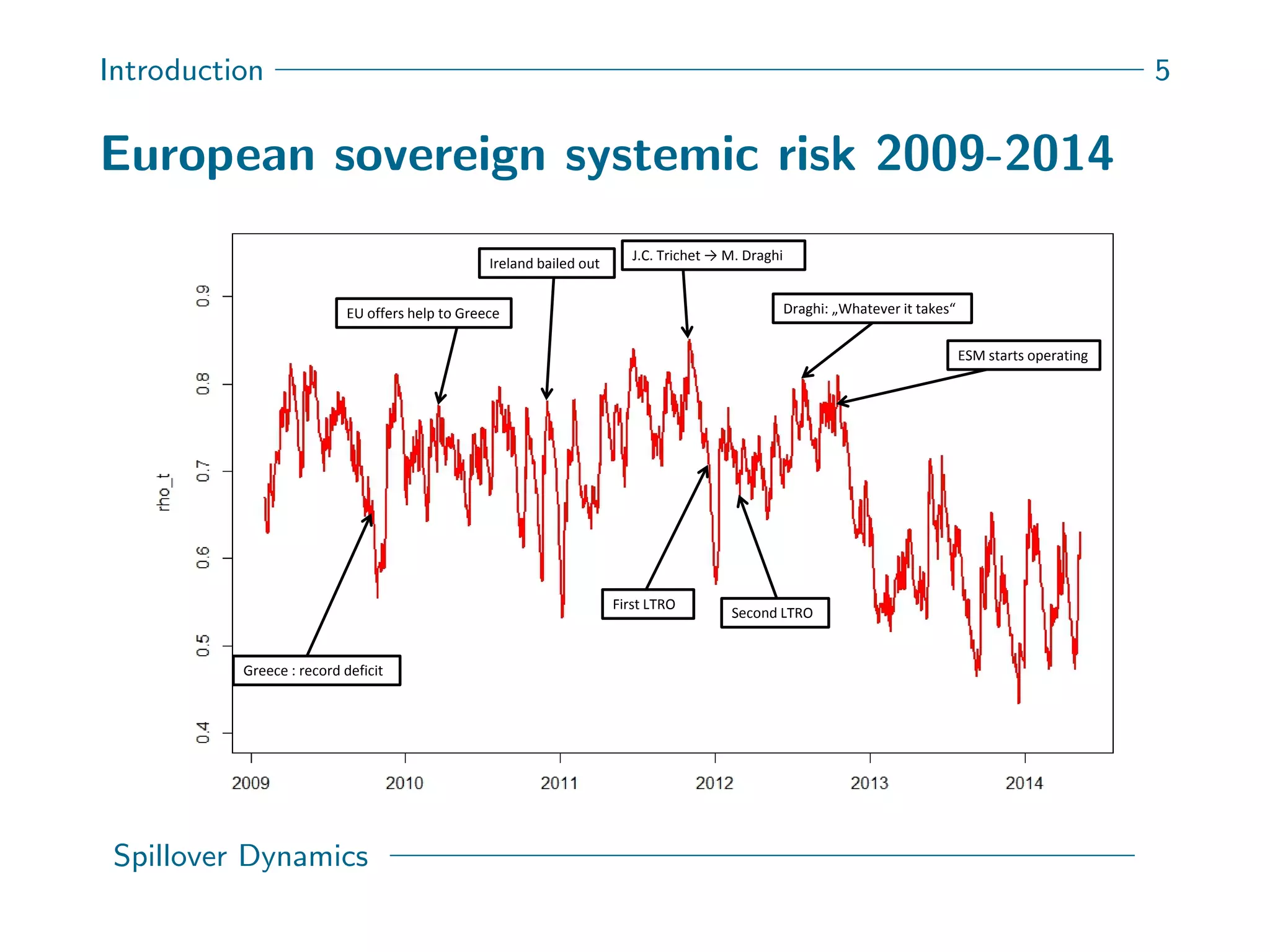
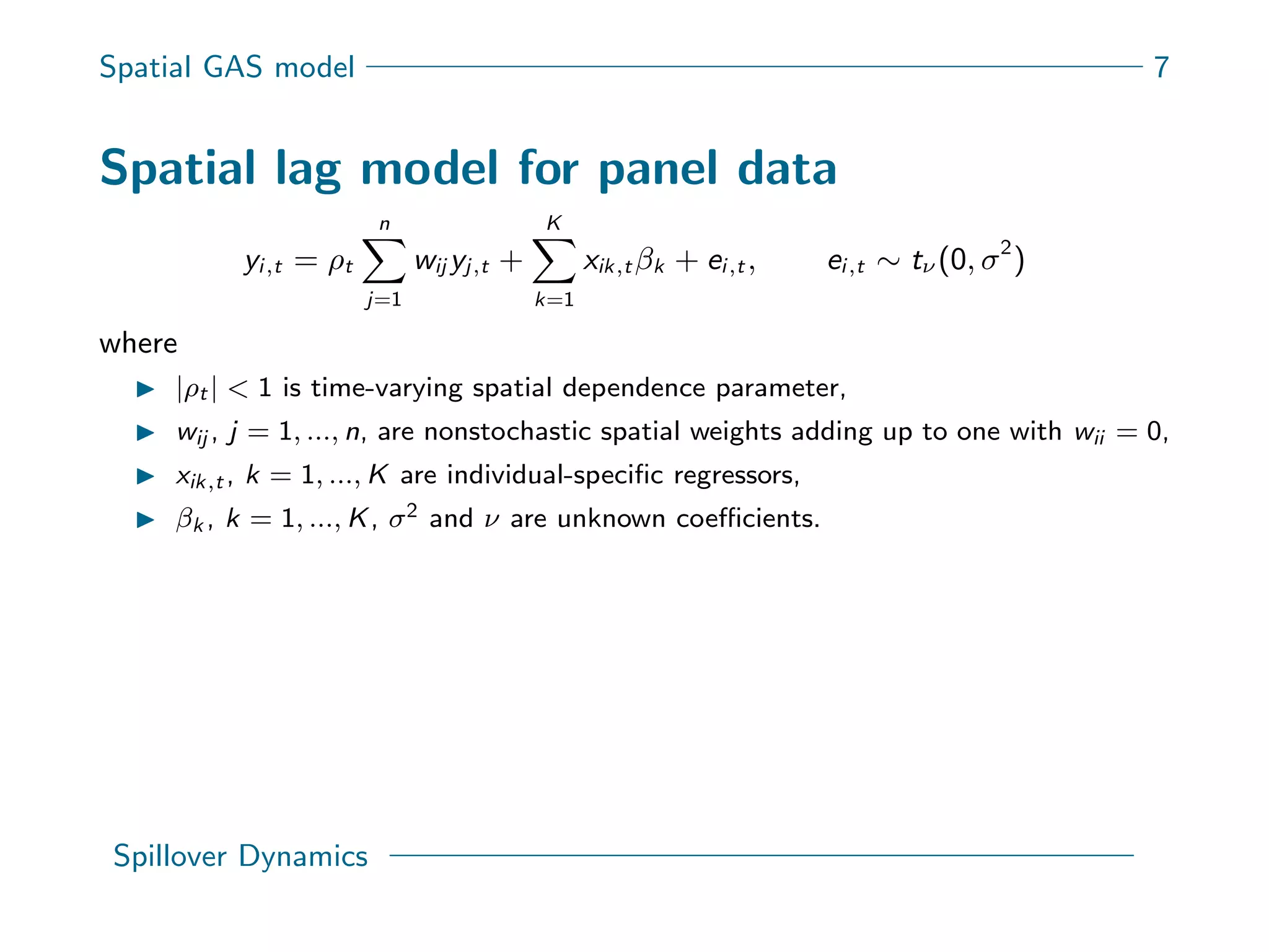
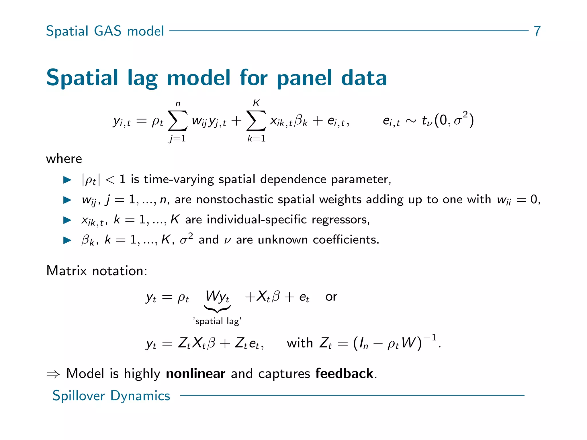
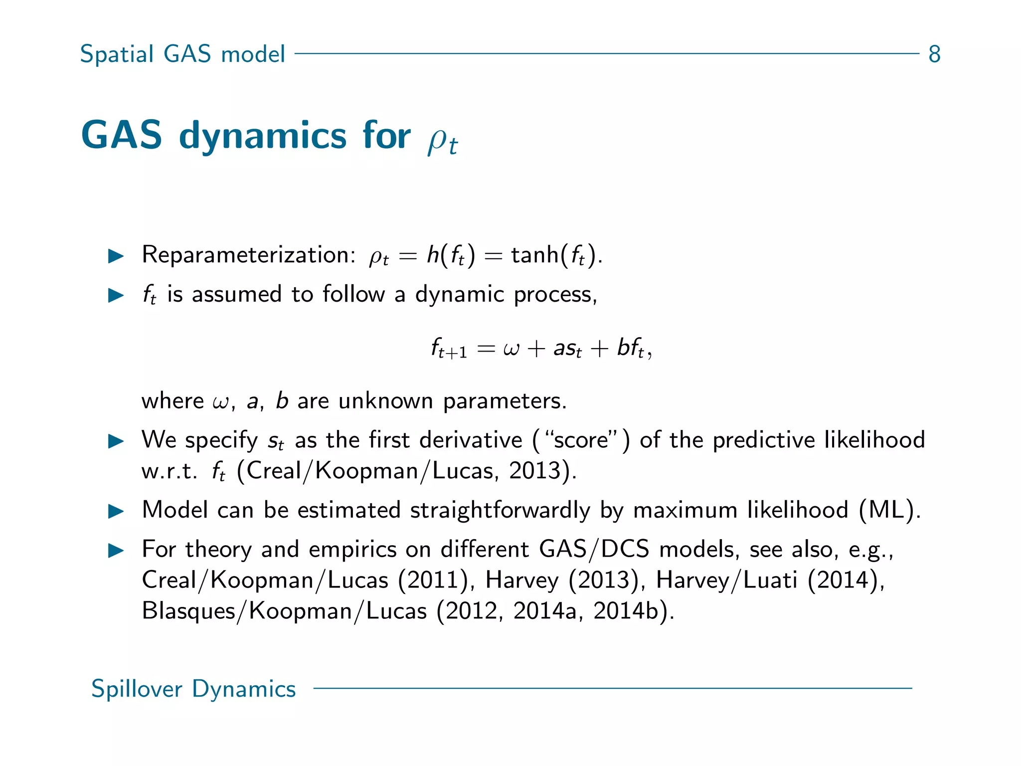
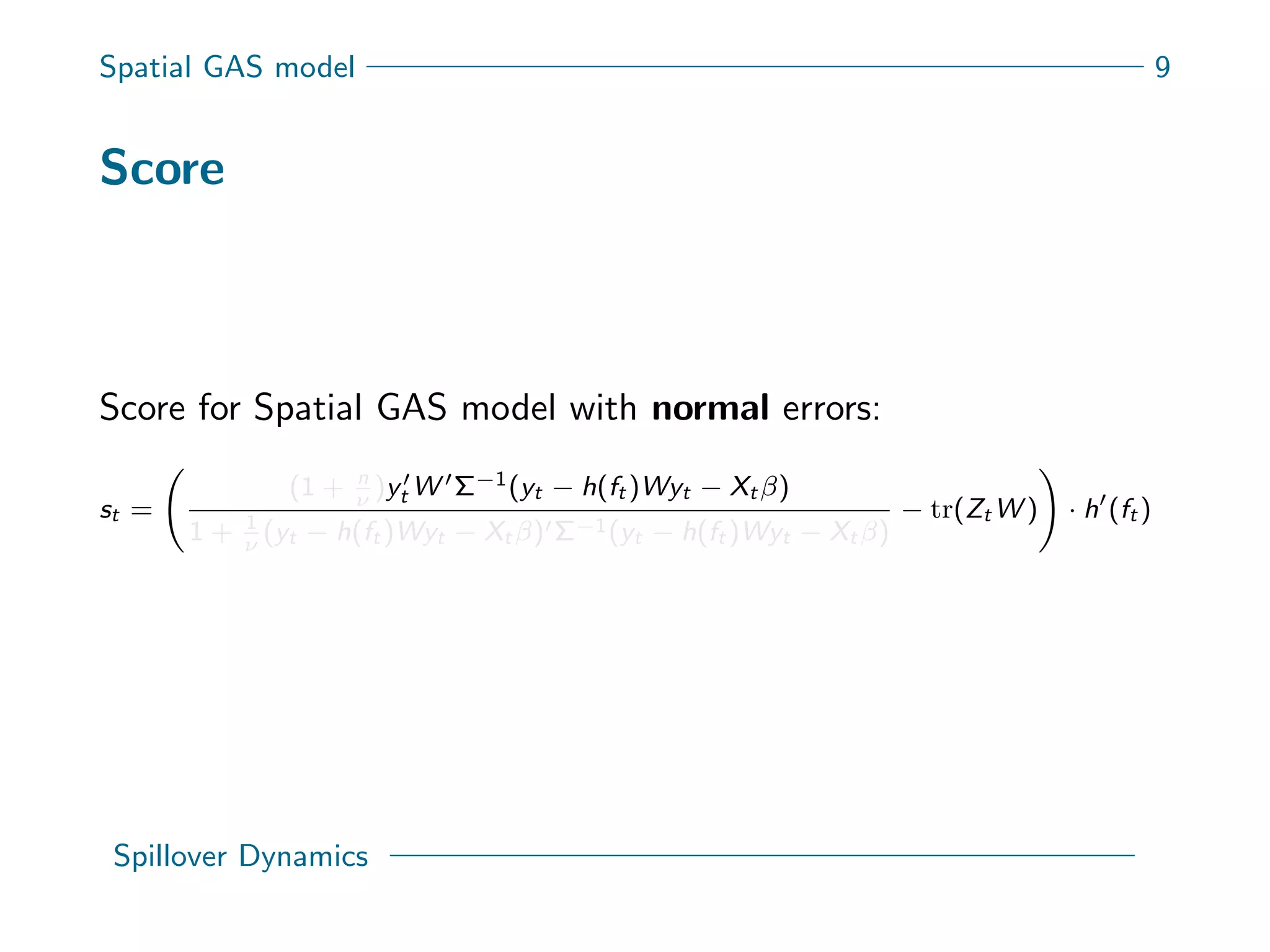
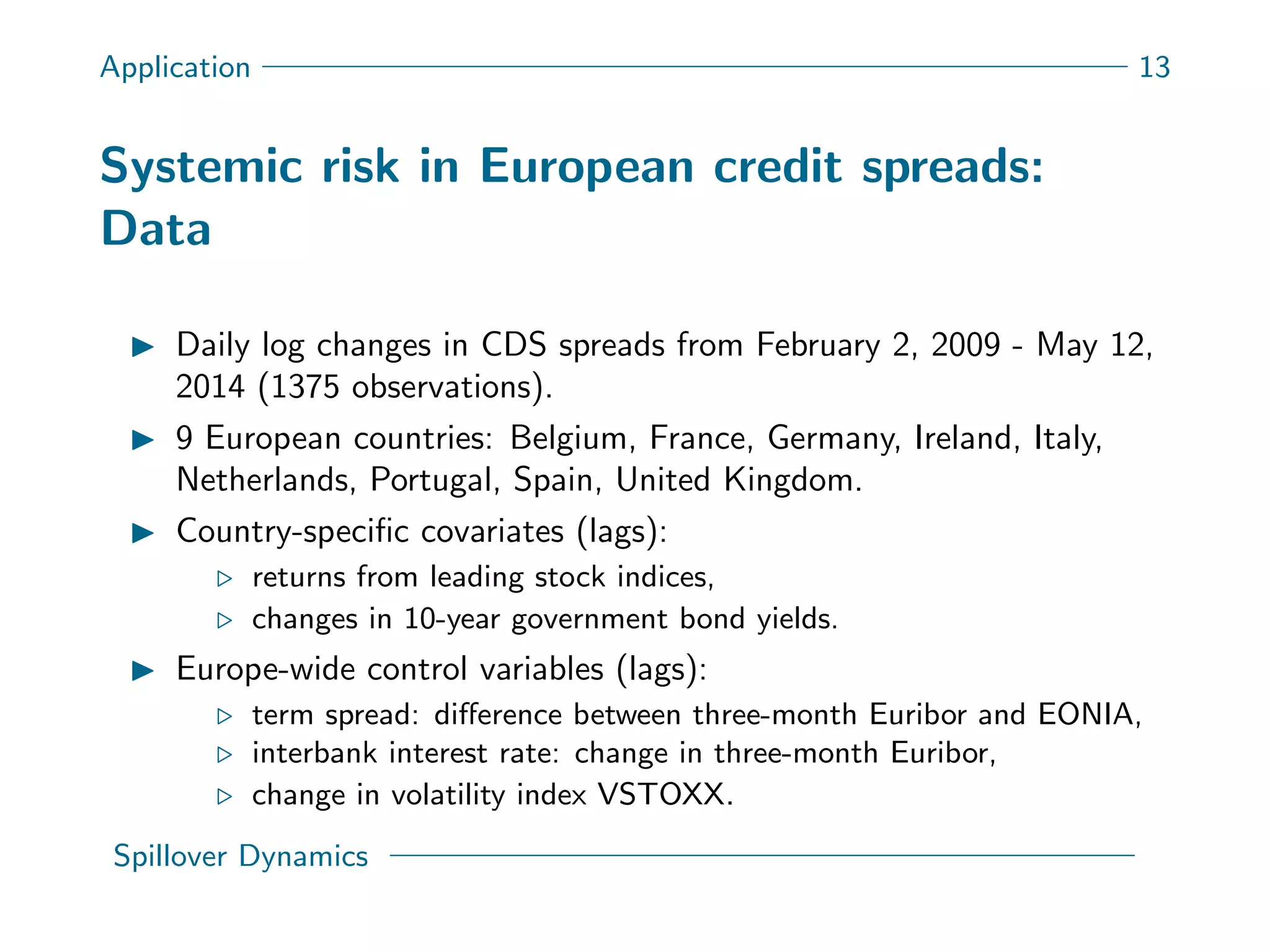
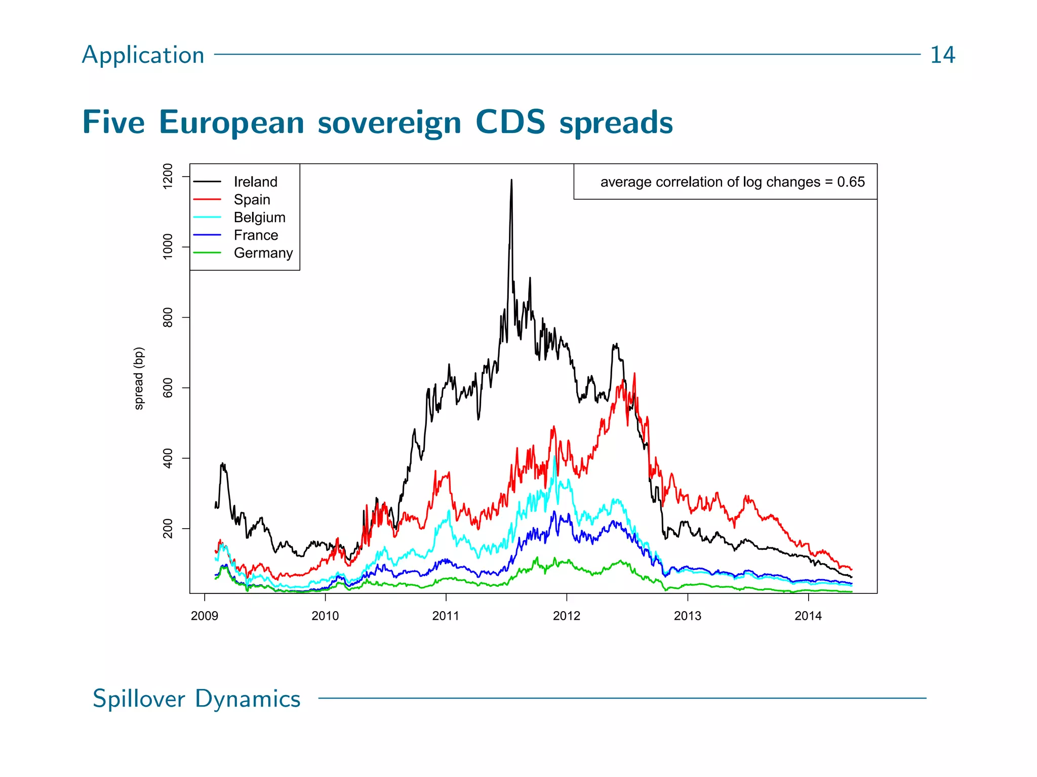
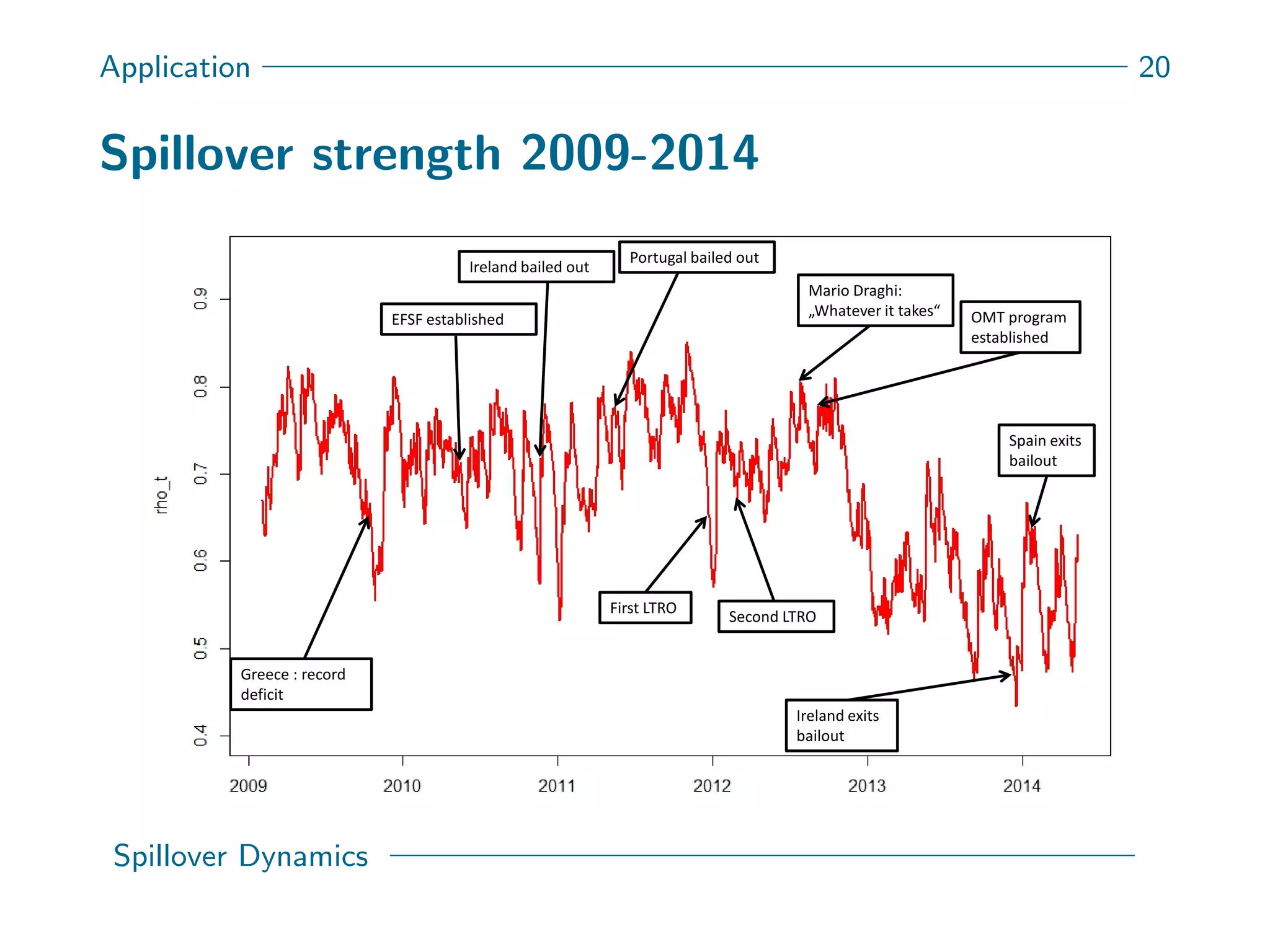
This document presents a new spatial gas model to measure systemic risk in European sovereign credit markets, focusing on spillover dynamics of credit spreads from 2009 to 2014. It incorporates time-varying parameters and fat tails to monitor the effects of policy interventions in the context of financial interconnectedness among European countries. The findings suggest a significant spatial dependence in credit risks and a decrease in systemic risk following government and ECB bailout measures.

1. Spillover Dynamics for Systemic
Risk Measurement Using Spatial
Financial Time Series Models
SYstemic Risk TOmography:
Signals, Measurements, Transmission Channels,
and Policy Interventions
FranciscoBlasques(a,b)
SiemJan Koopman(a,b,c)
AndreLucas(a,b,d)
JuliaSchaumburg(a,b)
(a)VU University Amsterdam (b)Tinbergen Institute (c)CREATES (d)Duisenberg School ofFinance
SeventhAnnualSoFiE Conference
Toronto,June 11-13,2014

2. This project has received funding from the European Union’s
Seventh Framework Programme for research, technological
development and demonstration under grant agreement no° 320270
www.syrtoproject.eu
This document reflects only the author’s views.
The European Union is not liable for any use that may be made of the information contained therein.

3. Introduction 3
Systemic sovereign credit risk
Systemic risk: Breakdown risk of the
financial system, induced by the
interdependence of its constituents.
Spillover Dynamics

4. Introduction 3
Systemic sovereign credit risk
Systemic risk: Breakdown risk of the
financial system, induced by the
interdependence of its constituents.
European sovereign debt since 2009:
Strong increases and comovements of credit spreads.
Financial interconnectedness across borders due to mutual
borrowing and lending + bailout engagements.
Spillover Dynamics

5. Introduction 3
Systemic sovereign credit risk
Systemic risk: Breakdown risk of the
financial system, induced by the
interdependence of its constituents.
European sovereign debt since 2009:
Strong increases and comovements of credit spreads.
Financial interconnectedness across borders due to mutual
borrowing and lending + bailout engagements.
⇒ Spillovers of shocks between member states.
⇒ Unstable environment: need for time-varying parameter models and
fat tails.
Spillover Dynamics

6. Introduction 4
This project
New parsimonious model for overall time-varying strength of
cross-sectional spillovers in credit spreads (systemic risk).
⇒ Useful for flexible monitoring of policy measure effects.
Extension of widely used spatial lag model to generalized
autoregressive score (GAS) dynamics and fat tails in financial data.
Asymptotic theory and assessment of finite sample performance of
this ’Spatial GAS model’.
Spillover Dynamics

7. Introduction 5
European sovereign systemic risk 2009-2014
Draghi: „Whatever it takes“
Ireland bailed out
EU offers help to Greece
J.C. Trichet → M. Draghi
First LTRO
Second LTRO
ESM starts operating
Greece : record deficit
Spillover Dynamics

8. Introduction 6
Some related literature
Systemic risk in sovereign credit markets:
Ang/Longstaff (2013), Lucas/Schwaab/Zhang (2013),
Aretzki/Candelon/Sy (2011), Kalbaska/Gatkowski (2012), De Santis
(2012), Caporin et al. (2014), Korte/Steffen (2013),
Kallestrup/Lando/Murgoci (2013), Beetsma et al. (2013, 2014).
Spatial econometrics:
General: Cliff/Ord (1973), Anselin (1988), Cressie (1993), LeSage/Pace
(2009), Ord (1975), Lee (2004), Elhorst (2003);
Panel data: Kelejian/Prucha (2010), Yu/de Jong/Lee (2008, 2012),
Baltagi et al. (2007, 2013), Kapoor/Kelejian/Prucha (2007);
Empirical finance: Keiler/Eder (2013), Fernandez (2011),
Asgarian/Hess/Liu (2013), Arnold/Stahlberg/Wied (2013), Wied (2012),
Denbee/Julliard/Li/Yuan (2013), Saldias (2013).
Spillover Dynamics

9. Spatial GAS model 7
Spatial lag model for panel data
yi,t = ρt
n
j=1
wij yj,t +
K
k=1
xik,t βk + ei,t , ei,t ∼ tν (0, σ2
)
where
|ρt | < 1 is time-varying spatial dependence parameter,
wij , j = 1, ..., n, are nonstochastic spatial weights adding up to one with wii = 0,
xik,t , k = 1, ..., K are individual-specific regressors,
βk , k = 1, ..., K, σ2 and ν are unknown coefficients.
Spillover Dynamics

10. Spatial GAS model 7
Spatial lag model for panel data
yi,t = ρt
n
j=1
wij yj,t +
K
k=1
xik,t βk + ei,t , ei,t ∼ tν (0, σ2
)
where
|ρt | < 1 is time-varying spatial dependence parameter,
wij , j = 1, ..., n, are nonstochastic spatial weights adding up to one with wii = 0,
xik,t , k = 1, ..., K are individual-specific regressors,
βk , k = 1, ..., K, σ2 and ν are unknown coefficients.
Matrix notation:
yt = ρt Wyt
’spatial lag’
+Xt β + et or
yt = Zt Xt β + Zt et , with Zt = (In − ρt W )−1
.
⇒ Model is highly nonlinear and captures feedback.
Spillover Dynamics

11. Spatial GAS model 8
GAS dynamics for ρt
Reparameterization: ρt = h(ft ) = tanh(ft ).
ft is assumed to follow a dynamic process,
ft+1 = ω + ast + bft ,
where ω, a, b are unknown parameters.
We specify st as the first derivative (“score”) of the predictive likelihood
w.r.t. ft (Creal/Koopman/Lucas, 2013).
Model can be estimated straightforwardly by maximum likelihood (ML).
For theory and empirics on different GAS/DCS models, see also, e.g.,
Creal/Koopman/Lucas (2011), Harvey (2013), Harvey/Luati (2014),
Blasques/Koopman/Lucas (2012, 2014a, 2014b).
Spillover Dynamics

12. Spatial GAS model 9
Score
Score for Spatial GAS model with normal errors:
st =
(1 + n
ν
)yt W Σ−1(yt − h(ft )Wyt − Xt β)
1 + 1
ν
(yt − h(ft )Wyt − Xt β) Σ−1(yt − h(ft )Wyt − Xt β)
− tr(Zt W ) · h (ft )
Spillover Dynamics

13. Spatial GAS model 10
Score
Score for Spatial GAS model with t-errors:
st =
(1 + n
ν
)yt W Σ−1(yt − h(ft )Wyt − Xt β)
1 + 1
ν
(yt − h(ft )Wyt − Xt β) Σ−1(yt − h(ft )Wyt − Xt β)
− tr(Zt W ) · h (ft )
Spillover Dynamics

14. Theory 11
Theory for Spatial GAS model
Extension of theoretical results on GAS models in
Blasques/Koopman/Lucas (2014a, 2014b).
Nonstandard due to nonlinearity of the model, particularly in the
case of Spatial GAS-t specification.
Conditions:
moment conditions;
b + a∂st
∂ft
is contracting on average.
Result: strong consistency and asymptotic normality of ML
estimator.
Also: Optimality results (see paper).
Spillover Dynamics

15. Simulation 12
Simulation results (n = 9, T = 500)
0 100 200 300 400 500
0.00.40.8
Sine, dense W, t−errorsrho.t
0 100 200 300 400 500
0.00.20.40.60.81.0
Step, dense W, t−errors
rho.t
Spillover Dynamics

16. Application 13
Systemic risk in European credit spreads:
Data
Daily log changes in CDS spreads from February 2, 2009 - May 12,
2014 (1375 observations).
9 European countries: Belgium, France, Germany, Ireland, Italy,
Netherlands, Portugal, Spain, United Kingdom.
Country-specific covariates (lags):
returns from leading stock indices,
changes in 10-year government bond yields.
Europe-wide control variables (lags):
term spread: difference between three-month Euribor and EONIA,
interbank interest rate: change in three-month Euribor,
change in volatility index VSTOXX.
Spillover Dynamics

17. Application 14
Five European sovereign CDS spreads
2009 2010 2011 2012 2013 2014
20040060080010001200
spread(bp)
Ireland
Spain
Belgium
France
Germany
average correlation of log changes = 0.65
Spillover Dynamics

18. Application 15
Spatial weights matrix
Idea: Sovereign credit risk spreads are (partly) driven by cross-border debt
interconnections of financial sectors (see, e.g. Korte/Steffen (2013),
Kallestrup et al. (2013)).
Intuition: European banks are not required to hold capital buffers against
EU member states’ debt (’zero risk weight’).
If sovereign credit risk materializes, banks become undercapitalized, so
that bailouts by domestic governments are likely, affecting their credit
quality.
Entries of W : Three categories (high - medium - low) of cross-border
exposures in 2008.∗
∗Source: Bank for International Settlements statistics, Table 9B: International
bank claims, consolidated - immediate borrower basis.
Spillover Dynamics

19. Application 16
Empirical model specifications
model mean equation errors et ∼
(0, σ2
In) (0, Σt)
Static spatial yt = ρWyt + Xtβ + et N, t
Sp. GAS yt = h(f ρ
t )Wyt + Xtβ + et N, t t
Sp. GAS+mean fct. yt = ZtXtβ + λf λ
t + Ztet t
Benchmark yt = Xtβ + λf λ
t + et t
Spillover Dynamics

20. Application 17
Model fit comparison
Static spatial Spatial GAS
et ∼ N(0, σ2In) tν (0, σ2In) N(0, σ2In) tν (0, σ2In)
logL -29614.62 -27623.06 -29460.51 -27546.63
AICc 59245.35 55264.24 58941.19 55115.45
Spatial GAS-t Benchmark-t
(+tv. volas) (+mean f.+tv.volas) (+mean f.+tv.volas)
logL -27174.94 -27153.83 -30161.63
AICc 54392.57 54354.47 60384.65
Spillover Dynamics

21. Application 18
Parameter estimates
Spatial dependence is high and significant.
Spatial GAS parameters:
High persistence of dynamic factors reflected by large
estimates for b.
Estimates for score impact parameters a are small but
significant.
Estimates for β have expected signs.
Mean factor loadings:
Positive for Ireland, Italy, Portugal, Spain.
Negative for Belgium, France, Germany, Netherlands.
Spillover Dynamics

22. Application 19
Different choices of W
Candidates (all row-normalized):
Raw exposure data (constant): Wraw
Raw exposure data (updated quarterly): Wdyn
Three categories of exposure amounts (high, medium, low): Wcat
Exposures standardized by GDP: Wgdp
Geographical neighborhood (binary, symmetric): Wgeo
Spillover Dynamics

23. Application 19
Different choices of W
Candidates (all row-normalized):
Raw exposure data (constant): Wraw
Raw exposure data (updated quarterly): Wdyn
Three categories of exposure amounts (high, medium, low): Wcat
Exposures standardized by GDP: Wgdp
Geographical neighborhood (binary, symmetric): Wgeo
Model fit comparison (only t-GAS model):
Wraw Wdyn Wcat Wgdp Wgeo
logL 27973.02 -27946.97 -27153.83 -27992.69 -28890.98
Parameter estimates are robust.
Spillover Dynamics

24. Application 20
Spillover strength 2009-2014
Mario Draghi:
„Whatever it takes“
Ireland bailed out
EFSF established
Portugal bailed out
First LTRO
Second LTRO
OMT program
established
Greece : record
deficit
Ireland exits
bailout
Spain exits
bailout
Spillover Dynamics

25. Conclusions 21
Conclusions
Spatial model with dynamic spillover strength and fat tails is
new, and it works (theory, simulation, empirics).
European sovereign CDS spreads are strongly spatially
dependent.
Decrease of systemic risk from mid-2012 onwards; possibly
due to EU governments’ and ECB’s bailout measures.
Best model: Time-varying spatial dependence based on
t-distributed errors, time-varying volatilities, additional mean
factor, and categorical spatial weights.
Spillover Dynamics

26. Thank you.