This document provides an overview of key principles of actuarial science including traditional applications in insurance, probability basics, common probability distributions used in actuarial science like Poisson and binomial, and concepts like expectation, variance, and moments. It also gives examples of calculating probabilities and parameters for Poisson and binomial distributions.

1. 1
Week 1 1
Principles of Actuarial Science;
Games of Chance (1)
Outline:
1. Traditional Actuarial Application: Insurance
2. Principles of Actuarial Science
3. Probability Basics (Revision?)
4. Poisson and Binomial Distributions
Reading
(Req) Sherris, 1.3-1.4, 2.1-2.3
(Recc) Sherris 1.1-1.2
1
Version: 15 July 2010. Copyright UNSW Actuarial Studies

2. 2
Traditional Application of Actuarial Science - Insurance
What is insurance?
Examples:
– Life (Death)
– Life (Survival)
– Health
– Disability
– Motor
– House
– Home Contents
– Workers Compensation
Fundamental Idea: Payment(s) that are incurred when a (random) event occurs
Other actuarial applications: Superannuation, Risk Management
(Will discuss in much more detail later in the course)

3. 3
Discussion
Consider a life insurance policy that:
– pays $100 at the end of the year if the policyholder ("Harry P") dies during the year
– assume that Harry has a 50% chance of dying
Q: Suppose that you are the actuary of the insurance company. Suggest how you
would determine the premium of this policy (making any additional assumptions if
required)

4. 4
Basic Principles of Actuarial Science
Probability and Statistics
– quantify future uncertainty
– probability models - Binomial, Poisson, Normal, Log-Normal
– Survival models
Risk Pooling
– Independent Risks
– Risk Factors (age, sex, smoker status etc)
Law of Large Numbers
– Expected values
– Variability of averages less for pools of independent risks

5. 5
Interest Rates
– Time Value of money
– economics of interest rates
– present values
Risk
– Utility Theory and Ranking of risky outcomes
– expected utility principle, certainty equivalents

6. 6
Discussion (ctd)
Suppose the premium for the policy has been set at $55, and that interest rates are
0.
What are some of the practical issues the company must now consider? Consider:
–(i) What to do with the $55 received as a premium?
(ii) How should this policy be reflected in the company’s financial reports?

7. 7
Basic Principles of Actuarial Science (ctd)
Financial Principles
– Accounting and Market values
– Fair Value of Liabilities
Actuarial Modelling
– Contingent Cash flows
– Death, survival, illness, financial asset returns

8. 8
Risk Management
– What is risk?
– Pooling and Diversification of Risk
– Experience Rating
– Profit Sharing
– Solvency
Risk Classification
– Moral Hazard
Careless or deliberate actions of insured affect payments
– Adverse Selection
Worse than average risks have incentives to purchase insurance
– Information Asymmetry

9. 9
Probability and Games of Chance
Probability
Permutation and Combinations
Useful Result: Binomial Theorem:
(x + y)n
=
n
X
r=0
n
r
xn r
yr
Simple method of determining probabilities (where/if possible!):
– Evaluate all possible equally likely cases
– Count the Frequency or proportion of times that the event occurs

10. 10
Example
What is the probability of rolling a total of 12 with three dice?

11. 11
Sum Frequency
3 1
4 3
5 6
6 10
7 15
8 21
9 25
10 27
11 27
12 25
13 21
14 15
15 10
16 6
17 3
18 1
Total 216

12. 12
Random Variables
A random variable X is a function that assigns values to possible outcomes.
Discrete random variables - fixed number of finite values or countably infinite possible
values.
Continuous random variables - values on a continuous scale
Examples in Actuarial Science:
– Number of motor vehicle accidents occurring during a particular month
– Number of lives who die from cancer who are aged 40 last birthday during a par-
ticular time period.
– Time until the first accident for a particular car insurance policy
– Claim payment for a fire insurance policy

13. 13
Probability Density and Distribution Functions
Probability a discrete random variable X takes a particular value x is denoted
f(x) = P(X = x)
Probability density has the properties
f(x) 0 and
X
all x
f(x) = 1
Distribution function, (= "cumulative distribution function") of X; is the probability that
the random variable takes a value less than or equal to a specified value x
F(x) = Pr (X x)

14. 14
For continuous random variables the probability density function (p.d.f.) f(x) is de-
fined such that
Pr (a X b) =
Z b
a
f(x)dx
with
f(x) 0 for 1 < x < 1
Z 1
1
f(t)dt = 1
CDF:
F(x) = Pr (X x)
=
Z x
1
f(t)dt

15. 15
Expectation
Discrete random variable - expectation of a function of a random variable g(X) is
defined as
E [g (X)] =
X
all x
g (x) f(x)
Continuous random variable
E [g (X)] =
Z 1
1
g (x) f(x)dx

16. 16
Moments
Moments (about the origin) of a random variable are defined as
E [Xr
] r = 1; 2; : : :
First moment (r = 1) is the mean of the distribution of the random variable - usually
denoted by .
Discrete random variable
E [X] = =
X
all x
xf(x)
Continuous random variable
E [X] = =
Z 1
1
xf(x)dx

17. 17
Moments - Variance
The mean is a measure of central tendency for a distribution.
The second moment about the mean is referred to as the variance of the distribution.
Variance usually denoted by 2
V ar [X] = 2
= E
h
(X )2
i
The standard deviation is the square root of the variance, .
The variance is a measure of dispersion or spread of the distribution.

18. 18
Example
Consider a random variable X which takes the value 1 if Harry P dies and 0 if he
survives the year.. Find the mean, variance and standard deviation of X:

19. 19
Common Distributions in Actuarial Science
Poisson
Binomial
Geometric
Exponential
Normal
Log-Normal
Weibull

20. 20
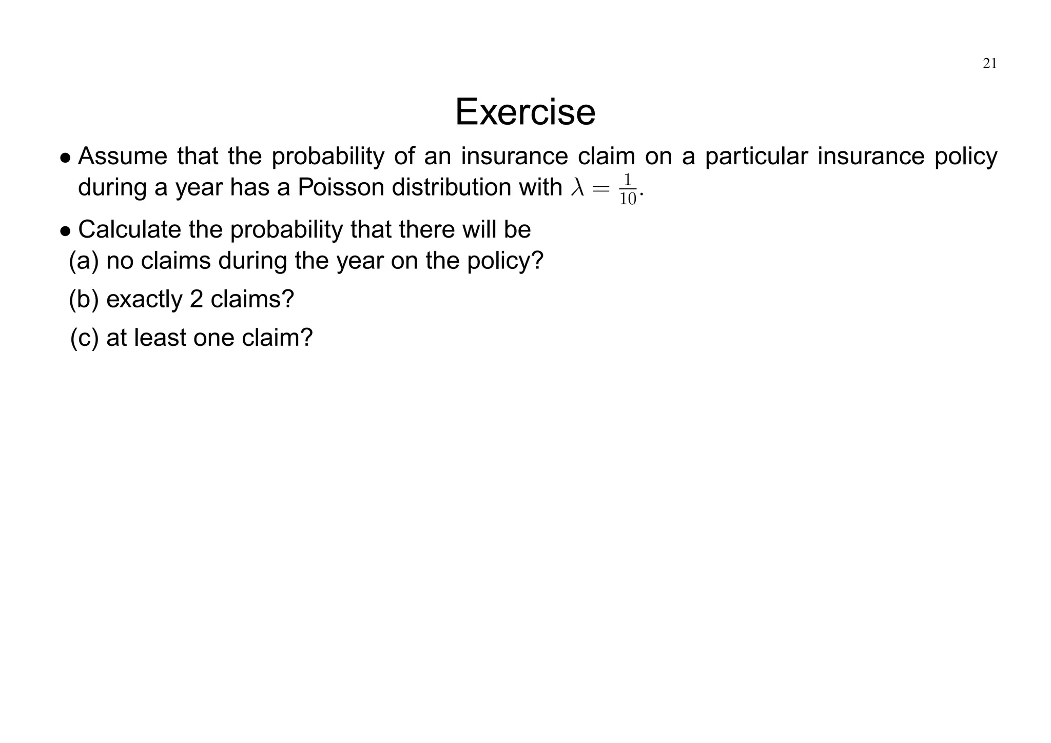
Poisson Distribution
The Poisson distribution
- often used to model the probability of occurrence of rare events such as insurance
claims
- also as an approximation for the chance of dying for a small enough parameter .
Poisson ( )
Pr (X = x) =
e x
x!
x = 0; 1; 2 : : :
E [X] =
V ar [X] =

21. 21
Exercise
Assume that the probability of an insurance claim on a particular insurance policy
during a year has a Poisson distribution with = 1
10:
Calculate the probability that there will be
(a) no claims during the year on the policy?
(b) exactly 2 claims?
(c) at least one claim?

22. 22
Binomial Distribution
Number of successes (x) in a series of n independent trials where each success has
probability p.
In actuarial science
– probability that a number of lives in a group of lives with the same chance of dying
will die assuming independence between the lives.
Binomial (n; p)
Pr (X = x) =
n
x
px
(1 p)n x
x = 0; 1; 2 : : :
E [X] = np
V ar [X] = np (1 p)

23. 23
Example
Suppose we have 100 policyholders, each with a probability of 0.2 of dying within the
next year. What is the probability that we observe a total of 10 or less deaths by the
end of the year?