1
Chapter 2: Single-Stage Simple Random Sampling
After a target population is defined and decision is made to use sample survey as a method of data
collection, there are several methods of statistical sampling techniques to use for the intended purpose.
These include simple random sampling, stratified random sampling, systematic sampling, cluster
sampling and multi-stage sampling. All of these techniques have one sampling characteristic in
common. Each deals with a method of random sample selection from a defined target population to be
investigated. The random selection procedure ensures that each population unit has an equal chance of
being included in the sample. It is this random selection method that provides representative samples
impartially and without bias by avoiding any influence of human being. Each technique will be
discussed in subsequent chapters.
This chapter will present the basic principles and characteristics of single-stage simple random
sampling technique. Simple random sampling is very important as a basis for development of the
theory of sampling. It serves as a central reference for all other sampling designs.
2.1 Definition and Basic Concepts
Simple random sampling (SRS) is a basic probability sampling selection technique in which a
predetermined number of sample units are selected from a population list (sampling frame) so that
each unit on the list has an equal chance of being included in the sample. Simple random sampling also
makes the selection of every possible combination of the desired number of units equally likely. In this
way, each sample has an equal chance of being selected. If the population has N units then a random
method of selection is one which gives each of the N units in the population to be covered a calculable
probability of being selected.
To undertake a sample selection, there are two types of random sampling selection−sampling with
replacement (wr) and sampling without replacement (w o r).
Sampling Without Replacement:
Sampling without replacement (wor) means that once a unit has been selected, it cannot be selected
again. In other words, it means that no unit can appear more than once in the sample. If there are n
sample units required for selection from a population having N units, then there are 







n
N
ways of
selecting n units out of a total of N units without replacement, disregarding the order of the n units.
Hence, simple random sampling is equivalent to the selection of one of the 







n
N
possible samples with
an equal probability 







n
N
1 assigned to each sample.
In simple random sampling without replacement the probability of a specified unit of the population
being selected at any given draw is equal to the probability of its being selected at the first draw, that
is, N
1 . However, for a sample of size n, the sum of the probabilities of these mutually exclusive
events is N
n .
Sampling with replacement:
2
The process of sampling with replacement (wr) allows for a unit to be selected on more than one draw.
There are Nn
ways of selecting n units out of a total of N units with replacement. In this case, the order
of selection will be considered. All selections are independent since the selected unit is returned to the
population before making the next selection. Thus, the probability is N
1 for any specific element on
each of the n draws.
Simple random sampling with or without replacement is practically identical if the sample size is a
very small fraction of the population size. Generally, sampling without replacement yields more
precise results and is operationally more convenient.
2.2 Simple Random Sample Selection Procedures
In sample survey when sample units are selected from a population there could be possibilities of
biases in the selection procedure which may come from the use of a non-random method. That is, the
selection is consciously or unconsciously influenced by subjective judgment of human being. Such
bias can be avoided by using a random selection method. The true randomness can be ensured by using
the method of selection which cannot be affected by human influence.
There are different random sample selection methods. The important aspect of random selection in
each method is that the selection of each unit is based purely on chance. This chance is known as
probability of selection which eliminates selection bias. If there is a bias in the selection, it may
prevent the sample from being representative of the population. Representative means that probability
samples permits scientific approaches in which the samples give accurate estimates of the total
population. We consider here two basic and common procedures of random selection method.
Lottery Method:
This is a very common method of taking a random sample. Under this method, we label each member
of the population by identifiable disc or a ticket or pieces of paper. Discs or tickets must be of identical
size, color and shape. They are placed in a container (urn/bowl) and well mixed before each draw, and
then without looking into the container selection of designated labels will be performed with or
without replacement. Then series of drawing may be continued until a sample of the required size is
selected. This procedure shows that selection of each item depends entirely on chance.
For example, if we want to take a sample of 18 persons out of a population of 90 persons, the
procedure is to write the names of all the 90 persons on separate slips (tickets) of paper. The slips
(tickets) of paper must be of identical size, color and shape. The next step is to fold these slips, mix
them thoroughly and then make a blindfold selection of 18 slips one at a time without replacement.
This lottery method becomes quite cumbersome and time consuming to use as the sizes of sample and
population increase. To avoid such problems and to reduce the labor of selection process, another
method known as a random number table selection process can be used.
The Use of Random Numbers:
A table of random numbers consists of digits from 0 to 9, which are equally represented with no
pattern or order, produced by a computer random number generator. The members of the population
are numbered from 1 to N and n numbers are selected from one of the random tables in any convenient
and systematic way. The procedure of selection is outlined as follows.
3
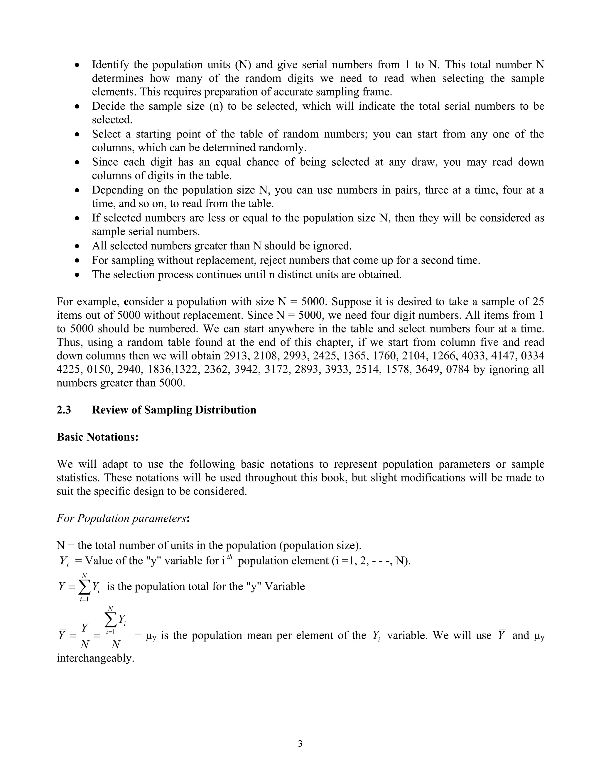
• Identify the population units (N) and give serial numbers from 1 to N. This total number N
determines how many of the random digits we need to read when selecting the sample
elements. This requires preparation of accurate sampling frame.
• Decide the sample size (n) to be selected, which will indicate the total serial numbers to be
selected.
• Select a starting point of the table of random numbers; you can start from any one of the
columns, which can be determined randomly.
• Since each digit has an equal chance of being selected at any draw, you may read down
columns of digits in the table.
• Depending on the population size N, you can use numbers in pairs, three at a time, four at a
time, and so on, to read from the table.
• If selected numbers are less or equal to the population size N, then they will be considered as
sample serial numbers.
• All selected numbers greater than N should be ignored.
• For sampling without replacement, reject numbers that come up for a second time.
• The selection process continues until n distinct units are obtained.
For example, consider a population with size N = 5000. Suppose it is desired to take a sample of 25
items out of 5000 without replacement. Since N = 5000, we need four digit numbers. All items from 1
to 5000 should be numbered. We can start anywhere in the table and select numbers four at a time.
Thus, using a random table found at the end of this chapter, if we start from column five and read
down columns then we will obtain 2913, 2108, 2993, 2425, 1365, 1760, 2104, 1266, 4033, 4147, 0334
4225, 0150, 2940, 1836,1322, 2362, 3942, 3172, 2893, 3933, 2514, 1578, 3649, 0784 by ignoring all
numbers greater than 5000.
2.3 Review of Sampling Distribution
Basic Notations:
We will adapt to use the following basic notations to represent population parameters or sample
statistics. These notations will be used throughout this book, but slight modifications will be made to
suit the specific design to be considered.
For Population parameters:
N = the total number of units in the population (population size).
i
Y = Value of the "y" variable for i th
population element (i =1, 2, - - -, N).

=
=
N
i
i
Y
Y
1
is the population total for the "y" Variable
N
Y
N
Y
Y
N
i
i

=
=
= 1
= y is the population mean per element of the i
Y variable. We will use Y and y
interchangeably.
4
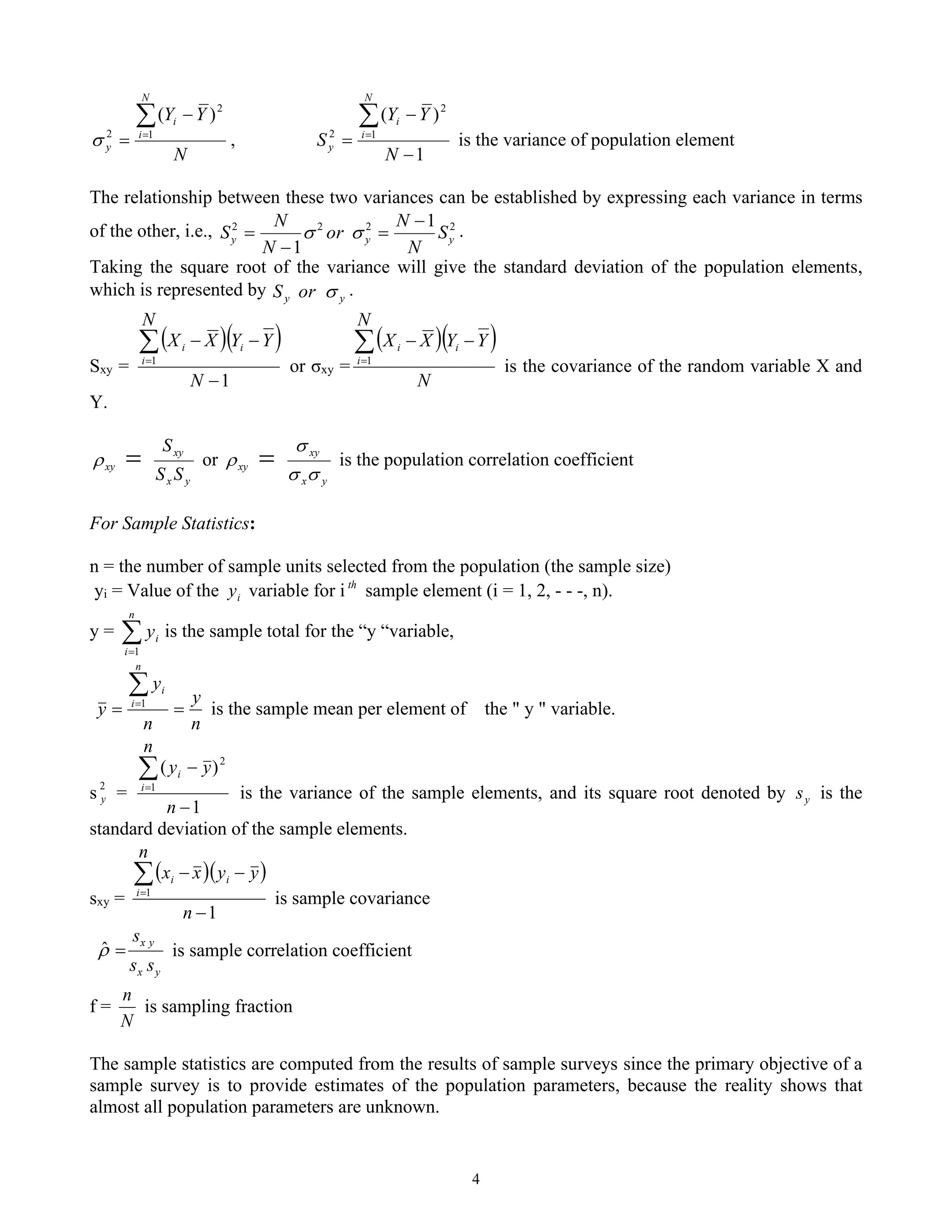
N
Y
Y
N
i
i
y

=
−
= 1
2
2
)
(
 ,
1
)
(
1
2
2
−
−
=

=
N
Y
Y
S
N
i
i
y is the variance of population element
The relationship between these two variances can be established by expressing each variance in terms
of the other, i.e., 2
2
2
2 1
1
y
y
y S
N
N
or
N
N
S
−
=
−
= 
 .
Taking the square root of the variance will give the standard deviation of the population elements,
which is represented by y
y or
S  .
Sxy =
( )( )
1
1
−
−
−

=
N
Y
Y
N
X
X i
i
i
or σxy =
( )( )
N
Y
Y
N
X
X i
i
i −
−

=1
is the covariance of the random variable X and
Y.
y
x
xy
xy
S
S
S
=
 or
y
x
xy
xy



 = is the population correlation coefficient
For Sample Statistics:
n = the number of sample units selected from the population (the sample size)
yi = Value of the i
y variable for i th
sample element (i = 1, 2, - - -, n).
y = 
=
n
i
i
y
1
is the sample total for the “y “variable,
n
y
n
y
y
n
i
i
=
=

=1
is the sample mean per element of the " y " variable.
s 2
y =
1
)
(
1
2
−
−

=
n
n
y
y
i
i
is the variance of the sample elements, and its square root denoted by y
s is the
standard deviation of the sample elements.
sxy =
( )( )
1
1
−
−
−

=
n
y
y
n
x
x i
i
i
is sample covariance
y
x
y
x
s
s
s
=
̂ is sample correlation coefficient
f =
N
n
is sampling fraction
The sample statistics are computed from the results of sample surveys since the primary objective of a
sample survey is to provide estimates of the population parameters, because the reality shows that
almost all population parameters are unknown.
5
Sampling Variability
The sample statistics, calculated from selected sample units, are subject to sampling variability. They
depend on the number of sample units (sample size) and types of units included in the sample. Each
unit in the population has different characteristic and/or value. For example, a salary of employees
varies from individuals to individuals in which the magnitude of salary to be used in the calculation of
average income depends on the types of employees selected from the totals workers. Similarly the
number of sample workers selected (sample size) will affect the sample values. This indicates that the
sample statistics such as mean, total, variance, ratio and proportion are random variables. Like other
random variables, these sample statistics possess a probability distribution, which is more commonly
known as sampling distribution.
Sampling Distribution:
What is sampling distribution? What is the purpose of computing sampling distribution? The following
example will illustrate the basic idea of sampling distribution and its use.
Example 2.1:
For demonstration purpose we will consider a very small hypothetical population of 5 farmers, who
use fertilizer in their farming. Suppose the amount of fertilizer used (in kg) by each farmer is 70, 78,
80, 80, and 95. Then, the following parameters of the population and sample values (statistics) are
computed to justify the basic idea behind estimation.
Population Parameters:
Let i
Y denotes the amount of fertilizer used by each farmer (i =1, 2, - - -, 5). The population size is 5,
i.e. N = 5. The total amount of fertilizer used by all farmers and the average fertilizer consumption per
farmer are computed as follows.
The total amount of fertilizer used is 
=
=
N
i
i
Y
Y
1
= 70 + 78 + 80 + 80 + 95 = 403 kg.
The mean consumption of fertilizer per farmer is
N
Y
Y = = =
5
403
80.6 kg.
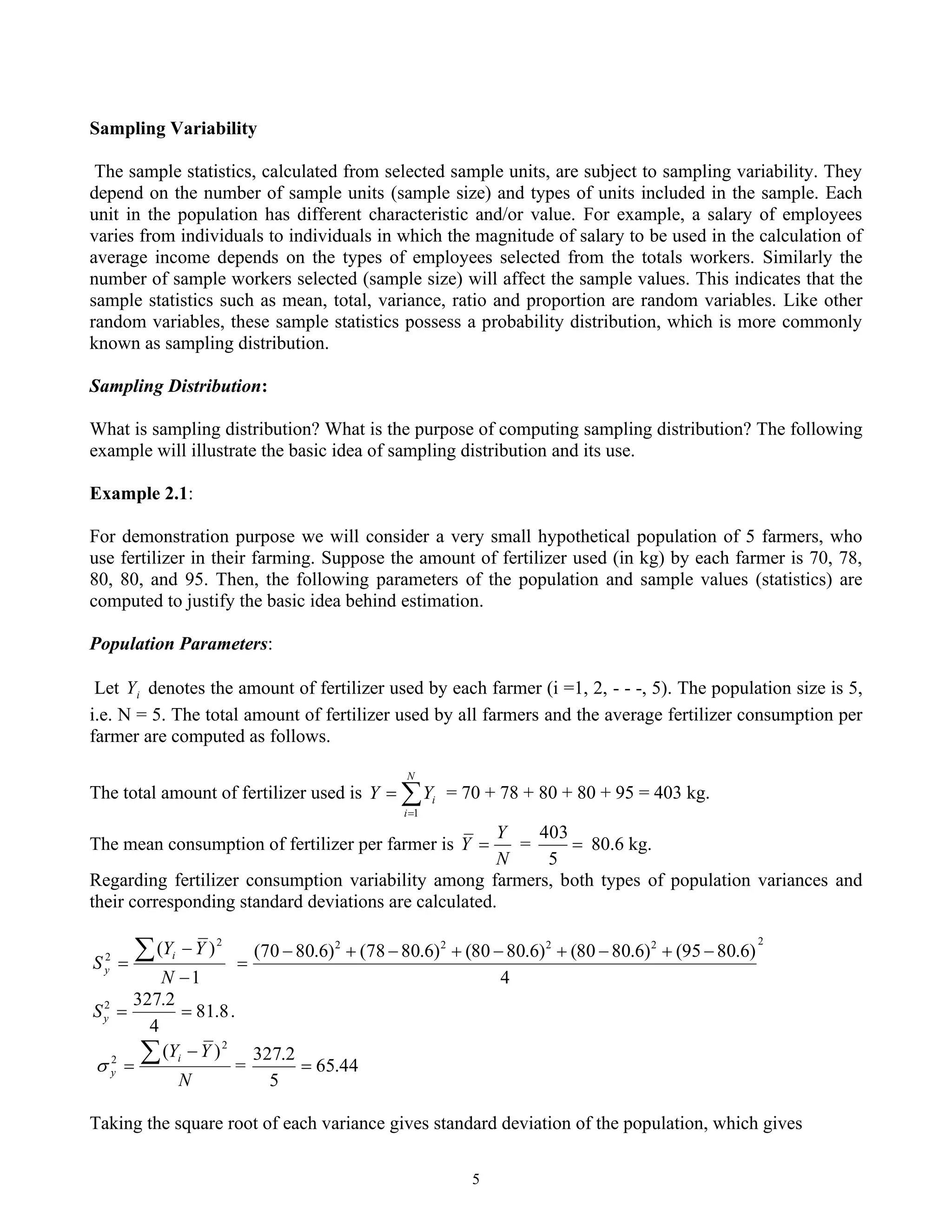
Regarding fertilizer consumption variability among farmers, both types of population variances and
their corresponding standard deviations are calculated.
1
)
( 2
2
−
−
=

N
Y
Y
S
i
y
2
2
2
2
2
4
)
6
.
80
95
(
)
6
.
80
80
(
)
6
.
80
80
(
)
6
.
80
78
(
)
6
.
80
70
( −
+
−
+
−
+
−
+
−
=
8
.
81
4
2
.
327
2
=
=
y
S .
N
Y
Yi
y
 −
=
2
2
)
(
 = 44
.
65
5
2
.
327
=
Taking the square root of each variance gives standard deviation of the population, which gives
6
S y = 9.044, and 089
.
8
=
Y
 . In reality all these population characteristics are mostly unknown for
relatively large size of population and should be estimated from survey results collected and
summarized from sample elements.
Now we want to estimate these population values from sample elements assuming that population
parameters are unknown. In the following sampling distribution we will examine all possible samples.
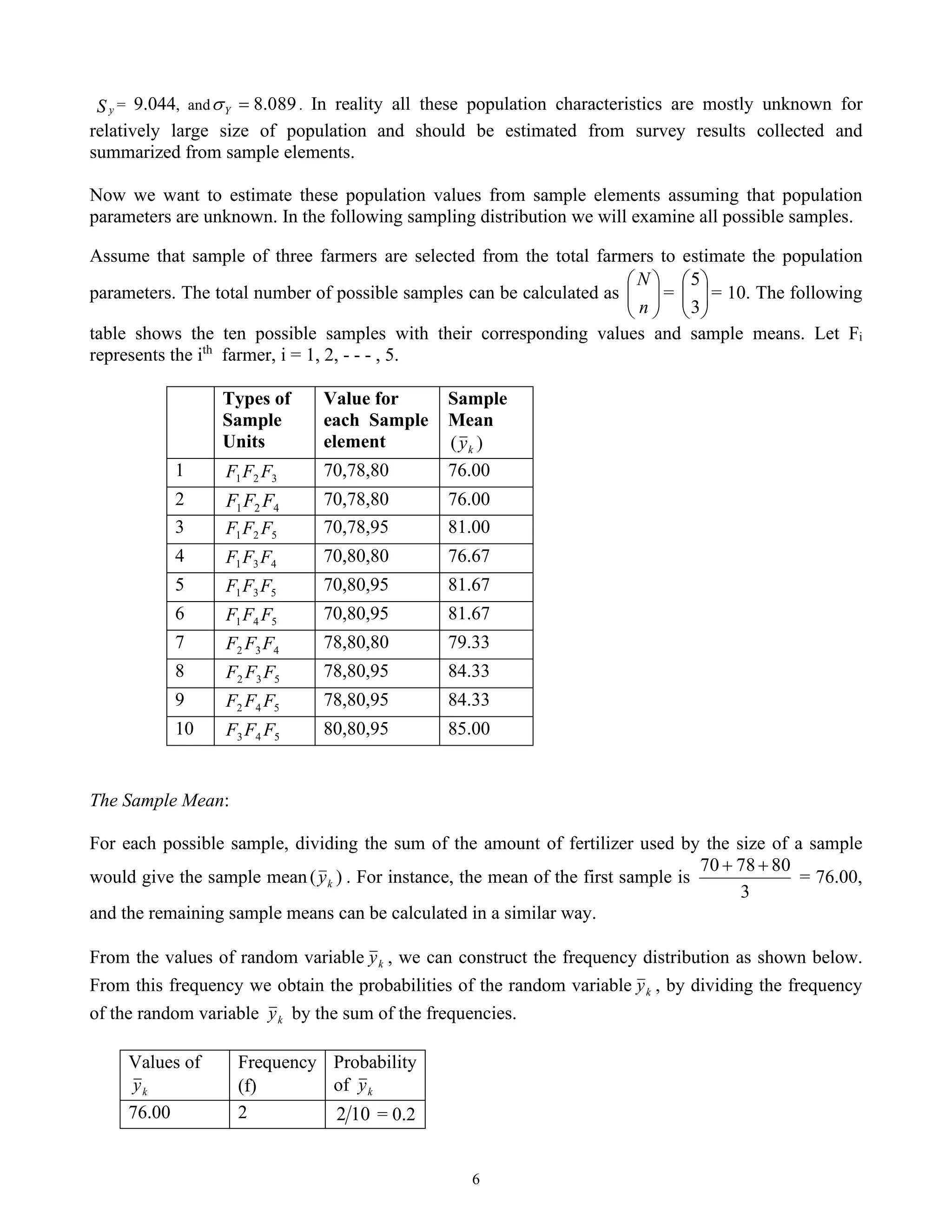
Assume that sample of three farmers are selected from the total farmers to estimate the population
parameters. The total number of possible samples can be calculated as 







n
N
= 







3
5
= 10. The following
table shows the ten possible samples with their corresponding values and sample means. Let Fi
represents the ith
farmer, i = 1, 2, - - - , 5.
Types of
Sample
Units
Value for
each Sample
element
Sample
Mean
)
( k
y
1 3
2
1 F
F
F 70,78,80 76.00
2 4
2
1 F
F
F 70,78,80 76.00
3 5
2
1 F
F
F 70,78,95 81.00
4 4
3
1 F
F
F 70,80,80 76.67
5 5
3
1 F
F
F 70,80,95 81.67
6 5
4
1 F
F
F 70,80,95 81.67
7 4
3
2 F
F
F 78,80,80 79.33
8 5
3
2 F
F
F 78,80,95 84.33
9 5
4
2 F
F
F 78,80,95 84.33
10 5
4
3 F
F
F 80,80,95 85.00
The Sample Mean:
For each possible sample, dividing the sum of the amount of fertilizer used by the size of a sample
would give the sample mean )
( k
y . For instance, the mean of the first sample is
3
80
78
70 +
+
= 76.00,
and the remaining sample means can be calculated in a similar way.
From the values of random variable k
y , we can construct the frequency distribution as shown below.
From this frequency we obtain the probabilities of the random variable k
y , by dividing the frequency
of the random variable k
y by the sum of the frequencies.
Values of
k
y
Frequency
(f)
Probability
of k
y
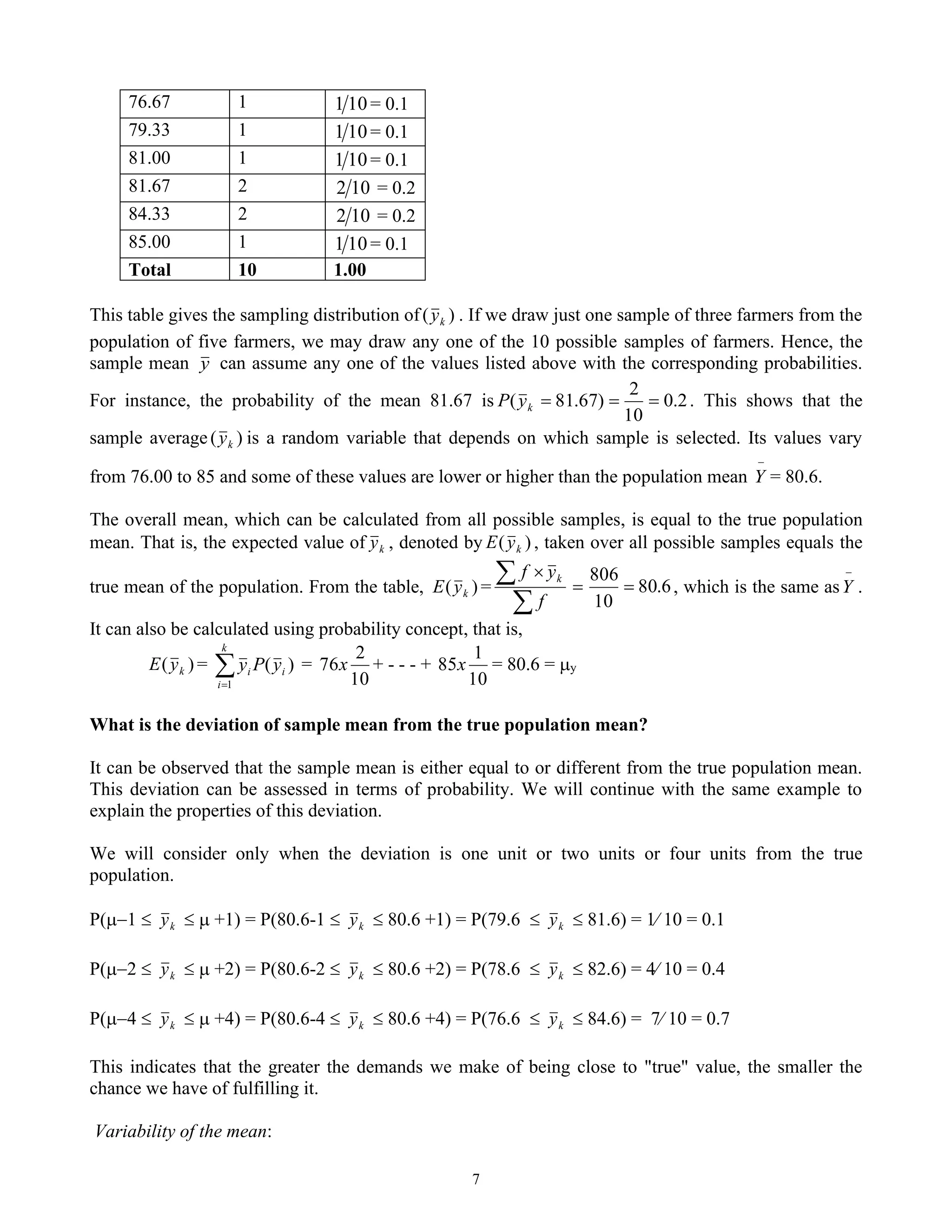
76.00 2 10
2 = 0.2
7
76.67 1 10
1 = 0.1
79.33 1 10
1 = 0.1
81.00 1 10
1 = 0.1
81.67 2 10
2 = 0.2
84.33 2 10
2 = 0.2
85.00 1 10
1 = 0.1
Total 10 1.00
This table gives the sampling distribution of )
( k
y . If we draw just one sample of three farmers from the
population of five farmers, we may draw any one of the 10 possible samples of farmers. Hence, the
sample mean y can assume any one of the values listed above with the corresponding probabilities.
For instance, the probability of the mean 81.67 is 2
.
0
10
2
)
67
.
81
( =
=
=
k
y
P . This shows that the
sample average )
( k
y is a random variable that depends on which sample is selected. Its values vary
from 76.00 to 85 and some of these values are lower or higher than the population mean
−
Y = 80.6.
The overall mean, which can be calculated from all possible samples, is equal to the true population
mean. That is, the expected value of k
y , denoted by )
( k
y
E , taken over all possible samples equals the
true mean of the population. From the table, )
( k
y
E = 6
.
80
10
806
=
=



f
y
f k
, which is the same as
−
Y .
It can also be calculated using probability concept, that is,
)
( k
y
E = )
(
1
i
k
i
i y
P
y

=
=
10
2
76x + - - - +
10
1
85x = 80.6 = y
What is the deviation of sample mean from the true population mean?
It can be observed that the sample mean is either equal to or different from the true population mean.
This deviation can be assessed in terms of probability. We will continue with the same example to
explain the properties of this deviation.
We will consider only when the deviation is one unit or two units or four units from the true
population.
P(−1  k
y   +1) = P(80.6-1  k
y  80.6 +1) = P(79.6  k
y  81.6) = 1 10 = 0.1
P(−2  k
y   +2) = P(80.6-2  k
y  80.6 +2) = P(78.6  k
y  82.6) = 4 10 = 0.4
P(−4  k
y   +4) = P(80.6-4  k
y  80.6 +4) = P(76.6  k
y  84.6) = 7 10 = 0.7
This indicates that the greater the demands we make of being close to "true" value, the smaller the
chance we have of fulfilling it.
Variability of the mean:
8
The Sampling variance of the mean, V( y ), is defined as the average of the squared deviations of the
sample means from the true mean, that is, V
k
k
Y
y
Y
y
E
y i
i
i

=
−
=
−
= 1
2
2
)
(
)
(
)
( , where k is the total
number of possible samples, i
y is the mean of ith
sample and
−
Y is the true mean of the population.
The square root of the sampling variance, )
(y
Var , is called the standard error (S.E.) of the mean of
the sample. The smaller the standard error of the mean, the greater is its reliability.
For each possible ith
sample, we can compute sample variance ( 2
i
s ). Then, the mean of the sample
variance ( 2
s ) is equal to the population variance ( S y
2
), i.e. E
k
s
s
k
i
i

=
=
1
2
2
)
( = S y
2
, where k is total number
of possible samples.
Consider again example 2.1, the population consisting of 5 farmers. The sample variances for all 10
possible samples of size 3 can be computed as:
,
1
)
( 2
1
2
−
−
=

=
n
y
n
y
s
i
j
ij
i where
n
y
y
n
j
ij
i

=
=
1
, for ith
sample with sample size j = 3.
( ) 28
2
56
2
)
76
80
(
)
76
78
(
76
70 2
2
2
2
1 =
=
−
+
−
+
−
=
s ,
( ) 28
2
56
2
)
76
80
(
)
76
78
(
76
70 2
2
2
2
2 =
=
−
+
−
+
−
=
s ,
.
.
.
75
2
150
2
)
85
95
(
)
85
80
(
)
85
80
( 2
2
2
2
10 =
=
−
+
−
+
−
=
s
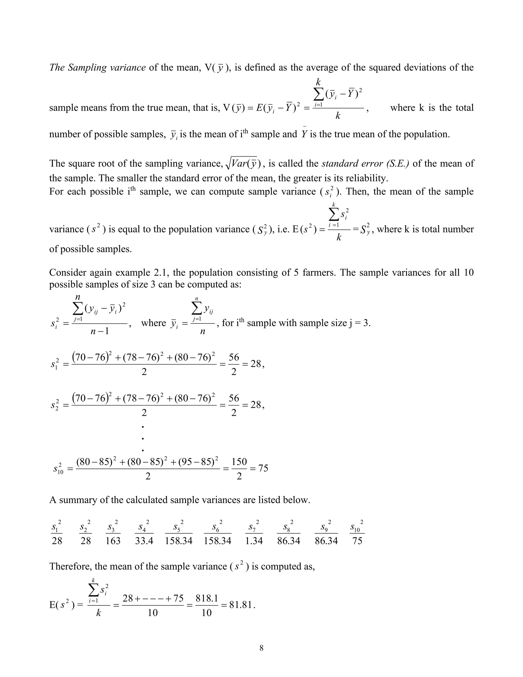
A summary of the calculated sample variances are listed below.
28
2
1
s
28
2
2
s
163
2
3
s
4
.
33
2
4
s
34
.
158
2
5
s
34
.
158
2
6
s
34
.
1
2
7
s
34
.
86
2
8
s
34
.
86
2
9
s
75
2
10
s
Therefore, the mean of the sample variance ( 2
s ) is computed as,
E( 2
s ) = 81
.
81
10
1
.
818
10
75
28
1
2
=
=
+
−
−
−
+
=

=
k
s
k
i
i
.
9
We know that the population variance is S y
2
= 81.8, and this shows that E ( 2
2
) S
s = with some
rounding errors. But the sampling variance, V( y ), is not the same as the population variance ( S
2
), that
is, V( y ) 2
S
 . The equality can be established using the following relationship.
V( y ) = ( ),
1
2
f
n
S
− where (1-f) is a finite population correction (fpc).
This shows that sampling variance, V( y ), depends on the population parameter S
2
, which is mostly
known, but should be estimated by sample variance.
EX. Verify that V( y ) 2
S

2.4 Properties of Estimates
An estimator is a rule that tells how to calculate an estimate based on the measurements contained in a
sample. It is a sample statistic used to estimate a population parameter. Thus, the sample mean y is an
estimator of the population mean
−
Y . The value (s) assigned to a population parameter based on the
value of a sample statistic is called an estimate. For instance from the above example, 00
.
76
=
k
y is
an estimate of
−
Y .
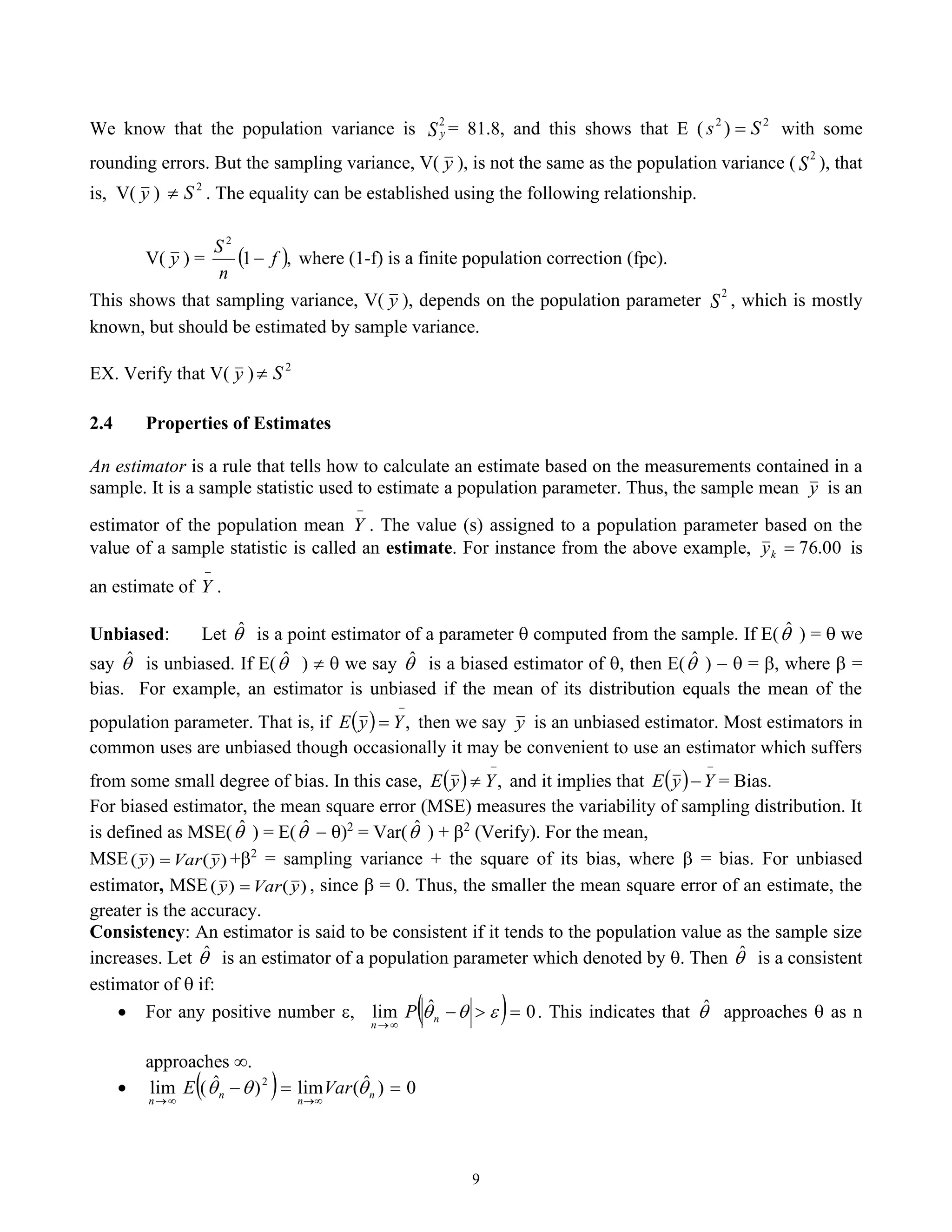
Unbiased: Let 
ˆ is a point estimator of a parameter  computed from the sample. If E(
ˆ ) =  we
say 
ˆ is unbiased. If E(
ˆ )   we say 
ˆ is a biased estimator of , then E(
ˆ ) −  = , where  =
bias. For example, an estimator is unbiased if the mean of its distribution equals the mean of the
population parameter. That is, if ( )
−
= ,
Y
y
E then we say y is an unbiased estimator. Most estimators in
common uses are unbiased though occasionally it may be convenient to use an estimator which suffers
from some small degree of bias. In this case, ( )
−
 ,
Y
y
E and it implies that ( )
−
−Y
y
E = Bias.
For biased estimator, the mean square error (MSE) measures the variability of sampling distribution. It
is defined as MSE(
ˆ ) = E(
ˆ − )2
= Var(
ˆ ) + 2
(Verify). For the mean,
MSE )
(
)
( y
Var
y = +2
= sampling variance + the square of its bias, where  = bias. For unbiased
estimator, MSE )
(
)
( y
Var
y = , since  = 0. Thus, the smaller the mean square error of an estimate, the
greater is the accuracy.
Consistency: An estimator is said to be consistent if it tends to the population value as the sample size
increases. Let 
ˆ is an estimator of a population parameter which denoted by . Then 
ˆ is a consistent
estimator of  if:
• For any positive number , ( ) 0
ˆ
lim =

−

→


n
n
P . This indicates that 
ˆ approaches  as n
approaches .
• ( ) 0
)
ˆ
(
lim
)
ˆ
(
lim 2
=
=
−

→

→
n
n
n
n
Var
E 


10
Example:
An estimator is said to be consistent if it tends to the population value with increasing sample size. As
the size of the sample increases, the sample estimates concentrate around the population value. By
considering the population of 5 farmers, we can find all possible samples of size 2, 3, and 4 without
replacement and compute the sample results. The sampling distribution is has already been calculated
when the sample size is three and in similar way the sampling distributions can be calculated for
sample sizes two and four. The following possible sample means can be observed from three different
sample sizes.
5
.
87
00
.
74 
 y , when the sample size n = 2 with 10 possible samples.
00
.
76 00
.
85

 y , when the sample size n = 3 with 10 possible samples.
25
.
83
00
.
77 
 y , when the sample size n = 4 with 5 possible samples.
This example shows that as the sample size increases, the sample mean tends to the population mean in
both directions.
Efficiency: A particular sampling scheme is said to be more" efficient" than another if, for a fixed
sample size, the sampling variance of survey estimates for the first scheme is less than that for the
second. For the same population often comparisons of efficiency are made with simple random
sampling as a basic scheme using the ratio of their variances.
For example, if 1
y and 2
y are two estimators of a parameterY , with equal sample size, and having
variances, V( 1
y ) and V( 2
y ) respectively, then the efficiency of 1
y relative to 2
y is given as follows.
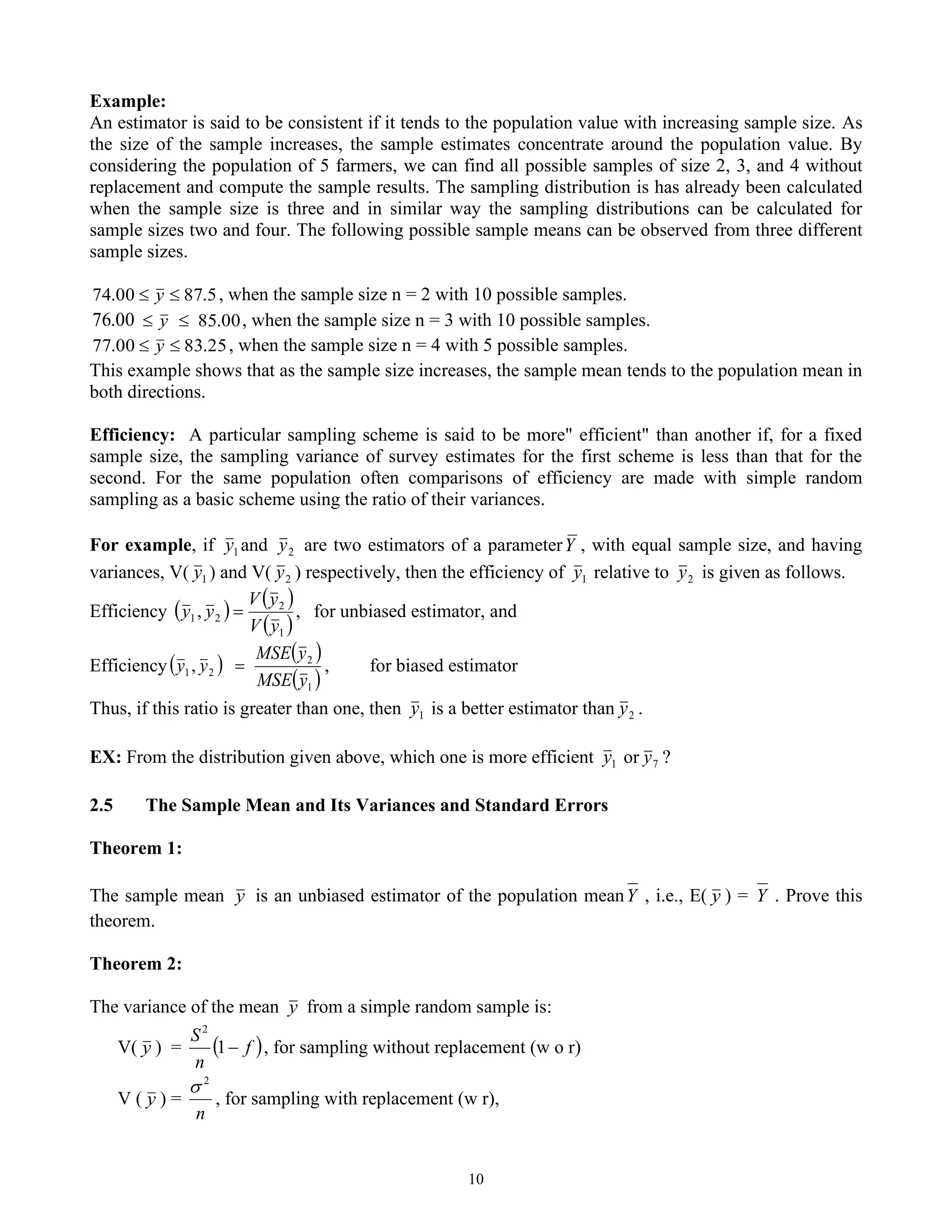
Efficiency ( ) ( )
( )
,
,
1
2
2
1
y
V
y
V
y
y = for unbiased estimator, and
Efficiency( )
( )
( )
1
2
2
1,
y
MSE
y
MSE
y
y = , for biased estimator
Thus, if this ratio is greater than one, then 1
y is a better estimator than 2
y .
EX: From the distribution given above, which one is more efficient 1
y or 7
y ?
2.5 The Sample Mean and Its Variances and Standard Errors
Theorem 1:
The sample mean y is an unbiased estimator of the population meanY , i.e., E( y ) = Y . Prove this
theorem.
Theorem 2:
The variance of the mean y from a simple random sample is:
V( y ) = ( )
f
n
S
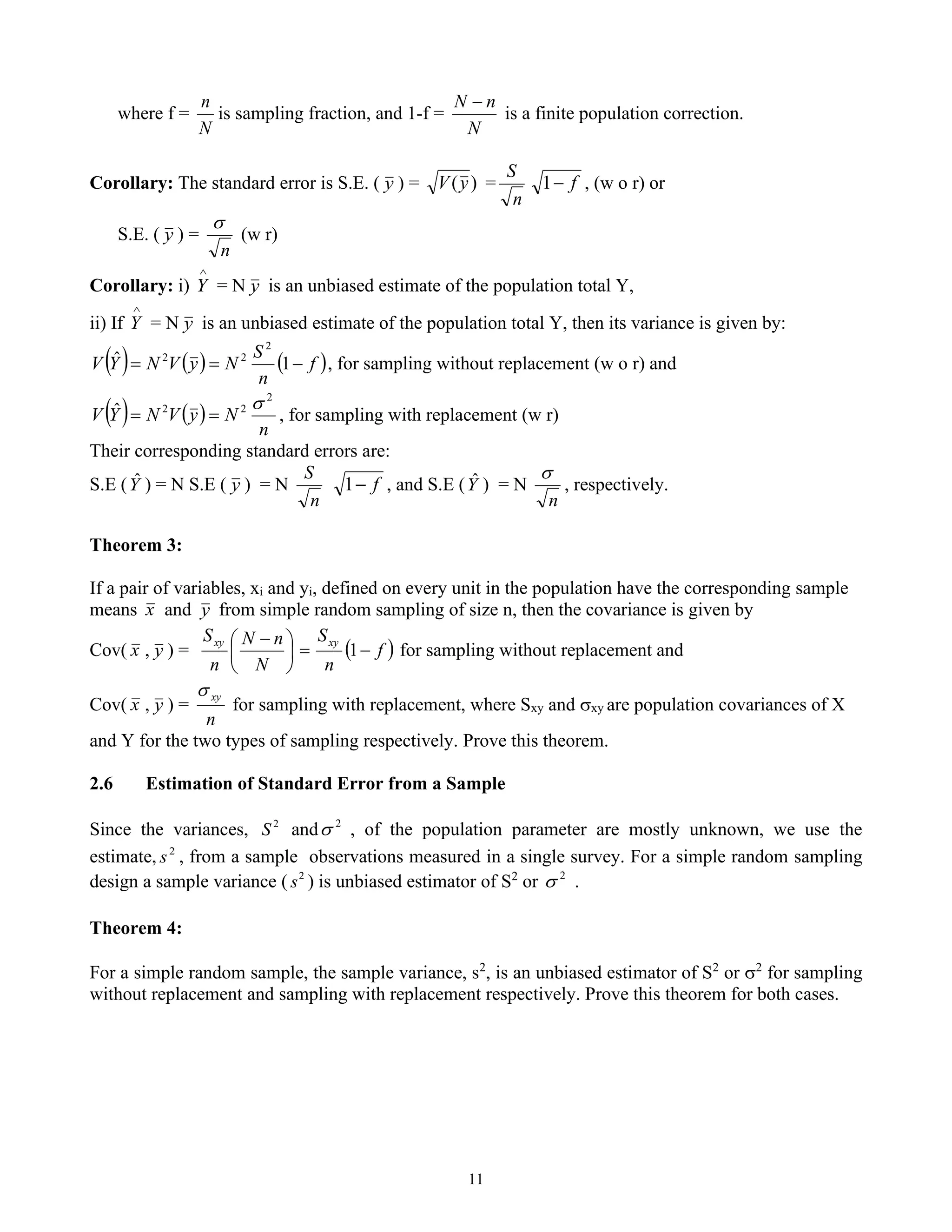
−
1
2
, for sampling without replacement (w o r)
V ( y ) =
n
2

, for sampling with replacement (w r),
11
where f =
N
n
is sampling fraction, and 1-f =
N
n
N −
is a finite population correction.
Corollary: The standard error is S.E. ( y ) = )
(y
V =
n
S
f
−
1 , (w o r) or
S.E. ( y ) =
n

(w r)
Corollary: i)

Y = N y is an unbiased estimate of the population total Y,
ii) If

Y = N y is an unbiased estimate of the population total Y, then its variance is given by:
( ) ( ) ( )
f
n
S
N
y
V
N
Y
V −
=
= 1
ˆ
2
2
2
, for sampling without replacement (w o r) and
( ) ( )
n
N
y
V
N
Y
V
2
2
2
ˆ 
=
= , for sampling with replacement (w r)
Their corresponding standard errors are:
S.E (Y
ˆ ) = N S.E ( y ) = N
n
S
f
−
1 , and S.E (Y
ˆ ) = N
n

, respectively.
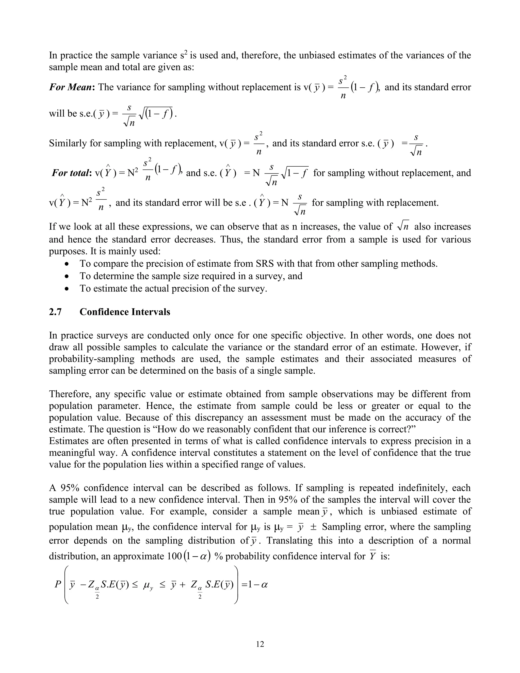
Theorem 3:
If a pair of variables, xi and yi, defined on every unit in the population have the corresponding sample
means x and y from simple random sampling of size n, then the covariance is given by
Cov( x , y ) = ( )
f
n
S
N
n
N
n
S xy
xy
−
=





 −
1 for sampling without replacement and
Cov( x , y ) =
n
xy

for sampling with replacement, where Sxy and xy are population covariances of X
and Y for the two types of sampling respectively. Prove this theorem.
2.6 Estimation of Standard Error from a Sample
Since the variances, 2
S and 2
 , of the population parameter are mostly unknown, we use the
estimate, 2
s , from a sample observations measured in a single survey. For a simple random sampling
design a sample variance ( 2
s ) is unbiased estimator of S2
or 2
 .
Theorem 4:
For a simple random sample, the sample variance, s2
, is an unbiased estimator of S2
or 2
for sampling
without replacement and sampling with replacement respectively. Prove this theorem for both cases.
12
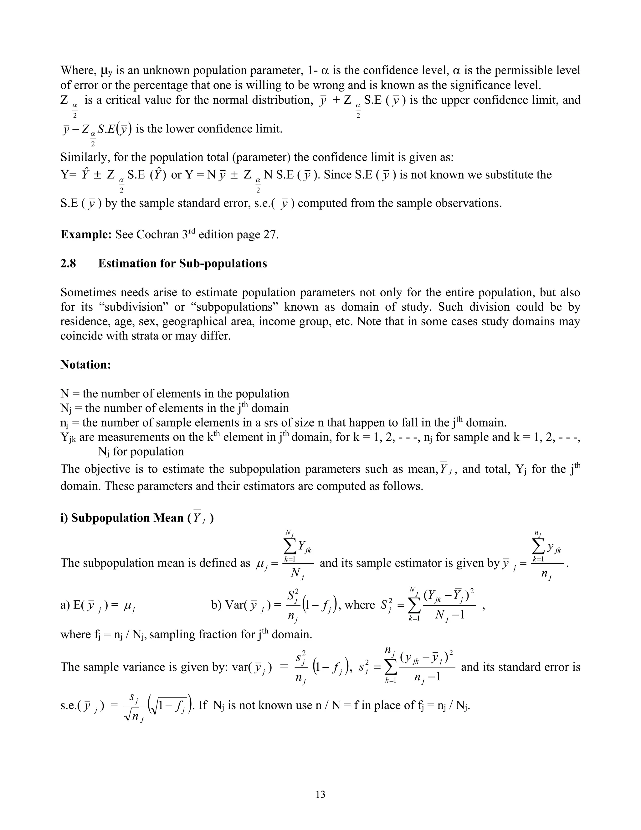
In practice the sample variance s2
is used and, therefore, the unbiased estimates of the variances of the
sample mean and total are given as:
For Mean: The variance for sampling without replacement is v( y ) = ( ),
1
2
f
n
s
− and its standard error
will be s.e.( y ) = ( )
f
n
s
−
1 .
Similarly for sampling with replacement, v( y ) = ,
2
n
s
and its standard error s.e. ( y ) =
n
s
.
For total: v(

Y ) = N2 ( ),
1
2
f
n
s
− and s.e. (

Y ) = N f
n
s
−
1 for sampling without replacement, and
v(

Y ) = N2
n
s2
, and its standard error will be s.e . (

Y ) = N
n
s
for sampling with replacement.
If we look at all these expressions, we can observe that as n increases, the value of n also increases
and hence the standard error decreases. Thus, the standard error from a sample is used for various
purposes. It is mainly used:
• To compare the precision of estimate from SRS with that from other sampling methods.
• To determine the sample size required in a survey, and
• To estimate the actual precision of the survey.
2.7 Confidence Intervals
In practice surveys are conducted only once for one specific objective. In other words, one does not
draw all possible samples to calculate the variance or the standard error of an estimate. However, if
probability-sampling methods are used, the sample estimates and their associated measures of
sampling error can be determined on the basis of a single sample.
Therefore, any specific value or estimate obtained from sample observations may be different from
population parameter. Hence, the estimate from sample could be less or greater or equal to the
population value. Because of this discrepancy an assessment must be made on the accuracy of the
estimate. The question is “How do we reasonably confident that our inference is correct?”
Estimates are often presented in terms of what is called confidence intervals to express precision in a
meaningful way. A confidence interval constitutes a statement on the level of confidence that the true
value for the population lies within a specified range of values.
A 95% confidence interval can be described as follows. If sampling is repeated indefinitely, each
sample will lead to a new confidence interval. Then in 95% of the samples the interval will cover the
true population value. For example, consider a sample mean y , which is unbiased estimate of
population mean μy, the confidence interval for μy is μy = y  Sampling error, where the sampling
error depends on the sampling distribution of y . Translating this into a description of a normal
distribution, an approximate 100 ( )

−
1 % probability confidence interval for Y is:

 
 −
=










+


− 1
)
(
.
)
(
.
2
2
y
E
S
Z
y
y
E
S
Z
y
P y
13
Where, μy is an unknown population parameter, 1-  is the confidence level,  is the permissible level
of error or the percentage that one is willing to be wrong and is known as the significance level.
Z
2
 is a critical value for the normal distribution, y + Z
2
 S.E ( y ) is the upper confidence limit, and
( )
y
E
S
Z
y .
2

− is the lower confidence limit.
Similarly, for the population total (parameter) the confidence limit is given as:
Y= Y
ˆ  Z
2
 S.E )
ˆ
(Y or Y = N y  Z
2
 N S.E ( y ). Since S.E ( y ) is not known we substitute the
S.E ( y ) by the sample standard error, s.e.( y ) computed from the sample observations.
Example: See Cochran 3rd
edition page 27.
2.8 Estimation for Sub-populations
Sometimes needs arise to estimate population parameters not only for the entire population, but also
for its “subdivision” or “subpopulations” known as domain of study. Such division could be by
residence, age, sex, geographical area, income group, etc. Note that in some cases study domains may
coincide with strata or may differ.
Notation:
N = the number of elements in the population
Nj = the number of elements in the jth
domain
nj = the number of sample elements in a srs of size n that happen to fall in the jth
domain.
Yjk are measurements on the kth
element in jth
domain, for k = 1, 2, - - -, nj for sample and k = 1, 2, - - -,
Nj for population
The objective is to estimate the subpopulation parameters such as mean, j
Y , and total, Yj for the jth
domain. These parameters and their estimators are computed as follows.
i) Subpopulation Mean ( j
Y )
The subpopulation mean is defined as
j
N
k
jk
j
N
Y
j

=
= 1
 and its sample estimator is given by
j
n
k
jk
j
n
y
y
j

=
= 1
.
a) E( j
y ) = j
 b) Var( j
y ) = ( )
j
j
j
f
n
S
−
1
2
, where 
= −
−
=
j
N
k j
j
jk
j
N
Y
Y
S
1
2
2
1
)
(
,
where fj = nj / Nj, sampling fraction for jth
domain.
The sample variance is given by: var( j
y ) = ( )
j
j
j
f
n
s
−
1
2
, 
= −
−
=
j
k j
j
jk
j
n
n
y
y
s
1
2
2
1
)
(
and its standard error is
s.e.( j
y ) = ( )
j
j
j
f
n
s
−
1 . If Nj is not known use n / N = f in place of fj = nj / Nj.
14
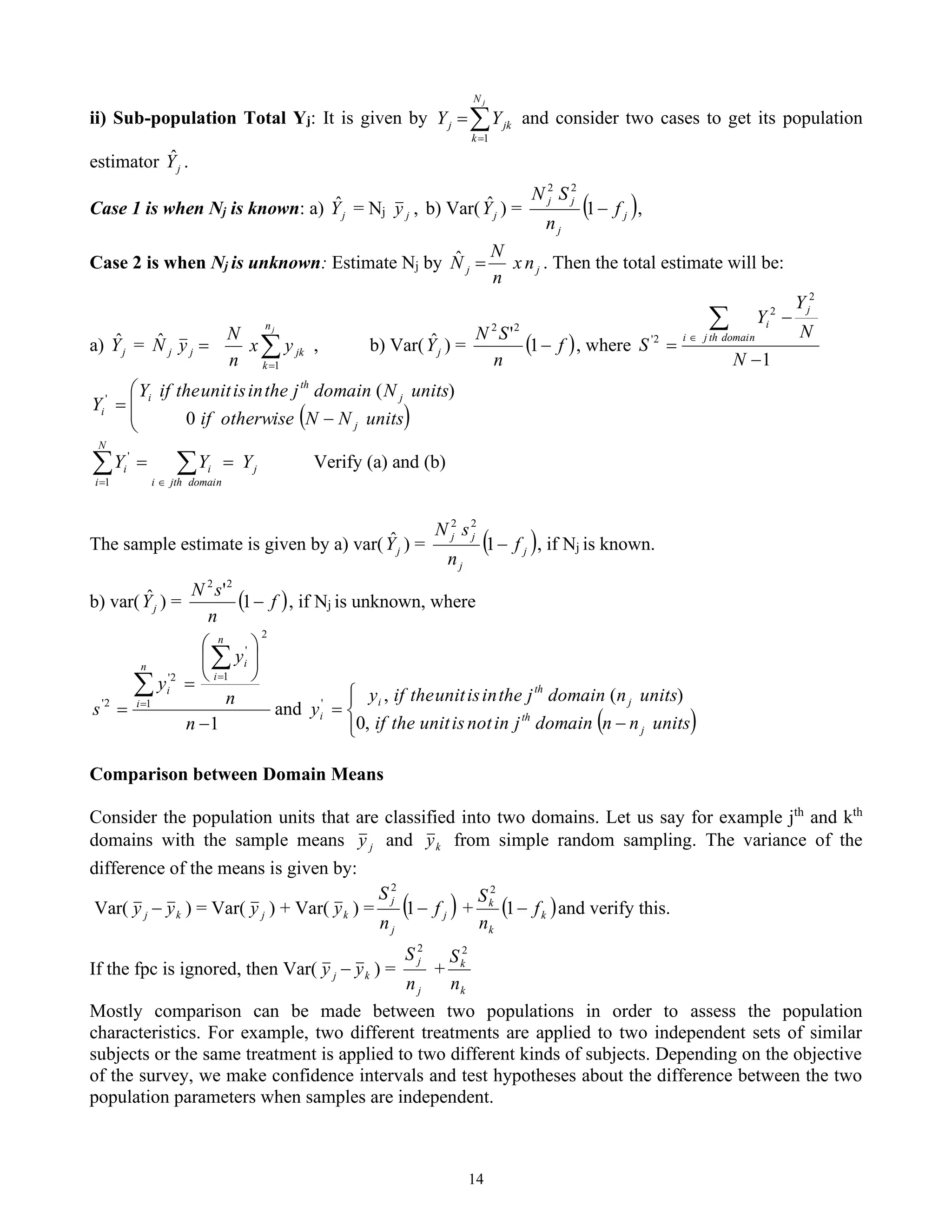
ii) Sub-population Total Yj: It is given by 
=
=
j
N
k
jk
j Y
Y
1
and consider two cases to get its population
estimator j
Ŷ .
Case 1 is when Nj is known: a) j
Ŷ = Nj j
y , b) Var( j
Ŷ ) = ( )
j
j
j
j
f
n
S
N
−
1
2
2
,
Case 2 is when Nj is unknown: Estimate Nj by j
j n
x
n
N
N =
ˆ . Then the total estimate will be:
a) j
Ŷ = =
j
j y
N̂ 
=
j
n
k
jk
y
x
n
N
1
, b) Var( j
Ŷ ) = ( )
f
n
S
N
−
1
'2
2
, where
1
2
2
2
'
−
−
=


N
N
Y
Y
S
domain
th
j
i
j
i
( )




−
=
units
N
N
otherwise
if
units
N
domain
j
the
in
is
unit
the
if
Y
Y
j
j
th
i
i
0
)
(
'

 
=
=
=
domain
jth
i
j
i
N
i
i Y
Y
Y
1
'
Verify (a) and (b)
The sample estimate is given by a) var( j
Ŷ ) = ( )
j
j
j
j
f
n
s
N
−
1
2
2
, if Nj is known.
b) var( j
Ŷ ) = ( )
f
n
s
N
−
1
'2
2
, if Nj is unknown, where
1
1
2
1
'
2
'
2
'
−






=
=


=
=
n
n
y
y
s
n
i
n
i
i
i
and
( )





−
=
units
n
n
domain
j
in
not
is
unit
the
if
units
n
domain
j
the
in
is
unit
the
if
y
y
j
th
j
th
i
i
,
0
)
(
,
'
Comparison between Domain Means
Consider the population units that are classified into two domains. Let us say for example jth
and kth
domains with the sample means j
y and k
y from simple random sampling. The variance of the
difference of the means is given by:
Var( j
y − k
y ) = Var( j
y ) + Var( k
y ) = ( )
j
j
j
f
n
S
−
1
2
+ ( )
k
k
k
f
n
S
−
1
2
and verify this.
If the fpc is ignored, then Var( j
y − k
y ) =
j
j
n
S 2
+
k
k
n
S 2
Mostly comparison can be made between two populations in order to assess the population
characteristics. For example, two different treatments are applied to two independent sets of similar
subjects or the same treatment is applied to two different kinds of subjects. Depending on the objective
of the survey, we make confidence intervals and test hypotheses about the difference between the two
population parameters when samples are independent.
15
2.9 Sample Size Determination for One Item
In the planning of a sample survey one of the first considerations is the sample size determination.
Since every survey is different, there can be no hard and fast rules for determining sample size.
Generally, the factors, which decide the scale of the survey operations, have to do with cost, time,
operational constraints and the desired precision of the results. Once these points have been appraised
and individually assessed, the investigators are in a better position to decide the size of the sample.
2.9.1 Desired Precision of Sample Estimates
One of the major considerations in deciding sample size has to do with the level of error that one
deems tolerable and acceptable. We know that measures of sampling error such as standard error or
coefficient of variation are frequently used to indicate the precision of sample estimates. Since it is
desirable to have high levels of precision, it is also desirable to have large sample sizes, since the larger
the sample, the more precise estimates will be. The sample size can be determined by specifying the
precision required for each major finding to be produced from the survey.
The sample size required under simple random sampling for estimation of population mean y
 is as
follows. Consider that the sample estimate y differs in absolute value from the true unknown mean
y
 by no more than d , i.e., an absolute error Y
y
d −
= or relative error


−
=
y
in which 

=
d .
Specifying maximum allowable difference between y and y
 , and allowing for a small probability 
that the error may exceed that difference, choose a sample size n such that P( y - y
 > d)  .
With SRS we can show that, assuming the estimate y has a standard normal distribution, the sample
n must satisfy the relation given by 2
2
2
2
2
2
1 Nd
S
Z
d
S
Z
n
+
 or
N
n
n
n
o
o
+

1
, where 2
2
2
d
S
Z
no = and Z
is the reliability coefficient which denote the upper 2
 point of standard normal distribution.
If the population size N is very much greater than the required sample size n , the relation above can
be approximated by 2
2
2
d
S
Z
n  or o
n
n  . As a first approximation calculate 2
2
2
d
S
Z
no = . If N
no , the
sampling fraction is very small, say less than 5%, we may consider o
n as a satisfactory approximation
to the required sample size n . Otherwise calculate using the given formula,
N
n
n
n
o
o
+
=
1
.
If we use the relative error Y
d 
= , then we get
2
2
2
2
2






=
=
d
S
Z
d
S
Z
no
( )
2
2
)
(
2
2
2
2


y
CV
Z
Y
S
Z
=
= , where
CV(y) is coefficient of variation.
2.9.2 Sample Size with More Than One Item
In practical situations more variables are used as the basis for calculation of sample size. The decision
on sample size will in fact be largely governed by the way the results are to be analyzed, so that the
investigator must at the outset consider, at least in broad terms, the breakdowns or sub-populations to
16
be made in the final tabulations. Such populations might be defined in terms of age/sex groups or
geographic areas. In the “multi-purpose” nature of most surveys we also deal with many variables in
which an estimation of sample size is needed separately for each variable.
The sample size falling into each sub-population (variable) should be large enough to enable estimates
to be produced at specified levels of precision. Therefore, several of the most important variables are
chosen and sample sizes are calculated for each of these variables. The final sample size chosen might
then be the largest of these calculated sample sizes. If funds are not available to take the largest of
these calculated sample sizes, then, as a compromise measure, the median or mean of the calculated
s
n might be taken.
2.10 Relative Error
Statistical measures such as standard deviation and the standard error appear in the units of
measurement of variables. Such measurement units may cause difficulties in making some
comparisons. Relative measures, such as coefficients of variation, can be used to overcome the
problems.
The element coefficient of variation can be expressed as
Y
S
y
CV
y
=
)
( and estimated by
y
s
y
cv
y
=
)
( .
For the mean ( y ), the coefficient of variation is given by
Y
y
E
S
y
CV
)
.(
.
)
( = , and estimated by
y
y
e
s
y
cv
)
(
)
( = . For the total (Y
ˆ ), the coefficient of variation is given by
)
ˆ
(
)
ˆ
.(
.
)
ˆ
(
Y
E
Y
E
S
Y
CV = , and
estimated by
y
y
e
s
y
N
y
e
s
N
Y
cv
)
(
)
(
)
ˆ
( =
= , which is the same as the coefficient of variation of the mean.
Example: A sample survey of retail outlets is to be conducted in a city that contains 2,500 outlets. The
objective is to estimate the average retail price of 20 items of a commonly used food. An estimate is
needed that is within 10% of the true of the average retail price in the city. An SRS will be taken from
available list of all outlets. Another survey from the same population showed an average price of $
7.00 for 20 items with a standard deviation of $1.4. Assuming 99.7% confidence internal, determine
the sample size.
Solution: 2500
=
N s = 1.4 s2
= (1.4)2
 = 0.1 00
.
7
=
y
( )
( )
( )
%
5
0144
.
0
2500
36
,
36
1
.
0
04
.
0
3
)
(
%,
7
.
99
3
,
04
.
0
7
4
.
1
)
(
0
2
2
2
2
2
0
2
2
2
2
2

=
=
=
=
=
=
=
=
=
N
n
y
CV
Z
n
for
Z
y
s
y
CV

36
0 =
=
 n
n , which is a good approximation for the sample. But if you calculate for n, you will get
that 36
5
.
35
0144
.
0
1
36
2500
36
1
36
1 0
0

=
+
=
+
=
+
=
N
n
n
n
2.11 Limitations of Simple Random Sampling
17
Under simple random sampling any particular sample of n elements from a population of N elements
can be chosen and in addition, is as likely to be chosen as any other sample. In this sense, it is
conceptually the simplest possible method, and hence it is one against which all other methods can be
compared. However, despite such importance, simple random sampling has the following limitations:
• It can be expensive and often not feasible in practice since it requires that all elements be
identified and labeled prior to the sampling. This prior identification is not possible, and hence
a simple random sample of elements cannot be drawn.
• Since it gives each element in the population an equal chance of being chosen in the sample, it
may result in samples that are spread out over a large geographic area. Such a geographic
distribution of the sample would be very costly to implement.
• It would not be good for those surveys in which interest is focused on subgroups that comprise
a small proportion of the population. For example, it is not likely to be an efficient design for
rare events such as disability and special crops.

Short note for sampling theory and research method

  • 1.
    1 Chapter 2: Single-StageSimple Random Sampling After a target population is defined and decision is made to use sample survey as a method of data collection, there are several methods of statistical sampling techniques to use for the intended purpose. These include simple random sampling, stratified random sampling, systematic sampling, cluster sampling and multi-stage sampling. All of these techniques have one sampling characteristic in common. Each deals with a method of random sample selection from a defined target population to be investigated. The random selection procedure ensures that each population unit has an equal chance of being included in the sample. It is this random selection method that provides representative samples impartially and without bias by avoiding any influence of human being. Each technique will be discussed in subsequent chapters. This chapter will present the basic principles and characteristics of single-stage simple random sampling technique. Simple random sampling is very important as a basis for development of the theory of sampling. It serves as a central reference for all other sampling designs. 2.1 Definition and Basic Concepts Simple random sampling (SRS) is a basic probability sampling selection technique in which a predetermined number of sample units are selected from a population list (sampling frame) so that each unit on the list has an equal chance of being included in the sample. Simple random sampling also makes the selection of every possible combination of the desired number of units equally likely. In this way, each sample has an equal chance of being selected. If the population has N units then a random method of selection is one which gives each of the N units in the population to be covered a calculable probability of being selected. To undertake a sample selection, there are two types of random sampling selection−sampling with replacement (wr) and sampling without replacement (w o r). Sampling Without Replacement: Sampling without replacement (wor) means that once a unit has been selected, it cannot be selected again. In other words, it means that no unit can appear more than once in the sample. If there are n sample units required for selection from a population having N units, then there are         n N ways of selecting n units out of a total of N units without replacement, disregarding the order of the n units. Hence, simple random sampling is equivalent to the selection of one of the         n N possible samples with an equal probability         n N 1 assigned to each sample. In simple random sampling without replacement the probability of a specified unit of the population being selected at any given draw is equal to the probability of its being selected at the first draw, that is, N 1 . However, for a sample of size n, the sum of the probabilities of these mutually exclusive events is N n . Sampling with replacement:
  • 2.
    2 The process ofsampling with replacement (wr) allows for a unit to be selected on more than one draw. There are Nn ways of selecting n units out of a total of N units with replacement. In this case, the order of selection will be considered. All selections are independent since the selected unit is returned to the population before making the next selection. Thus, the probability is N 1 for any specific element on each of the n draws. Simple random sampling with or without replacement is practically identical if the sample size is a very small fraction of the population size. Generally, sampling without replacement yields more precise results and is operationally more convenient. 2.2 Simple Random Sample Selection Procedures In sample survey when sample units are selected from a population there could be possibilities of biases in the selection procedure which may come from the use of a non-random method. That is, the selection is consciously or unconsciously influenced by subjective judgment of human being. Such bias can be avoided by using a random selection method. The true randomness can be ensured by using the method of selection which cannot be affected by human influence. There are different random sample selection methods. The important aspect of random selection in each method is that the selection of each unit is based purely on chance. This chance is known as probability of selection which eliminates selection bias. If there is a bias in the selection, it may prevent the sample from being representative of the population. Representative means that probability samples permits scientific approaches in which the samples give accurate estimates of the total population. We consider here two basic and common procedures of random selection method. Lottery Method: This is a very common method of taking a random sample. Under this method, we label each member of the population by identifiable disc or a ticket or pieces of paper. Discs or tickets must be of identical size, color and shape. They are placed in a container (urn/bowl) and well mixed before each draw, and then without looking into the container selection of designated labels will be performed with or without replacement. Then series of drawing may be continued until a sample of the required size is selected. This procedure shows that selection of each item depends entirely on chance. For example, if we want to take a sample of 18 persons out of a population of 90 persons, the procedure is to write the names of all the 90 persons on separate slips (tickets) of paper. The slips (tickets) of paper must be of identical size, color and shape. The next step is to fold these slips, mix them thoroughly and then make a blindfold selection of 18 slips one at a time without replacement. This lottery method becomes quite cumbersome and time consuming to use as the sizes of sample and population increase. To avoid such problems and to reduce the labor of selection process, another method known as a random number table selection process can be used. The Use of Random Numbers: A table of random numbers consists of digits from 0 to 9, which are equally represented with no pattern or order, produced by a computer random number generator. The members of the population are numbered from 1 to N and n numbers are selected from one of the random tables in any convenient and systematic way. The procedure of selection is outlined as follows.
  • 3.
    3 • Identify thepopulation units (N) and give serial numbers from 1 to N. This total number N determines how many of the random digits we need to read when selecting the sample elements. This requires preparation of accurate sampling frame. • Decide the sample size (n) to be selected, which will indicate the total serial numbers to be selected. • Select a starting point of the table of random numbers; you can start from any one of the columns, which can be determined randomly. • Since each digit has an equal chance of being selected at any draw, you may read down columns of digits in the table. • Depending on the population size N, you can use numbers in pairs, three at a time, four at a time, and so on, to read from the table. • If selected numbers are less or equal to the population size N, then they will be considered as sample serial numbers. • All selected numbers greater than N should be ignored. • For sampling without replacement, reject numbers that come up for a second time. • The selection process continues until n distinct units are obtained. For example, consider a population with size N = 5000. Suppose it is desired to take a sample of 25 items out of 5000 without replacement. Since N = 5000, we need four digit numbers. All items from 1 to 5000 should be numbered. We can start anywhere in the table and select numbers four at a time. Thus, using a random table found at the end of this chapter, if we start from column five and read down columns then we will obtain 2913, 2108, 2993, 2425, 1365, 1760, 2104, 1266, 4033, 4147, 0334 4225, 0150, 2940, 1836,1322, 2362, 3942, 3172, 2893, 3933, 2514, 1578, 3649, 0784 by ignoring all numbers greater than 5000. 2.3 Review of Sampling Distribution Basic Notations: We will adapt to use the following basic notations to represent population parameters or sample statistics. These notations will be used throughout this book, but slight modifications will be made to suit the specific design to be considered. For Population parameters: N = the total number of units in the population (population size). i Y = Value of the "y" variable for i th population element (i =1, 2, - - -, N).  = = N i i Y Y 1 is the population total for the "y" Variable N Y N Y Y N i i  = = = 1 = y is the population mean per element of the i Y variable. We will use Y and y interchangeably.
  • 4.
    4 N Y Y N i i y  = − = 1 2 2 ) (  , 1 ) ( 1 2 2 − − =  = N Y Y S N i i yis the variance of population element The relationship between these two variances can be established by expressing each variance in terms of the other, i.e., 2 2 2 2 1 1 y y y S N N or N N S − = − =   . Taking the square root of the variance will give the standard deviation of the population elements, which is represented by y y or S  . Sxy = ( )( ) 1 1 − − −  = N Y Y N X X i i i or σxy = ( )( ) N Y Y N X X i i i − −  =1 is the covariance of the random variable X and Y. y x xy xy S S S =  or y x xy xy     = is the population correlation coefficient For Sample Statistics: n = the number of sample units selected from the population (the sample size) yi = Value of the i y variable for i th sample element (i = 1, 2, - - -, n). y =  = n i i y 1 is the sample total for the “y “variable, n y n y y n i i = =  =1 is the sample mean per element of the " y " variable. s 2 y = 1 ) ( 1 2 − −  = n n y y i i is the variance of the sample elements, and its square root denoted by y s is the standard deviation of the sample elements. sxy = ( )( ) 1 1 − − −  = n y y n x x i i i is sample covariance y x y x s s s = ̂ is sample correlation coefficient f = N n is sampling fraction The sample statistics are computed from the results of sample surveys since the primary objective of a sample survey is to provide estimates of the population parameters, because the reality shows that almost all population parameters are unknown.
  • 5.
    5 Sampling Variability The samplestatistics, calculated from selected sample units, are subject to sampling variability. They depend on the number of sample units (sample size) and types of units included in the sample. Each unit in the population has different characteristic and/or value. For example, a salary of employees varies from individuals to individuals in which the magnitude of salary to be used in the calculation of average income depends on the types of employees selected from the totals workers. Similarly the number of sample workers selected (sample size) will affect the sample values. This indicates that the sample statistics such as mean, total, variance, ratio and proportion are random variables. Like other random variables, these sample statistics possess a probability distribution, which is more commonly known as sampling distribution. Sampling Distribution: What is sampling distribution? What is the purpose of computing sampling distribution? The following example will illustrate the basic idea of sampling distribution and its use. Example 2.1: For demonstration purpose we will consider a very small hypothetical population of 5 farmers, who use fertilizer in their farming. Suppose the amount of fertilizer used (in kg) by each farmer is 70, 78, 80, 80, and 95. Then, the following parameters of the population and sample values (statistics) are computed to justify the basic idea behind estimation. Population Parameters: Let i Y denotes the amount of fertilizer used by each farmer (i =1, 2, - - -, 5). The population size is 5, i.e. N = 5. The total amount of fertilizer used by all farmers and the average fertilizer consumption per farmer are computed as follows. The total amount of fertilizer used is  = = N i i Y Y 1 = 70 + 78 + 80 + 80 + 95 = 403 kg. The mean consumption of fertilizer per farmer is N Y Y = = = 5 403 80.6 kg. Regarding fertilizer consumption variability among farmers, both types of population variances and their corresponding standard deviations are calculated. 1 ) ( 2 2 − − =  N Y Y S i y 2 2 2 2 2 4 ) 6 . 80 95 ( ) 6 . 80 80 ( ) 6 . 80 80 ( ) 6 . 80 78 ( ) 6 . 80 70 ( − + − + − + − + − = 8 . 81 4 2 . 327 2 = = y S . N Y Yi y  − = 2 2 ) (  = 44 . 65 5 2 . 327 = Taking the square root of each variance gives standard deviation of the population, which gives
  • 6.
    6 S y =9.044, and 089 . 8 = Y  . In reality all these population characteristics are mostly unknown for relatively large size of population and should be estimated from survey results collected and summarized from sample elements. Now we want to estimate these population values from sample elements assuming that population parameters are unknown. In the following sampling distribution we will examine all possible samples. Assume that sample of three farmers are selected from the total farmers to estimate the population parameters. The total number of possible samples can be calculated as         n N =         3 5 = 10. The following table shows the ten possible samples with their corresponding values and sample means. Let Fi represents the ith farmer, i = 1, 2, - - - , 5. Types of Sample Units Value for each Sample element Sample Mean ) ( k y 1 3 2 1 F F F 70,78,80 76.00 2 4 2 1 F F F 70,78,80 76.00 3 5 2 1 F F F 70,78,95 81.00 4 4 3 1 F F F 70,80,80 76.67 5 5 3 1 F F F 70,80,95 81.67 6 5 4 1 F F F 70,80,95 81.67 7 4 3 2 F F F 78,80,80 79.33 8 5 3 2 F F F 78,80,95 84.33 9 5 4 2 F F F 78,80,95 84.33 10 5 4 3 F F F 80,80,95 85.00 The Sample Mean: For each possible sample, dividing the sum of the amount of fertilizer used by the size of a sample would give the sample mean ) ( k y . For instance, the mean of the first sample is 3 80 78 70 + + = 76.00, and the remaining sample means can be calculated in a similar way. From the values of random variable k y , we can construct the frequency distribution as shown below. From this frequency we obtain the probabilities of the random variable k y , by dividing the frequency of the random variable k y by the sum of the frequencies. Values of k y Frequency (f) Probability of k y 76.00 2 10 2 = 0.2
  • 7.
    7 76.67 1 10 1= 0.1 79.33 1 10 1 = 0.1 81.00 1 10 1 = 0.1 81.67 2 10 2 = 0.2 84.33 2 10 2 = 0.2 85.00 1 10 1 = 0.1 Total 10 1.00 This table gives the sampling distribution of ) ( k y . If we draw just one sample of three farmers from the population of five farmers, we may draw any one of the 10 possible samples of farmers. Hence, the sample mean y can assume any one of the values listed above with the corresponding probabilities. For instance, the probability of the mean 81.67 is 2 . 0 10 2 ) 67 . 81 ( = = = k y P . This shows that the sample average ) ( k y is a random variable that depends on which sample is selected. Its values vary from 76.00 to 85 and some of these values are lower or higher than the population mean − Y = 80.6. The overall mean, which can be calculated from all possible samples, is equal to the true population mean. That is, the expected value of k y , denoted by ) ( k y E , taken over all possible samples equals the true mean of the population. From the table, ) ( k y E = 6 . 80 10 806 = =    f y f k , which is the same as − Y . It can also be calculated using probability concept, that is, ) ( k y E = ) ( 1 i k i i y P y  = = 10 2 76x + - - - + 10 1 85x = 80.6 = y What is the deviation of sample mean from the true population mean? It can be observed that the sample mean is either equal to or different from the true population mean. This deviation can be assessed in terms of probability. We will continue with the same example to explain the properties of this deviation. We will consider only when the deviation is one unit or two units or four units from the true population. P(−1  k y   +1) = P(80.6-1  k y  80.6 +1) = P(79.6  k y  81.6) = 1 10 = 0.1 P(−2  k y   +2) = P(80.6-2  k y  80.6 +2) = P(78.6  k y  82.6) = 4 10 = 0.4 P(−4  k y   +4) = P(80.6-4  k y  80.6 +4) = P(76.6  k y  84.6) = 7 10 = 0.7 This indicates that the greater the demands we make of being close to "true" value, the smaller the chance we have of fulfilling it. Variability of the mean:
  • 8.
    8 The Sampling varianceof the mean, V( y ), is defined as the average of the squared deviations of the sample means from the true mean, that is, V k k Y y Y y E y i i i  = − = − = 1 2 2 ) ( ) ( ) ( , where k is the total number of possible samples, i y is the mean of ith sample and − Y is the true mean of the population. The square root of the sampling variance, ) (y Var , is called the standard error (S.E.) of the mean of the sample. The smaller the standard error of the mean, the greater is its reliability. For each possible ith sample, we can compute sample variance ( 2 i s ). Then, the mean of the sample variance ( 2 s ) is equal to the population variance ( S y 2 ), i.e. E k s s k i i  = = 1 2 2 ) ( = S y 2 , where k is total number of possible samples. Consider again example 2.1, the population consisting of 5 farmers. The sample variances for all 10 possible samples of size 3 can be computed as: , 1 ) ( 2 1 2 − − =  = n y n y s i j ij i where n y y n j ij i  = = 1 , for ith sample with sample size j = 3. ( ) 28 2 56 2 ) 76 80 ( ) 76 78 ( 76 70 2 2 2 2 1 = = − + − + − = s , ( ) 28 2 56 2 ) 76 80 ( ) 76 78 ( 76 70 2 2 2 2 2 = = − + − + − = s , . . . 75 2 150 2 ) 85 95 ( ) 85 80 ( ) 85 80 ( 2 2 2 2 10 = = − + − + − = s A summary of the calculated sample variances are listed below. 28 2 1 s 28 2 2 s 163 2 3 s 4 . 33 2 4 s 34 . 158 2 5 s 34 . 158 2 6 s 34 . 1 2 7 s 34 . 86 2 8 s 34 . 86 2 9 s 75 2 10 s Therefore, the mean of the sample variance ( 2 s ) is computed as, E( 2 s ) = 81 . 81 10 1 . 818 10 75 28 1 2 = = + − − − + =  = k s k i i .
  • 9.
    9 We know thatthe population variance is S y 2 = 81.8, and this shows that E ( 2 2 ) S s = with some rounding errors. But the sampling variance, V( y ), is not the same as the population variance ( S 2 ), that is, V( y ) 2 S  . The equality can be established using the following relationship. V( y ) = ( ), 1 2 f n S − where (1-f) is a finite population correction (fpc). This shows that sampling variance, V( y ), depends on the population parameter S 2 , which is mostly known, but should be estimated by sample variance. EX. Verify that V( y ) 2 S  2.4 Properties of Estimates An estimator is a rule that tells how to calculate an estimate based on the measurements contained in a sample. It is a sample statistic used to estimate a population parameter. Thus, the sample mean y is an estimator of the population mean − Y . The value (s) assigned to a population parameter based on the value of a sample statistic is called an estimate. For instance from the above example, 00 . 76 = k y is an estimate of − Y . Unbiased: Let  ˆ is a point estimator of a parameter  computed from the sample. If E( ˆ ) =  we say  ˆ is unbiased. If E( ˆ )   we say  ˆ is a biased estimator of , then E( ˆ ) −  = , where  = bias. For example, an estimator is unbiased if the mean of its distribution equals the mean of the population parameter. That is, if ( ) − = , Y y E then we say y is an unbiased estimator. Most estimators in common uses are unbiased though occasionally it may be convenient to use an estimator which suffers from some small degree of bias. In this case, ( ) −  , Y y E and it implies that ( ) − −Y y E = Bias. For biased estimator, the mean square error (MSE) measures the variability of sampling distribution. It is defined as MSE( ˆ ) = E( ˆ − )2 = Var( ˆ ) + 2 (Verify). For the mean, MSE ) ( ) ( y Var y = +2 = sampling variance + the square of its bias, where  = bias. For unbiased estimator, MSE ) ( ) ( y Var y = , since  = 0. Thus, the smaller the mean square error of an estimate, the greater is the accuracy. Consistency: An estimator is said to be consistent if it tends to the population value as the sample size increases. Let  ˆ is an estimator of a population parameter which denoted by . Then  ˆ is a consistent estimator of  if: • For any positive number , ( ) 0 ˆ lim =  −  →   n n P . This indicates that  ˆ approaches  as n approaches . • ( ) 0 ) ˆ ( lim ) ˆ ( lim 2 = = −  →  → n n n n Var E   
  • 10.
    10 Example: An estimator issaid to be consistent if it tends to the population value with increasing sample size. As the size of the sample increases, the sample estimates concentrate around the population value. By considering the population of 5 farmers, we can find all possible samples of size 2, 3, and 4 without replacement and compute the sample results. The sampling distribution is has already been calculated when the sample size is three and in similar way the sampling distributions can be calculated for sample sizes two and four. The following possible sample means can be observed from three different sample sizes. 5 . 87 00 . 74   y , when the sample size n = 2 with 10 possible samples. 00 . 76 00 . 85   y , when the sample size n = 3 with 10 possible samples. 25 . 83 00 . 77   y , when the sample size n = 4 with 5 possible samples. This example shows that as the sample size increases, the sample mean tends to the population mean in both directions. Efficiency: A particular sampling scheme is said to be more" efficient" than another if, for a fixed sample size, the sampling variance of survey estimates for the first scheme is less than that for the second. For the same population often comparisons of efficiency are made with simple random sampling as a basic scheme using the ratio of their variances. For example, if 1 y and 2 y are two estimators of a parameterY , with equal sample size, and having variances, V( 1 y ) and V( 2 y ) respectively, then the efficiency of 1 y relative to 2 y is given as follows. Efficiency ( ) ( ) ( ) , , 1 2 2 1 y V y V y y = for unbiased estimator, and Efficiency( ) ( ) ( ) 1 2 2 1, y MSE y MSE y y = , for biased estimator Thus, if this ratio is greater than one, then 1 y is a better estimator than 2 y . EX: From the distribution given above, which one is more efficient 1 y or 7 y ? 2.5 The Sample Mean and Its Variances and Standard Errors Theorem 1: The sample mean y is an unbiased estimator of the population meanY , i.e., E( y ) = Y . Prove this theorem. Theorem 2: The variance of the mean y from a simple random sample is: V( y ) = ( ) f n S − 1 2 , for sampling without replacement (w o r) V ( y ) = n 2  , for sampling with replacement (w r),
  • 11.
    11 where f = N n issampling fraction, and 1-f = N n N − is a finite population correction. Corollary: The standard error is S.E. ( y ) = ) (y V = n S f − 1 , (w o r) or S.E. ( y ) = n  (w r) Corollary: i)  Y = N y is an unbiased estimate of the population total Y, ii) If  Y = N y is an unbiased estimate of the population total Y, then its variance is given by: ( ) ( ) ( ) f n S N y V N Y V − = = 1 ˆ 2 2 2 , for sampling without replacement (w o r) and ( ) ( ) n N y V N Y V 2 2 2 ˆ  = = , for sampling with replacement (w r) Their corresponding standard errors are: S.E (Y ˆ ) = N S.E ( y ) = N n S f − 1 , and S.E (Y ˆ ) = N n  , respectively. Theorem 3: If a pair of variables, xi and yi, defined on every unit in the population have the corresponding sample means x and y from simple random sampling of size n, then the covariance is given by Cov( x , y ) = ( ) f n S N n N n S xy xy − =       − 1 for sampling without replacement and Cov( x , y ) = n xy  for sampling with replacement, where Sxy and xy are population covariances of X and Y for the two types of sampling respectively. Prove this theorem. 2.6 Estimation of Standard Error from a Sample Since the variances, 2 S and 2  , of the population parameter are mostly unknown, we use the estimate, 2 s , from a sample observations measured in a single survey. For a simple random sampling design a sample variance ( 2 s ) is unbiased estimator of S2 or 2  . Theorem 4: For a simple random sample, the sample variance, s2 , is an unbiased estimator of S2 or 2 for sampling without replacement and sampling with replacement respectively. Prove this theorem for both cases.
  • 12.
    12 In practice thesample variance s2 is used and, therefore, the unbiased estimates of the variances of the sample mean and total are given as: For Mean: The variance for sampling without replacement is v( y ) = ( ), 1 2 f n s − and its standard error will be s.e.( y ) = ( ) f n s − 1 . Similarly for sampling with replacement, v( y ) = , 2 n s and its standard error s.e. ( y ) = n s . For total: v(  Y ) = N2 ( ), 1 2 f n s − and s.e. (  Y ) = N f n s − 1 for sampling without replacement, and v(  Y ) = N2 n s2 , and its standard error will be s.e . (  Y ) = N n s for sampling with replacement. If we look at all these expressions, we can observe that as n increases, the value of n also increases and hence the standard error decreases. Thus, the standard error from a sample is used for various purposes. It is mainly used: • To compare the precision of estimate from SRS with that from other sampling methods. • To determine the sample size required in a survey, and • To estimate the actual precision of the survey. 2.7 Confidence Intervals In practice surveys are conducted only once for one specific objective. In other words, one does not draw all possible samples to calculate the variance or the standard error of an estimate. However, if probability-sampling methods are used, the sample estimates and their associated measures of sampling error can be determined on the basis of a single sample. Therefore, any specific value or estimate obtained from sample observations may be different from population parameter. Hence, the estimate from sample could be less or greater or equal to the population value. Because of this discrepancy an assessment must be made on the accuracy of the estimate. The question is “How do we reasonably confident that our inference is correct?” Estimates are often presented in terms of what is called confidence intervals to express precision in a meaningful way. A confidence interval constitutes a statement on the level of confidence that the true value for the population lies within a specified range of values. A 95% confidence interval can be described as follows. If sampling is repeated indefinitely, each sample will lead to a new confidence interval. Then in 95% of the samples the interval will cover the true population value. For example, consider a sample mean y , which is unbiased estimate of population mean μy, the confidence interval for μy is μy = y  Sampling error, where the sampling error depends on the sampling distribution of y . Translating this into a description of a normal distribution, an approximate 100 ( )  − 1 % probability confidence interval for Y is:     − =           +   − 1 ) ( . ) ( . 2 2 y E S Z y y E S Z y P y
  • 13.
    13 Where, μy isan unknown population parameter, 1-  is the confidence level,  is the permissible level of error or the percentage that one is willing to be wrong and is known as the significance level. Z 2  is a critical value for the normal distribution, y + Z 2  S.E ( y ) is the upper confidence limit, and ( ) y E S Z y . 2  − is the lower confidence limit. Similarly, for the population total (parameter) the confidence limit is given as: Y= Y ˆ  Z 2  S.E ) ˆ (Y or Y = N y  Z 2  N S.E ( y ). Since S.E ( y ) is not known we substitute the S.E ( y ) by the sample standard error, s.e.( y ) computed from the sample observations. Example: See Cochran 3rd edition page 27. 2.8 Estimation for Sub-populations Sometimes needs arise to estimate population parameters not only for the entire population, but also for its “subdivision” or “subpopulations” known as domain of study. Such division could be by residence, age, sex, geographical area, income group, etc. Note that in some cases study domains may coincide with strata or may differ. Notation: N = the number of elements in the population Nj = the number of elements in the jth domain nj = the number of sample elements in a srs of size n that happen to fall in the jth domain. Yjk are measurements on the kth element in jth domain, for k = 1, 2, - - -, nj for sample and k = 1, 2, - - -, Nj for population The objective is to estimate the subpopulation parameters such as mean, j Y , and total, Yj for the jth domain. These parameters and their estimators are computed as follows. i) Subpopulation Mean ( j Y ) The subpopulation mean is defined as j N k jk j N Y j  = = 1  and its sample estimator is given by j n k jk j n y y j  = = 1 . a) E( j y ) = j  b) Var( j y ) = ( ) j j j f n S − 1 2 , where  = − − = j N k j j jk j N Y Y S 1 2 2 1 ) ( , where fj = nj / Nj, sampling fraction for jth domain. The sample variance is given by: var( j y ) = ( ) j j j f n s − 1 2 ,  = − − = j k j j jk j n n y y s 1 2 2 1 ) ( and its standard error is s.e.( j y ) = ( ) j j j f n s − 1 . If Nj is not known use n / N = f in place of fj = nj / Nj.
  • 14.
    14 ii) Sub-population TotalYj: It is given by  = = j N k jk j Y Y 1 and consider two cases to get its population estimator j Ŷ . Case 1 is when Nj is known: a) j Ŷ = Nj j y , b) Var( j Ŷ ) = ( ) j j j j f n S N − 1 2 2 , Case 2 is when Nj is unknown: Estimate Nj by j j n x n N N = ˆ . Then the total estimate will be: a) j Ŷ = = j j y N̂  = j n k jk y x n N 1 , b) Var( j Ŷ ) = ( ) f n S N − 1 '2 2 , where 1 2 2 2 ' − − =   N N Y Y S domain th j i j i ( )     − = units N N otherwise if units N domain j the in is unit the if Y Y j j th i i 0 ) ( '    = = = domain jth i j i N i i Y Y Y 1 ' Verify (a) and (b) The sample estimate is given by a) var( j Ŷ ) = ( ) j j j j f n s N − 1 2 2 , if Nj is known. b) var( j Ŷ ) = ( ) f n s N − 1 '2 2 , if Nj is unknown, where 1 1 2 1 ' 2 ' 2 ' −       = =   = = n n y y s n i n i i i and ( )      − = units n n domain j in not is unit the if units n domain j the in is unit the if y y j th j th i i , 0 ) ( , ' Comparison between Domain Means Consider the population units that are classified into two domains. Let us say for example jth and kth domains with the sample means j y and k y from simple random sampling. The variance of the difference of the means is given by: Var( j y − k y ) = Var( j y ) + Var( k y ) = ( ) j j j f n S − 1 2 + ( ) k k k f n S − 1 2 and verify this. If the fpc is ignored, then Var( j y − k y ) = j j n S 2 + k k n S 2 Mostly comparison can be made between two populations in order to assess the population characteristics. For example, two different treatments are applied to two independent sets of similar subjects or the same treatment is applied to two different kinds of subjects. Depending on the objective of the survey, we make confidence intervals and test hypotheses about the difference between the two population parameters when samples are independent.
  • 15.
    15 2.9 Sample SizeDetermination for One Item In the planning of a sample survey one of the first considerations is the sample size determination. Since every survey is different, there can be no hard and fast rules for determining sample size. Generally, the factors, which decide the scale of the survey operations, have to do with cost, time, operational constraints and the desired precision of the results. Once these points have been appraised and individually assessed, the investigators are in a better position to decide the size of the sample. 2.9.1 Desired Precision of Sample Estimates One of the major considerations in deciding sample size has to do with the level of error that one deems tolerable and acceptable. We know that measures of sampling error such as standard error or coefficient of variation are frequently used to indicate the precision of sample estimates. Since it is desirable to have high levels of precision, it is also desirable to have large sample sizes, since the larger the sample, the more precise estimates will be. The sample size can be determined by specifying the precision required for each major finding to be produced from the survey. The sample size required under simple random sampling for estimation of population mean y  is as follows. Consider that the sample estimate y differs in absolute value from the true unknown mean y  by no more than d , i.e., an absolute error Y y d − = or relative error   − = y in which   = d . Specifying maximum allowable difference between y and y  , and allowing for a small probability  that the error may exceed that difference, choose a sample size n such that P( y - y  > d)  . With SRS we can show that, assuming the estimate y has a standard normal distribution, the sample n must satisfy the relation given by 2 2 2 2 2 2 1 Nd S Z d S Z n +  or N n n n o o +  1 , where 2 2 2 d S Z no = and Z is the reliability coefficient which denote the upper 2  point of standard normal distribution. If the population size N is very much greater than the required sample size n , the relation above can be approximated by 2 2 2 d S Z n  or o n n  . As a first approximation calculate 2 2 2 d S Z no = . If N no , the sampling fraction is very small, say less than 5%, we may consider o n as a satisfactory approximation to the required sample size n . Otherwise calculate using the given formula, N n n n o o + = 1 . If we use the relative error Y d  = , then we get 2 2 2 2 2       = = d S Z d S Z no ( ) 2 2 ) ( 2 2 2 2   y CV Z Y S Z = = , where CV(y) is coefficient of variation. 2.9.2 Sample Size with More Than One Item In practical situations more variables are used as the basis for calculation of sample size. The decision on sample size will in fact be largely governed by the way the results are to be analyzed, so that the investigator must at the outset consider, at least in broad terms, the breakdowns or sub-populations to
  • 16.
    16 be made inthe final tabulations. Such populations might be defined in terms of age/sex groups or geographic areas. In the “multi-purpose” nature of most surveys we also deal with many variables in which an estimation of sample size is needed separately for each variable. The sample size falling into each sub-population (variable) should be large enough to enable estimates to be produced at specified levels of precision. Therefore, several of the most important variables are chosen and sample sizes are calculated for each of these variables. The final sample size chosen might then be the largest of these calculated sample sizes. If funds are not available to take the largest of these calculated sample sizes, then, as a compromise measure, the median or mean of the calculated s n might be taken. 2.10 Relative Error Statistical measures such as standard deviation and the standard error appear in the units of measurement of variables. Such measurement units may cause difficulties in making some comparisons. Relative measures, such as coefficients of variation, can be used to overcome the problems. The element coefficient of variation can be expressed as Y S y CV y = ) ( and estimated by y s y cv y = ) ( . For the mean ( y ), the coefficient of variation is given by Y y E S y CV ) .( . ) ( = , and estimated by y y e s y cv ) ( ) ( = . For the total (Y ˆ ), the coefficient of variation is given by ) ˆ ( ) ˆ .( . ) ˆ ( Y E Y E S Y CV = , and estimated by y y e s y N y e s N Y cv ) ( ) ( ) ˆ ( = = , which is the same as the coefficient of variation of the mean. Example: A sample survey of retail outlets is to be conducted in a city that contains 2,500 outlets. The objective is to estimate the average retail price of 20 items of a commonly used food. An estimate is needed that is within 10% of the true of the average retail price in the city. An SRS will be taken from available list of all outlets. Another survey from the same population showed an average price of $ 7.00 for 20 items with a standard deviation of $1.4. Assuming 99.7% confidence internal, determine the sample size. Solution: 2500 = N s = 1.4 s2 = (1.4)2  = 0.1 00 . 7 = y ( ) ( ) ( ) % 5 0144 . 0 2500 36 , 36 1 . 0 04 . 0 3 ) ( %, 7 . 99 3 , 04 . 0 7 4 . 1 ) ( 0 2 2 2 2 2 0 2 2 2 2 2  = = = = = = = = = N n y CV Z n for Z y s y CV  36 0 = =  n n , which is a good approximation for the sample. But if you calculate for n, you will get that 36 5 . 35 0144 . 0 1 36 2500 36 1 36 1 0 0  = + = + = + = N n n n 2.11 Limitations of Simple Random Sampling
  • 17.
    17 Under simple randomsampling any particular sample of n elements from a population of N elements can be chosen and in addition, is as likely to be chosen as any other sample. In this sense, it is conceptually the simplest possible method, and hence it is one against which all other methods can be compared. However, despite such importance, simple random sampling has the following limitations: • It can be expensive and often not feasible in practice since it requires that all elements be identified and labeled prior to the sampling. This prior identification is not possible, and hence a simple random sample of elements cannot be drawn. • Since it gives each element in the population an equal chance of being chosen in the sample, it may result in samples that are spread out over a large geographic area. Such a geographic distribution of the sample would be very costly to implement. • It would not be good for those surveys in which interest is focused on subgroups that comprise a small proportion of the population. For example, it is not likely to be an efficient design for rare events such as disability and special crops.