1. Evaluating the Influence of Water Column Structure on Repeatable Estimates of Depth
Gabriell Fraser, Landung Setiawan, Erica Sampaga
University of Washington, School of Oceanography
Acknowledgements
CARIS, USA
Miles Logsdon, Ph.D.
School of Oceanography, University of Washington
Abstract
The accuracy and repeatability of bathymetric
surveys of shallow water estuaries are affected
by freshwater influences on the changing
properties of sound velocity during the
diurnal tidal exchange. Sound Velocity Profiles
(SVP) characterize the vertical structure of the
water column which dramatically varies both in
space and time. A multibeam sonar survey
using the Kongsberg EM302 was conducted in
the inland fjord of Puget Sound in Washington
State, USA aboard the R/V Thomas G.
Thompson on 27 October 2014. All post
processing of the acoustic backscatter were
completed using CARIS HIPs ver. 8.1 in the
Spatial Analysis Lab at the University of
Washington. Both actual and simulated sound
velocity profiles were applied in series of
recalculated base surfaces to investigate the
impact of stratification in the water column on
the production of an accurate and repeatable
depth estimate. The results illustrate that the
thickness of layered structures in the vertical
profile is reflected in variations in estimated
depth.
Fig. 1 Five meter CUBE base surface using the true sound velocity. Shown in
green is the cross section profile used in Fig 3.
Discussion
Three CUBE base surfaces were computed using
different sound velocity profiles (SVP). These
surfaces illustrate the influence of different
estuarine water properties on the role of sound
velocity to alter estimates of depth
(Fig.1). Cross sectional comparisons and
difference images were used to assess the
difference in selected regions of the base
surface (Figures 3 & 4 ). All base surfaces are
similar in depth estimates, though differences
along the cross section can be observed. The
greatest maximum difference of 8.77 meters
was observed along the outer beams (Fig.4).
Since the outer beams traveled the furthest, the
opportunity of water properties to affect the
travel time of sound is the greatest. Therefore
the difference between a well mixed and
freshwater lens environment has the greatest
affect on estimates of depth in the use of outer
beams. These differences suggest that sound
velocity does affect the depth estimates created
via the CUBE algorithm.
Methods
140
145
150
155
160
165
170
175
0 500 1000 1500 2000 2500
Depth(m)
Distance (m)
TrueSVP
MixedSVP
FreshSVP
Fig. 3 Cross sectional comparison of base surface depth estimates created from the application of true, freshwater, and mixed
sound velocity profiles.
True Depth: 154.57 m
Mixed Depth: 155.10 m
Fresh Depth: 154.37 m
True Depth: 170.46 m
Mixed Depth: 168.53 m
Fresh Depth: 170.40 m
True Depth: 138.24 m
Mixed Depth: 134.95 m
Fresh Depth: 138.24 m
Fig. 4 Difference in the depth estimates
between base surfaces created from the
application of true and mixed sound velocity
profiles.
0
20
40
60
80
100
120
140
160
180
1490 1490.5 1491 1491.5 1492 1492.5 1493 1493.5 1494
Depth(m)
Sound Velocity (m/s)
0
20
40
60
80
100
120
140
160
180
1490 1490.5 1491 1491.5 1492 1492.5 1493 1493.5 1494
Depth(m)
Sound Velocity (m/s)
0
20
40
60
80
100
120
140
160
180
1400 1450 1500 1550 1600
Depth(m)
Sound Velocity (m/s)
Fig. 2a True sound velocity profile
of the in situ values collected on
the R/V Thomas G. Thompson
cruise on 28 October 2014.
Fig. 2b Freshwater simulated
sound velocity of a body of water
containing a freshwater lens
between 0-20 meters.
Fig. 2c Mixed simulated sound
velocity profile of well mixed
water with a sound velocity of
1500 meters per second.
During post
processing, a series
of CUBE base
surfaces were
created using
different Sound
Velocity Profiles
(SVP); each designed
to simulate potential
estuarine water
proprieties. Each
base surface was
queried for depth at fixed locations (Fig .1). The
true sound velocity profile was acquired using
the shipboard CTD (Fig. 2a). The freshwater SVP
(Fig. 2b) simulates a freshwater lens to the
depth of 20 meters (m), while the mixed SVP
(Fig 2c) simulates a completely mixed water
column to a depth of 200 m. The CUBE surfaces
were calculated at 5 meter resolution using the
Density and Local option. A cross sectional
comparison from the North West corner to the
South East corner of the study area was created
in order to show differences in depth estimates
due to the application of the three different
SVPs in the CUBE algorithm (Fig. 3).