Downloaded 12 times


![1.2. THE SEQUENCE OF NATURAL NUMBERS 11
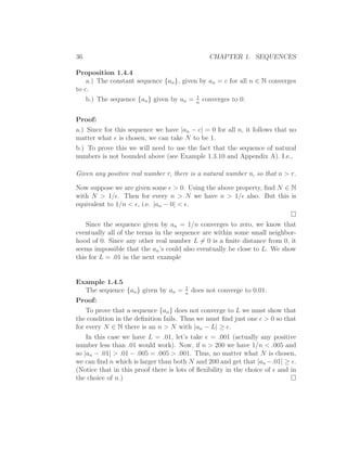
13. a.) Let a and r be positive real numbers and define a geometric sequence
by the recursive formula a1 = a and an = ran−1 , n > 1. Show that
√
an = an+1 an−1 for all n > 1.
b.) Again with a and r positive real numbers define a geometric sequence
√
by the explicit formula an = ar n−1 . Here also, show that an = an+1 an−1
for all n > 1.
14. (Calculator needed.) Find the first 20 terms of the sequences given by
pn+1 = αpn − βp2 where α, β, and p0 are given below. In each case write
n
a sentence or two describing what you think the long term behavior of
the population will be.
a.) α = 2, β = 0.1, p0 = 5.
b.) α = 2.8, β = 0.18, p0 = 5.
c.) α = 3.2, β = 0.22, p0 = 5.
d.) α = 3.8, β = 0.28, p0 = 5.
If you have MAPLE available you can explore this exercise by changing
the values of a and b in the following program:
[> restart:
[> a:=1.2; b:= 0.02;
[> f:=x->a*x - b*x^2;
[> p[0]:=5;
[> for j from 1 to 20 do p[j]:=f(p[j-1]); end do;
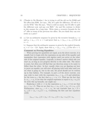
1.2 The sequence of natural numbers
A very familiar and fundamental sequence is that of the natural numbers,
N = {1, 2, 3, ...}. As a sequence, we might describe the natural numbers by
the explicit formula
an = n
but this seems circular. (It certainly does not give a definition of the natural
numbers.) Somewhat more to the point is the recursive description,
an+1 = an + 1, a1 = 1](https://image.slidesharecdn.com/sands807-120904062116-phpapp02/85/Sands807-15-320.jpg)


![1.2. THE SEQUENCE OF NATURAL NUMBERS 17
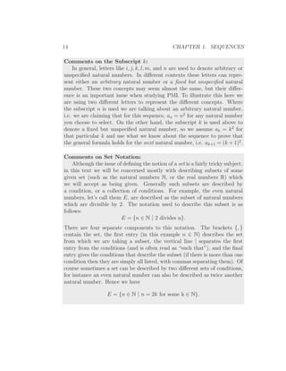
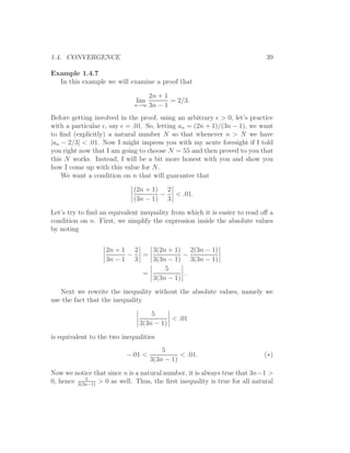
The Principle of Complete Mathematical Induction
Let S be a subset of the natural numbers, N, satisfying
1.) 1 ∈ S
2.) if 1, 2, 3, ..., k are all elements of S, then k + 1 is an element of S as well.
Then S = N.
Example 1.2.5
Let {an } be the sequence given by the two-term recursion formula an+1 =
2an − an−1 + 2 for n > 1 and a1 = 3 and a2 = 6. Listing the first seven
terms of this sequence, we get 3, 6, 11, 18, 27, 38, 51, ... Perhaps a pattern is
becoming evident at this point. It seems that the nth term in the sequence
is given by the explicit formula an = n2 + 2. Let’s use PCMI to prove that
this is the case. Let S be the subset of natural numbers n such that it is true
that an = n2 + 2, i.e.
S = {n ∈ N| an = n2 + 2}.
We know that 1 ∈ S since we are given a1 = 3 and it is easy to check that
3 = 12 + 2. Now assume that we know 1, 2, 3, ..., k are all elements of S. Now,
as long as k > 1 we know that ak+1 = 2ak − ak−1 + 2. Since we are assuming
that k and k − 1 are in S, we can write ak = k 2 + 2 and ak−1 = (k − 1)2 + 2.
Substituting these into the expression for ak+1 we get
ak+1 = 2(k 2 + 2) − [(k − 1)2 + 2] + 2
= 2k 2 + 4 − (k 2 − 2k + 3) + 2
= k 2 + 2k + 3 (1.1)
= (k + 1)2 + 2.
Thus k + 1 ∈ S as well. We aren’t quite done yet! The last argument only
works when k > 1. What about the case that k = 1? If we know that 1 ∈ S
can we conclude that 2 ∈ S? Well, not directly, but we can check that 2 ∈ S
anyway. After all, we are given that a2 = 6 and it is easy to check that
6 = 22 + 2. Notice that if we had given a different value for a2 , then the
entire sequence changes from there on out so the explicit formula would no
longer be correct. However, if you aren’t careful about the subtlety at k = 1,
you might think that you could prove the formula by induction no matter
what is the value of a2 !](https://image.slidesharecdn.com/sands807-120904062116-phpapp02/85/Sands807-21-320.jpg)


![1.4. CONVERGENCE 35
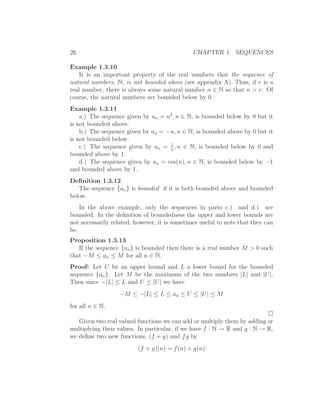
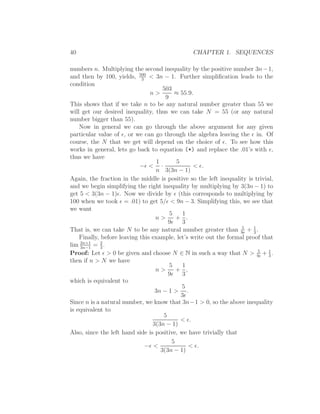
Comments on interval notation:
An interval of real numbers is the set of all real numbers between two
specified real numbers, say a and b. The two specified numbers, a and b, are
called the endpoints of the interval. One, both, or neither of the endpoints
may be contained in the interval. Since intervals are commonly used in
many areas of mathematics, it gets cumbersome to write out the full set
notation each time we refer to an interval, so intervals have been given their
own special shorthand notation. The following equations should be thought
of as defining the notation on the left side of the equality:
(a, b) = {x ∈ R | a < x < b}
[a, b) = {x ∈ R | a ≤ x < b}
(a, b] = {x ∈ R | a < x ≤ b}
[a, b] = {x ∈ R | a ≤ x ≤ b}.
Now, the size of the ǫ-neighborhood around L is determined by ǫ. The
neighborhood gets smaller if the number ǫ gets smaller. Our idea of some
number a giving a good approximation to the number L is that a should be
in some ǫ-neighborhood around L for some small ǫ. Our idea that a sequence
“eventually gives an arbitrarily good approximation” to L should be that no
matter how small we choose ǫ we have that “eventually” all of the elements
of the sequence are in that ǫ-neighborhood. This is made mathematically
precise in the following definition:
Definition 1.4.2
The sequence {an } is said to converge to the real number L if the following
property holds: For every ǫ > 0 there exists an N ∈ N so that |an − L| < ǫ
for every n > N.
If the sequence {an } converges to L, we write
lim an = L.
n→∞
Remark: We will often simply write lim an = L since it is understood that
n → ∞.
Definition 1.4.3
A sequence {an } is said to be convergent if there is some real number L,
so that limn→∞ an = L. If a sequence is not convergent it is called divergent.](https://image.slidesharecdn.com/sands807-120904062116-phpapp02/85/Sands807-39-320.jpg)


![62 CHAPTER 1. SEQUENCES
recursion formula it follows that an+1 > 0, thus a straightforward induction
argument proves that this sequence is bounded below by 0. We also claim
that this sequence is decreasing. To see this we first need to note that a2 =
n
a2
n−1 1 2 a2
n−1 1 an−1 1 2
4
+ a2 + 1, so an − 2 = 4 + a2 − 1 = ( 2 − an−1 ) ≥ 0 for any
n−1 n−1
2
n ≥ 2. Thus we have that an − an+1 = a2 − a1 = a2a−2 ≥ 0 for all n ≥ 1.
n
n
n
n
That is, the sequence is decreasing. Now since we have verified that this
sequence is decreasing and bounded below, we can conclude by the Property
of Completeness that it must converge.
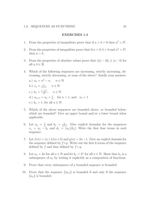
Our first result involves sequences of intervals in R.
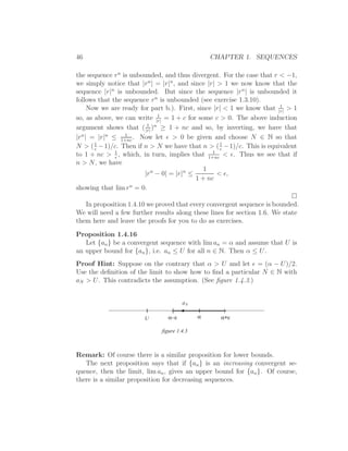
Proposition 1.6.4
Let {An } be a sequence of closed, bounded, intervals in R with the prop-
erty that An+1 ⊂ An for all n ∈ N. Then there is at least one real number α
such that α ∈ An for every n ∈ N.
Since An is a closed interval, we can write it in the interval notation An =
[an , bn ] where an is the left endpoint of the interval, and bn is the right
endpoint. In particular, we have the inequality
an ≤ bn .
Also, since we have An+1 ⊂ An we get the inequalities
an ≤ an+1
and
bn+1 ≤ bn .
Now, the second of these three inequalities tells us that the sequence, {an }, of
left endpoints, is increasing and the third inequality tells us that the sequence,
{bn }, of right endpoints is decreasing. In particular, since {bn } is decreasing
we have that bn ≤ b1 for all n ∈ N, and so, using the first inequality, we
conclude that
an ≤ b1 for all n ∈ N.
Now increasing sequences are always bounded below, so the sequence {an }
is monotone and bounded. Thus we can apply the Property of Completeness
to conclude that the sequence {an } converges to some real number, which
we call α, i.e. lim an = α. To complete the proof we will show that α ∈ An](https://image.slidesharecdn.com/sands807-120904062116-phpapp02/85/Sands807-66-320.jpg)
![1.6. WHAT IS REALITY? 63
for every n ∈ N. This means that we need to show that an ≤ α and α ≤ bn
for every n ∈ N. The first of these inequalities is a direct application of
Proposition 1.4.16 and the second follows from Proposition 1.4.15 and the
observation that for any fixed m ∈ N we have that an ≤ bn ≤ bm for all
n ≥ m and that an ≤ am ≤ bm for all n ≤ m. Thus each bm gives an upper
bound for {an }.
As a corollary to Proposition 1.6.4 we can prove
Proposition 1.6.5
Every bounded sequence in R has a convergent subsequence.
Proof: We begin the proof by using our bounded sequence to define a se-
quence of closed intervals, {An }, with An+1 ⊂ An for each n ∈ N. First, we
start with a sequence {an } which is bounded, i.e., there is some real number
M with the property that |an | < M for all n ∈ N. Let A1 be the closed
interval given by A1 = [−M, M]. Now divide this interval in half to define
the two subintervals B1 and C1 given by B1 = [−M, 0] and C1 = [0, M].
Since all of the points in the sequence are contained in the interval A1 and
also A1 = B1 ∪ C1 , it follows that at least one of the two intervals, B1 or C1
contains infinitely many of the an ’s. Define A2 to be one of these subintervals
which contains infinitely many of the an ’s. Notice that A2 ⊂ A1 . Now do
the same to A2 as we did to A1 . Namely, divide it into two equal closed
subintervals, B2 and C2 . At least one of these two subintervals contains in-
finitely many of the an ’s, so we can choose A3 to be one of these subintervals
which does contain infinitely many of the an ’s. Again, we have A3 ⊂ A2 .
We can continue in this fashion for ever; since we always choose Ai to con-
tain infinitely many of the an ’s we are guarateed that the process does not
stop. Thus we have a sequence of closed intervals satisfying the hypothesis
of Proposition 1.6.3, guaranteeing the result that there is at least one real
number which is contained in all of the An ’s. Choose such a number and call
it α. Also notice that the length of A1 is 2M, the length of A2 is one half of
the length of A1 , i.e. M, etc. In general, the length of An is 22−n M.
The next step of the proof is to describe how we pick an appropriate
subsequence {bn } of {an }. Recall that a subsequence is determined by a
strictly increasing function g : N → N, so to describe {bn } we need only
describe g. To begin with, let g(1) = 1 (so b1 = a1 ). Next, to define g(2),
choose any ak2 in the interval A2 with k2 > 1. Let g(2) = k2 (so b2 = ak2 ).
To define g(3), choose any ak3 ∈ A3 with k3 > g(2) (we know there are](https://image.slidesharecdn.com/sands807-120904062116-phpapp02/85/Sands807-67-320.jpg)


![68 CHAPTER 1. SEQUENCES
c.) Explain why the sequence {an } is bounded above and thus has a
limit, limn→∞ an = α.
d.) Prove that the number α constructed above is a least upper bound
for S by showing that α satisfies properties i.) and ii.) above.
1.7 Some Results from Calculus
Armed with a deeper knowledge of the real numbers, we are now able to
prove some of the most important results about continuous functions on R
that are usually stated without proof in introductory calculus courses. Before
stating the first of these, we need to define continuity on an interval. (The
definition of continuity at a point is given in 1.5.7.)
Definition 1.7.1
A function f : R → R is said to be continuous on the open interval, (a, b),
if it is continuous at every point of (a, b). The function f is continuous on
the closed interval, [a, b] if it is continuous on the open interval (a, b) and
continuous from the right at a and continuous from the left at b.
Of course to make sense of the above, we need the following:
Definition 1.7.2
A function f : R → R is said to be continuous from the right at a if for every
ǫ > 0 there is a δ > 0 so that |f (x) − f (a)| < ǫ whenever 0 ≤ x − a < δ.
(Thus x is within δ of a, but to the right of a.)
Similarly, f is said to be continuous from the left at b if for every ǫ > 0
there is a δ > 0 so that |f (x) − f (b)| < ǫ whenever 0 ≤ b − x < δ.
The first theorem of this chapter is known as the Intermediate Value
Theorem. This theorem is often prosaically interpreted by saying that you
can always draw the graph of a continuous function on a closed interval
without lifting your pencil from the paper. A deeper interpretation is that
this theorem is intimately tied to the fact that there are ”no holes” in the
real number line, i.e. the completeness axiom.](https://image.slidesharecdn.com/sands807-120904062116-phpapp02/85/Sands807-72-320.jpg)
![1.7. SOME RESULTS FROM CALCULUS 69
Theorem 1.7.3
Assume that the function f : R → R is continuous on the closed interval
[a, b], and that f (a) < 0 and f (b) > 0. Then there is some point c ∈ (a, b)
such that f (c) = 0.
Remark: In the exercises we will outline how to generalize this result to
show that, with no restrictions on f (a) and f (b), the function f must attain
every value between the numbers f (a) and f (b).
Proof: The proof is very similar to that of Proposition 1.6.4 in that we will
successively subdivide the interval to define a sequence of numbers, {an }, in
[a, b] which must converge. To do this, begin by naming the interval [a, b] to
be J1 and let a1 = a, and m1 = (b − a)/2, the midpoint of the interval J1 .
There are three cases to consider:
1.) If f (m1 ) = 0 we can stop, by taking c = m1 .
2.) If f (m1 ) > 0 define J2 to be the interval [a, m1 ] and define a2 = a and
b2 = m1 .
3.) Iff (m1 ) < 0 we take J2 to be the interval [m1 , b], and define a2 = m1
and b2 = b.
Notice that J2 = [a2 , b2 ] and f (a2 ) < 0, and f (b2 ) > 0. Thus f satisfies
the conditions of the theorem on J2 . Also notice that b2 − a2 = (b1 − a1 )/2,
i.e. the length of J2 is half of the length of J1 .
Proceeding inductively, suppose that we have found an interval Jk =
[ak , bk ] with f (ak ) < 0, f (bk ) > 0, and the length of Jk equal to 1/2k−1 times
the length of J1 . Let mk = (bk − ak )/2 and consider f (mk ). Again, we
consider three cases:
1.) If f (mk ) = 0, we can stop, and let c = mk .
2.) If f (mk ) > 0 define Jk+1 to be the interval [a, mk ] and define ak+1 = ak
and bk+1 = mk .
3.) Iff (mk ) < 0 we take Jk+1 to be the interval [mk , b], and define ak+1 =
mk and bk+1 = bk .
By this procedure, we either stop at some step, having already found
a point at which f vanishes, or we continue forever, producing an infinite
sequence of nested intervals, {Jk }, with Jk = [ak , bk ] and f (ak ) < 0, f (bk ) > 0,
and bk+1 − ak+1 = (bk − ak )/2k . It is now straightforward to check that the
sequence of left endpoints, {ak }, is increasing and bounded above, while the
sequence of right endpoints, {bk } is decreasing and bounded below. Thus, by
the completeness axiom, these two sequences have limits. Notice also that](https://image.slidesharecdn.com/sands807-120904062116-phpapp02/85/Sands807-73-320.jpg)
![70 CHAPTER 1. SEQUENCES
lim(bk − ak ) = 0, so the two sequences limit to the same point. Call the limit
point c. It remains to show that f (c) = 0. Since f is continuous, we know
that
f (c) = f (lim ak ) = lim f (ak ).
But f (ak ) < 0 for every k, so lim f (ak ) ≤ 0. Likewise
f (c) = f (lim bk ) = lim f (bk ).
And now f (bk ) > 0 for every k, so lim f (bk ) ≥ 0. Having thus shown that
f (c) ≤ 0 and f (c) ≥ 0, we conclude that f (c) = 0.
Our next theorem states that every continuous function f on a closed
interval must be bounded above. (Of course, by applying the theorem to
−f , one can conclude that it is also bounded below as well.)
Theorem 1.7.4
Let f : [a, b] → R be a continuous function on the closed interval [a, b]. Then
there exists an M ∈ R so that f (x) ≤ M for all x ∈ [a, b].
Proof: We proceed by contradiction. Assume to the contrary that no such M
exists. Then for every n ∈ N, there is some point an ∈ [a, b] so that f (an ) > n.
The sequence {an } is bounded, so by Proposition 1.6.5 we conclude that there
must be some subsequence, {bk }, which converges to some number c. Since
the bk ’s are all in [a, b], i.e. a ≤ bk ≤ b it follows that a ≤ c ≤ b, i.e. c ∈ [a, b].
Since f is continuous, we know that f (c) = lim f (bk ), however, it is clear
that lim f (ak ) = ∞ and so lim f (bk ) = ∞ as well. This is a contradiction.
k→∞ k→∞
The final theorem of this section gives the theoretical foundation of the
optimization problems from freshman calculus. In those problems you were
given a function on a closed interval, f : [a, b] → R, and asked to find
c ∈ [a, b] so that f (c) is the maximum value of f on [a, b], i.e. f (c) ≥ f (x)
for all x ∈ [a, b]. This theorem says that such a c must exist.
Theorem 1.7.5
Let f : [a, b] → R be a continuous function on the closed interval [a, b]. Then
there exists c ∈ [a, b] such that f (c) ≥ f (x), for all x ∈ [a, b].
Proof As usual, we will try to construct a sequence that will converge to a
number c that satisfies the required conditions. First, we show that, given](https://image.slidesharecdn.com/sands807-120904062116-phpapp02/85/Sands807-74-320.jpg)
![1.7. SOME RESULTS FROM CALCULUS 71
ǫ > 0, we can find a number c which satisfies the requirements “within ǫ.”
˜
That is, we claim that there is a number c ∈ [a, b] so that f (˜) + ǫ ≥ f (x),
˜ c
for all x ∈ [a, b]. To prove this, consider the sequence bm = f (a) + mǫ for
m = 0, 1, 2, . . . . Now if f (a) ≥ f (x) for all x ∈ [a, b] we can take c = a and be
done with our proof. If this is not the case, then we notice that the sequence
{bm } is increasing and not bounded above. However, since the values of f
are bounded above (by Theorem 1.7.4), there most be some value m0 ∈ N
so that bm0 ≥ f (x) for all x ∈ [a, b] but that bm0 −1 does not satisfy this, i.e.
there is at least one x ∈ [a, b] so that f (x) > bm0 −1 . Choose such an x and
call it c. Then we have f (˜) + ǫ > bm0 −1 + ǫ = bm0 . And since bm0 ≥ f (x)
˜ c
for all x ∈ [a, b], we conclude that f (˜) + ǫ ≥ f (x), for all x ∈ [a, b].
c
Now, for each n ∈ N we can use the above argument to choose a number
1
rn ∈ [a, b] so that f (rn ) + ≥ f (x), for all x ∈ [a, b]. This sequence is
n
bounded, so by Proposition 1.6.5 it must have a convergent subsequence,
let’s call the subsequence {cn } and let the limit of this sequence be called c.
Notice that since the sequence {cn } is a subsequence of {rn } we have that
1 1 1 1
cn + n = rm + n for some m ≥ n, and so cn + n ≥ rm + m ≥ f (x), for all
x ∈ [a, b]. We also have that c ∈ [a, b], since for each n, cn ∈ [a, b].
It remains to show that f (c) ≥ f (x) for all x ∈ [a, b]. Because we assume
that the function f is continuous, we know that the sequence {f (cn )} limits
to f (c). Now let ǫ > 0 be given and chose n ∈ N so that |f (cN ) − f (c)| < ǫ/2
1
and so that N < ǫ/2. Then we have
f (c) − ǫ/2 < f (cN ) < f (c) + ǫ/2.
Adding ǫ/2 to the second inequality, we can conclude that
1
f (c) + ǫ > f (cN ) + ǫ/2 > f (cN ) + ≥ f (x),
N
for all x ∈ [a, b].
Now for each fixed x ∈ [a, b] we have shown that f (c) + ǫ ≥ f (x). Since
ǫ is an arbitrary positive number, we conclude that f (c) ≥ f (x).](https://image.slidesharecdn.com/sands807-120904062116-phpapp02/85/Sands807-75-320.jpg)
![72 CHAPTER 1. SEQUENCES
EXERCISES 1.7
1. Let f (x) be a continuous function on the closed interval [a, b] and let α
be a real number between f (a) and f (b). Show that there is some value,
c ∈ [a, b] such that f (c) = α. (Hint: if f (a) < f (b) apply Theorem 1.7.3
to f (x) − α - make sure you check all of the hypotheses.)
2. Prove that there is a real number x so that sin(x) = x − 1.
3. Use Theorem 1.7.3 to prove that every positive real number, r > 0, has
a square root. (Hint: Consider f (x) = x2 − r on a suitable interval.)
4. Assume that f is a continuous function on [0, 1] and that f (x) ∈ [0, 1]
for each x. Show that there is a c ∈ [0, 1] so that f (c) = c.
5. Suppose that f and g are continuous on [a, b] and that f (a) > g(a)
and g(b) > f (b). Prove that there is some number c ∈ [a, b] so that
f (c) = g(c).
6. a.) Give an example of a continuous function, f, which is defined on the
open interval (0, 1) which is not bounded above.
b.) Give an example of a continuous function, f, which defined on the
open interval (0, 1) and is bounded above, but does not achieve its max-
imum on (0, 1). I.e. there is no number c ∈ (0, 1) satisfying f (c) ≥ f (x)
for all x ∈ (0, 1).
7. a.) Give an example of a function, f, which is defined on the closed
interval [0, 1] but is not bounded above.
b.) Give an example of a function, f , which is defined on the closed
interval [0, 1] and is bounded above, but does not achieve its maximum
on [0, 1].](https://image.slidesharecdn.com/sands807-120904062116-phpapp02/85/Sands807-76-320.jpg)


![2.4. POWER SERIES 99
Corollary 2.4.4
The domain of convergence for a power series an xn is an interval cen-
tered at zero. Thus the domain of convergence has one of the following forms:
[−R, R], (−R, R], [−R, R), (−R, R) with R ≥ 0, or all of R.
Another way of stating this result is that if the power series an xn does
not converge for all real numbers, then there is some nonnegative real number
R so that the power series converges for all real x with |x| < R and diverges
for all real x with |x| > R.
Definition 2.4.5
If R is a nonnegative real number such that the power series an xn
converges for all real x with |x| < R and diverges for all real x with |x| > R
then R is called the radius of convergence for the power series. If the power
series converges for all real numbers, the radius of convergence is said to be
infinite.
Remark: A power series centered at a is a series of the form
an (x − a)n
where a represents some fixed real number. Of course this can be viewed
as a horizontal shift of the power series an xn , so if the latter series has
radius of convergence given by R then so does the former series. On the
other hand, if the domain of convergence of the latter series is, say, (−R, R)
then the domain of convergence of the former series is (−R + a, R + a).
Example 2.4.6
Since we know that the power series xn /n has domain of convergence
[−1, 1) we can conclude that the series (x + 2)n /n has domain of conver-
gence given by [−3, −1).
The above shifting technique can be thought of as the composition of
the function defined by the power series f (x) = an xn with the function
g(x) = x − a. Composition with other simple functions can lead to similar
generalizations.
Example 2.4.7
The power series h(x) = x2n /2n can be thought of as the composition
of the power series f (x) = xn with the function g(x) = x2 /2. Since we
know that the domain of convergence for f (x) is (−1, 1) we can conclude](https://image.slidesharecdn.com/sands807-120904062116-phpapp02/85/Sands807-103-320.jpg)


![104 CHAPTER 3. SEQUENCES AND SERIES OF FUNCTIONS
if for each a ∈ A and ǫ > 0, there is an N ∈ N so that |fn (a) − f (a)| < ǫ for
all n > N.
Example 3.1.2
Let sn be the nth partial sum of the geometric series
∞ n 2 3 n
n=0 x , i.e sn (x) = 1 + x + x + x + ... + x . Then the sequence {sn }
converges pointwise to the function given by f (x) = 1/(1 − x) on the set
A = (−1, 1).
Example 3.1.3
Let
−1, −1 ≤ x < −1
n
−1 1
fn (x) = nx, n
≤x< n
1
1, ≤x≤1
n
and let
−1, −1 ≤ x < 0
f (x) = 0, x=0 .
1, 0<x≤1
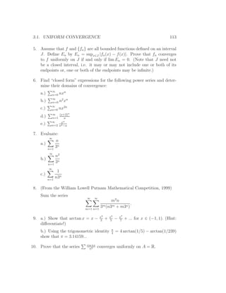
The graph of f4 is shown in figure 3.1.1a and the graph of f is shown
in figure 3.1.1b. Notice that the functions fn are continuous while f is not,
and yet lim fn = f pointwise on [−1, 1]. This example shows that pointwise
limits do not necessarily behave well with respect to continuity.
1
f
4
0.5
-1 -0.75 -0.5 -0.25 0.25 0.5 0.75 1
x
-1
figure 3.1.1a](https://image.slidesharecdn.com/sands807-120904062116-phpapp02/85/Sands807-108-320.jpg)
![3.1. UNIFORM CONVERGENCE 105
1
y f
0.5
-1 -0.75 -0.5 -0.25 0.25 0.5 0.75 1
x
-0.5
-1
figure 3.1.1b
Example 3.1.4
Let
1
2n2 x,
0 ≤ x < 2n
1 1
fn (x) = 2n − 2n2 x, 2n ≤ x < n
1
0, ≤x≤1
n
and let
f (x) = 0, 0 ≤ x ≤ 1.
The graphs of the first three functions of the sequence are shown in figure
1
3.1.2. Notice that 0 fn (x)dx = 1/2 since the graph of fn is a triangle with
1
height n and base 1/n. On the other hand 0 f (x)dx = 0 even though
lim fn = f pointwise on [0, 1]. This shows that pointwise limits do not
necessarily behave well with respect to integration.
The above two examples are meant to convince you that pointwise limits
do not interact well with the concepts of calculus. The reason for this is
that calculus ideas depend on how a function behaves nearby a point, yet
the pointwise limit depends only on the values of the functions at each point
independently. In this chapter we introduce a stronger form of convergence,
uniform convergence, which interacts well with the concepts of calculus.](https://image.slidesharecdn.com/sands807-120904062116-phpapp02/85/Sands807-109-320.jpg)


![108 CHAPTER 3. SEQUENCES AND SERIES OF FUNCTIONS
Definition 3.1.7
∞
The series of functions n=1 fn converges uniformly to f on A if the
sequence of partial sums sn = n fj converges uniformly to f on A.
j=1
Proposition 3.1.8 (Weierstrass M-test)
Let fn be a series of functions and Mn a summable sequence of positive
real numbers with |fn (x)| ≤ Mn for each x ∈ A. Then fn converges
uniformly on A.
Proof: First, let’s notice that the series converges pointwise since if we fix
x in A then, since |fn (x)| ≤ Mn , the comparison test tells that fn (x)
∞
converges absolutely. Let f (x) denote the value of n=1 fn (x), for each
x ∈ A, so f is a function defined on A and fn converges to f pointwise on
A.
Now we wish to show that this convergence is in fact uniform. Let ǫ > 0
be given. Since Mn converges, we can find N ∈ N so that ∞ +1 Mn < ǫ.
n=N
Then for all x ∈ A we have
N ∞
|f (x) − fn (x)| = | fn (x)| (3.1)
n=1 n=N +1
∞
≤ |fn (x)|
n=N +1
∞
≤ Mn
n=N +1
< ǫ.
∞
Thus n=1 fn converges uniformly to f .
As a direct corollary of this and Proposition 2.4.3 we have the following:
Proposition 3.1.9
Let the power series an xn have radius of convergence given by R > 0.
Then, for any c with 0 < c < R, this sum converges uniformly on the interval
[−c, c].
Proof: From Proposition 2.4.3 we know that |an cn | converges. Let Mn =
n n
|an c | and notice that |an x | ≤ Mn for x ∈ [−c, c]. Applying the M-test we
get the desired result.](https://image.slidesharecdn.com/sands807-120904062116-phpapp02/85/Sands807-112-320.jpg)
![3.1. UNIFORM CONVERGENCE 109
Example 3.1.10
Since we know that the geometric series ∞ xn converges to 1−x on
n=0
1
(−1, 1), we can conclude that this convergence is uniform on any subinterval
[−c, c], with 0 ≤ c < 1.
We can now prove the three main theorems which demonstrate the com-
patibility of uniform convergence with the concepts of calculus.
Theorem 3.1.11
Suppose that {fn } is a sequence of continuous functions on the interval
[a, b] and suppose that {fn } converges uniformly on [a, b] to a function f .
Then f is continuous on [a, b].
Proof: Let x0 ∈ [a, b], and ǫ > 0 be given. In order to prove that f is
continuous at x0 we must show how to find δ > 0 so that for all x ∈ [a, b],
with |x − x0 | < δ, we have that |f (x) − f (x0 )| < ǫ.
Now, since we assume that the sequence {fn } converges uniformly to f
on [a, b], we can find an n ∈ N so that |f (x) − fn (x)| < ǫ/3, for all x ∈ [a, b].
(In particular, notice that |f (x0 ) − fn (x0 )| < ǫ/3.)
Also, since we are assuming that the function fn is continuous, we can
choose δ > 0 so that for every x ∈ [a, b] with |x − xo | < δ, we have that
|fn (x) − fn (x0 )| < ǫ/3.
Thus, using the old trick of adding zero (twice), we see that if x ∈ [a, b]
with |x − x0 | < δ, we have
|f (x) − f (x0 )| = |f (x) − fn (x) + fn (x) − fn (x0 ) + fn (x0 ) − f (x0 )|
≤ |f (x) − fn (x)| + |fn (x) − fn (x0 )| + |fn (x0 ) − f (x0 )|
≤ ǫ/3 + ǫ/3 + ǫ/3
≤ ǫ.
Remark: It is worth noting in this proof that once ǫ is given, we choose
a particular fn which gives the necessary inequality, and then we use the
continuity of that particular function. We do not need the full statement of
uniform convergence (the ”for every n > N” part) for this proof.
Theorem 3.1.12
Suppose that {fn } is a sequence of functions that are integrable on the
interval [a, b] and suppose that {fn } converges uniformly on [a, b] to a function](https://image.slidesharecdn.com/sands807-120904062116-phpapp02/85/Sands807-113-320.jpg)
![110 CHAPTER 3. SEQUENCES AND SERIES OF FUNCTIONS
f which is also integrable on [a, b]. Then
b b
lim fn (x)dx = f (x)dx.
n→∞ a a
b b
Proof: Let cn = a fn (x)dx and let c = a f (x)dx. Also, let ǫ > 0 be given.
We need to show that we can find N ∈ N so that |cn − c| < ǫ, for all n > N.
Now, since {fn } converges uniformly to f on [a, b], we can choose N ∈ N so
that |fn (x) − f (x)| < ǫ/(b − a) for all n > N and all x ∈ [a, b]. Thus
b b
|cn − c| = fn (x)dx − f (x)dx
a a
b
= (fn (x) − f (x))dx
a
b
≤ |fn (x) − f (x)|dx
a
b
ǫ
≤ dx
a b−a
≤ǫ
for all n > N.
Theorem 3.1.13
Suppose that {fn } is a sequence of functions which are differentiable on
′
the interval [a, b]. Assume that the derivatives fn are integrable and suppose
that {fn } converges pointwise to a function f on [a, b]. Assume, moreover,
′
that the sequence of derivatives {fn } converges uniformly on [a, b] to some
continuous function g. Then f is differentiable and f ′ (x) = g(x).
′
Proof: Let x be an element of [a, b]. Since the sequence {fn } converges
uniformly to g on the interval [a, b], it also does on the subinterval [a, x].
Also note that since g is continuous on [a, b], it is integrable on that interval.
Thus we can apply the above theorem to get
x x
′
lim fn (t)dt = g(t)dt.
n→∞ a a
x ′
The fundamental theorem of calculus says that a
fn (t)dt = fn (x)−fn (a),
hence, we have
x
g(t)dt = lim (fn (x) − fn (a)),
a n→∞](https://image.slidesharecdn.com/sands807-120904062116-phpapp02/85/Sands807-114-320.jpg)
![3.1. UNIFORM CONVERGENCE 111
but the right hand side of this expression is just f (x) − f (a) since {fn } limits
to f pointwise. Therefore, we have shown that
x
g(t)dt = f (x) − f (a).
a
Since g is assumed continuous, it also follows from the fundamental the-
orem of calculus, then, that f is differentiable and that f ′ (x) = g(x).
Remark: A much stronger version of this theorem is true in which the
continuity of g is not assumed nor the pointwise convergence of {fn } (except
at a single point). The proof is quite a bit trickier, and we don’t need the
general result for our purposes. The interested student can find the result in
Principles of Mathematical Analysis, by W. Rudin.
Applying the above results (along with exercise 11) to power series, we
get:
Theorem 3.1.14
∞
Suppose that the power series f (x) = n=1 an xn has radius of conver-
∞ n−1
gence given by R > 0. Then the power series g(x) = n=1 nan x has
radius of convergence equal to R, f (x) is differentiable on (−R, R), and
f ′ (x) = g(x) for x ∈ (−R, R).
Theorem 3.1.15
Suppose that the power series f (x) = ∞ an xn has radius of conver-
n=1
n+1
gence given by R > 0. Then the power series h(x) = ∞ an x n=1 n+1 also has
radius of convergence equal to R, f (x) is integrable on [a, b], for any closed
interval [a, b] ⊂ (−R, R), and
x
h(x) = f (s)ds
0
for x ∈ (−R, R).
Example 3.1.16
a.) Since we know that ∞ xn = 1−x when −1 < x < 1, we can use
n=0
1
Theorem 3.1.14 to conclude that ∞ nxn−1 = (1−x)2 when −1 < x < 1.
n=0
1
n+1
b.) Applying Theorem 3.1.15 to the same series tells us that ∞ x
n=0 n+1
x ds
converges to 0 1−s = − ln(1 − x) when −1 < x < 1. By re-labeling the](https://image.slidesharecdn.com/sands807-120904062116-phpapp02/85/Sands807-115-320.jpg)
![112 CHAPTER 3. SEQUENCES AND SERIES OF FUNCTIONS
index, we see that
∞
xn
= − ln(1 − x)
n=1
n
for −1 < x < 1. Notice that even though the series converges at x = −1, the
theorem does not tell us anything about what it converges to. On the other
hand, we know from exercise 2.3.11 that the alternating harmonic series
converges to ln(1/2) so the above equality is indeed true on the interval
[−1, 1).
EXERCISES 3.1
1. Prove that the sequence of functions in example 3.1.3 does not converge
uniformly on [−1, 1].
2. Prove that the sequence of functions in example 3.1.4 does not converge
uniformly on [0, 1].
1
3. Let fn (x) = n sin(n2 x). Show that {fn (x)} converges to 0 uniformly on
′
[−1, 1] but that lim fn (x) does not always exist. Explain how this relates
to Theorem 3.1.13.
4. For each of the following sequences of functions {fn } defined on the
given interval J, determine if the sequence converges pointwise to a limit
function f . If the sequence does converge pointwise, determine whether
the convergence is uniform.
x
a.) fn (x) = x+n
, J = [0, ∞).
nx
b.) fn (x) = 1+n2 x2
, J = (−∞, ∞).
xn
c.) fn (x) = 1+xn
, J = [0, ∞).
d.) fn (x) = arctan(nx), J = (−∞, ∞).
e.) fn (x) = e−nx , J = [0, ∞).
f.) fn (x) = e−nx , J = [1, ∞).
g.) fn (x) = xe−nx , J = (−∞, ∞).
h.) fn (x) = x2 e−nx , J = [0, ∞).](https://image.slidesharecdn.com/sands807-120904062116-phpapp02/85/Sands807-116-320.jpg)
![114 CHAPTER 3. SEQUENCES AND SERIES OF FUNCTIONS
∞
1
11. Prove that the series converges uniformly on any interval of the
n=1
nx
form [α, ∞] with α a real number greater than 1. The function defined
by
∞
1
ζ(x) =
n=1
nx
is called the Riemann zeta function.
12. a.) Suppose that the power series f (x) = an xn has radius of con-
vergence R > 0. Use Proposition 3.1.14 to show that the nth -derivative
f (n) (0) is given by n!an .
b.) Use part a.) to find f (10) (0) for f (x) = 1/(1 − x).
13. Prove that the two power series an xn and nan xn have the same
radii of convergence. (Hint: It is easy to show that if |nan cn | converges
then so must |an cn | converge. The other direction needs a comparison
argument similar to that in the proof of Proposition 2.4.3.)
3.2 Taylor Series
In exercise 3.1.12 we saw that if f (x) = ∞ an xn then the coefficient, an ,
n=1
is intimately related to the value of the nth derivative of f at zero, namely
f (n) (0) = n!an .
(Here we should mention the convention that 0! = 1.) The above observation
leads to a method of constructing a power series which might converge to a
given function f . In particular, if the series ∞ an xn has any chance of
n=1
converging to f (x), then the coefficients must be given by
f (n) (0)
an = .
n!
This leads to the following:](https://image.slidesharecdn.com/sands807-120904062116-phpapp02/85/Sands807-118-320.jpg)


![3.2. TAYLOR SERIES 119
for m = 0, 1, . . . , n. In particular, we have that
lim (f (x) − p(x)) = 0.
x→0
By continuity, we conclude that f (0) = p(0) = a0 . Next, apply L’Hˆpital’so
rule to
f (x) − p(x)
lim =0
x→0 x
to conclude that f ′ (0) = p′ (0) = a1 . This result allows us to apply L’Hˆpital’s
o
rule twice to
f (x) − p(x)
lim =0
x→0 x2
to conclude f ′′ (0) = p′′ (0) = 2a2 . Continuing in this fashion (by induction if
you insist on being pedantic), we can conclude f (m) (0) = p(m) (0) = m!am for
f
m = 1, 2, . . . , n, i.e. p = Pn .
A Further Remark: A few moments thought should be given to understand
that in the above proof, we use continuity of the first n − 1 derivatives of
f − p, but we are not assuming that the nth derivative is continuous at 0.
f
The uniqueness of Pn in the above theorem is often useful in determining
Taylor polynomials. To prove that a given nth degree polynomial is the Taylor
polynomial for f , we simply need to show that it agrees with f to order n at
0. To make use of this idea, we need to introduce a little notation:
If P (x) = a0 + a1 x + a2 x2 + · · · + an xn is a polynomial, and 0 ≤ k ≤ n we
define [P ]k to be the degree k polynomial given by truncating P after the xk
term, i.e.
[P ]k (x) = a0 + a1 x + a2 x2 + · · · + ak xk .
For example, if P (x) = 3−x+4x2 +7x4 −4x5 , then [P ]4 (x) = 3−x+4x2 +7x4 ,
while [P ]3 (x) = [P ]2 (x) = 3 − x + 4x2 . Notice that if P and Q are two
polynomials, then [P + Q]k = [P ]k + [Q]k .
Using the uniqueness from the above theorem, it is not too hard to prove
the following:
Theorem 3.2.6
Let f and g be real valued functions defined on a neighborhood of 0 which
have n derivatives at 0. Then
1.) Pn +g = Pn + Pn .
f f g
fg f g
2.) Pn = [Pn Pn ]n .
3.) and if g(0) = 0, then Pn ◦g = [Pn ◦ Pn ]n .
f f g](https://image.slidesharecdn.com/sands807-120904062116-phpapp02/85/Sands807-123-320.jpg)
![120 CHAPTER 3. SEQUENCES AND SERIES OF FUNCTIONS
f ′
4.) Pn−1 = (Pn )′ .
f
x h x f
5.) Let h(x) = 0 f (t) dt, then Pn (x) = 0
Pn−1 (t) dt.
Remark: As a special case of item 3.), one also has
1/(1−g)
4.) if g(0) = 0, then Pn = [1 + Pn + (Pn )2 + · · · + (Pn )n ]n .
g g g
Example 3.2.7
We know that the fifth degree Taylor polynomial for cos(x) is
cos x2 x4
P5 (x) = 1 − +
2 4!
and the fifth degree Taylor polynomial for sin(x) is
sin x3 x5
P5 (x) = x − + ,
3! 5!
so from the above theorem, we can conclude that the fifth degree Taylor
polynomial for sin(x) + cos(x) is
cos(x)+sin(x) x2 x3 x4 x5
P5 =1+x− − + +
2 3! 4! 5!
while the fifth degree Taylor polynomial for the product, cos(x) sin(x), is
given by
cos(x) sin(x) x2 x4 x3 x5
P5 (x) = (1 − + )(x − + )
2 4! 3! 5! 5
x3 x5 x3 x5 x5
=x− + − + +
3! 5! 2 2 · 3! 4!
4x3 16x5
=x− + .
3! 5!
Remark: On the other hand, using the composition rule, we can see that
the fifth degree Taylor polynomial for sin(2x)/2 is given by
sin(2x)/2 1 (2x)3 (2x)5
P5 = (2x) − +
2 3! 5!
3 5
4x 16x
=x− + ,
3! 5!
the same as above.](https://image.slidesharecdn.com/sands807-120904062116-phpapp02/85/Sands807-124-320.jpg)
![3.2. TAYLOR SERIES 121
Example 3.2.8
Setting h(x) = e1−cos(x) we have
2 3
h x2 x4 1 x2 x4 1 x2 x4
P5 (x) = 1 + − + − + − (3.3)
2 24 2 2 24 6 2 24
5
2 4 4 2 4 5
1 x x 1 x x
+ − + −
24 2 24 120 2 24
5
2 4 2 4 2
x x 1 x x
= 1+ − + −
2 24 2 2 24
5
2 4
x x
=1+ + ,
2 12
x
and if k(x) = 0
h(t) dt, we have
x
k h x3 x5
P5 (x) = P4 (t) dt = x + + .
0 6 60
Notice that we have used Theorem 3.2.5 to compute Taylor polynomials of
complicated functions without explicitly computing their derivatives. Thus,
we can now use the fundamental relation an = f (n) (0)/n! to compute values
of f (n) (0) = n!an . In particular, for h(x) in the above example we have that
a0 = 1, a1 = 0, a2 = 1/2, a3 = 0, a4 = 1/12, and a5 = 0, so we see that
h′ (0) = 0, h′′ (0) = 1, h(3) (0) = 0, h(4) (0) = 2, and h(5) (0) = 0. The reader
may find it amusing to check these values by explicitly computing the fifth
derivative of h(x).
f
Theorem 3.2.4 tells us how well Pn approximates f at the point x = 0. To
f
understand whether the sequence of Taylor polynomials {Pn } converges to
f in a neighborhood of zero we need more explicit control on the differences
f
|f (x) − Pn (x)|. The next theorem gives us that control.
Theorem 3.2.9 (Taylor’s Theorem)
Suppose that f, f ′ , f ′′ , ..., f (n+1) are all defined on the interval [0, x]. Let
f
Rn (x) be defined by
f f
Rn (x) = f (x) − Pn (x)
f ′′ (0) 2 f (n) (0) n
= f (x) − f (0) + f ′ (0)x + x + ... + x .
2 n!](https://image.slidesharecdn.com/sands807-120904062116-phpapp02/85/Sands807-125-320.jpg)
![122 CHAPTER 3. SEQUENCES AND SERIES OF FUNCTIONS
Then
f f (n+1) (t) n+1
Rn (x) = x , for some t ∈ (0, x).
(n + 1)!
Example 3.2.10
n
The series ∞ x converges uniformly to ex on any closed interval [a, b].
n=0 n!
To prove this, first notice that the radius of convergence for this series is
infinite, so we know the series converges uniformly on any closed interval. In
particular, we know that for any given x,
lim xn /n! = 0.
n→∞
Now we need only show that the series converges to ex pointwise. Fix some
j
x ∈ R and let Pn (x) = n x , then Taylor’s Theorem tells us that
j=0 j!
|ex − Pn (x)| = et |x|n+1 /(n + 1)!
for some t between 0 and x. But then et < e|x| so we get
e|x| |x|n+1
|ex − Pn (x)| ≤ .
(n + 1)!
We have remarked above that the sequence |x|n /n! converges to zero as n
goes to infinity, so, given ǫ > 0, we can choose N so large that |x|n+1 /n + 1! <
e−|x| ǫ for all n > N. Then, for all n > N, we have that |ex − Pn (x)| < ǫ.
Thus Pn (x) converges to ex .
Another valuable application of Taylor’s Theorem is that it gives us esti-
mates on how well a Taylor polynomial approximates the original function.
Example 3.2.11
As above, the nth Taylor polynomial for f (x) = ex is given by Pn (x) =
f
n j
j=0 x /j! and Taylor’s Theorem gives us an estimate for the error term
f
|f (x) − Pn (x)|. Let’s use this to find a decimal approximation for f (1) = e
which is correct to 4 decimal places. To do this, we must figure out which n
will give us a small enough error. By Taylor’s Theorem, we have
f f (n+1) (t) n f (n+1) (t)
|e − Pn (1)| ≤ (1) =
(n + 1)! (n + 1)!](https://image.slidesharecdn.com/sands807-120904062116-phpapp02/85/Sands807-126-320.jpg)

![124 CHAPTER 3. SEQUENCES AND SERIES OF FUNCTIONS
2. Find the Taylor series centred at a for f (x) = 1 + x + x2 + x3 when
(a) a = 0 (b) a = 1 (c) a = 2
∞ n x2n
3. Prove that the series n=0 (−1) (2n)! converges uniformly to cos x on any
closed interval [a, b].
4. Find the sum of these series
∞ ∞ ∞
x4n π 2n xn
(a) (−1)n (b) (−1)n (c)
n=0
n! n=0
62n (2n)! n=0
2n (n + 1)!
5. Use the 5th degree Taylor polynomial for f (x) = ex and Taylor’s theorem
to obtain the estimate
1957 1956
≤e≤
720 719
6. For what values of x do the following polynomials approximate sin x to
within 0.01
(a) P1 (x) = x (b) P3 (x) = x − x3 /6 (c) P5 (x) = x − x3 /6 + x5 /120
7. How accurately does 1+x+x2 /2 approximate ex for x ∈ [−1, 1]? Can you
find a polynomial that approximates ex to within 0.001 on this interval?
8. Use Taylor’s Theorem to approximate cos(π/4) to 5 decimal places.
9. Find the Taylor series for x2 sin(x2 ).
10. Find the 10th degree Taylor polynomial for the following functions:
a.) cos(x2 )
b.) sin(2x)
c.) ex+1
2
d.) ex cos(x3 )
sin(x2 )
e.) 1+x2
1−cos(x6 )
11. a.) Find the Taylor series for f (x) = x12
.
b.) Use part a.) to determine f (n) (0) for n = 0, 1, 2, 3, ..., 12.](https://image.slidesharecdn.com/sands807-120904062116-phpapp02/85/Sands807-128-320.jpg)


The document is an introduction to sequences and series. It begins by defining sequences and providing examples of sequences, including coin tosses, picking marbles from a bag, and Harry the Hare walking to the grocery store. It then discusses different ways to represent sequences, such as listing terms explicitly or using notation like {ai}. The document also describes different ways to define a sequence, including using an explicit formula for the nth term, listing the first few terms, or using a recursive formula relating terms. It concludes by introducing arithmetic and geometric sequences as important families of sequences.