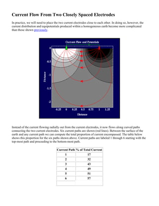
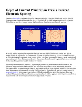
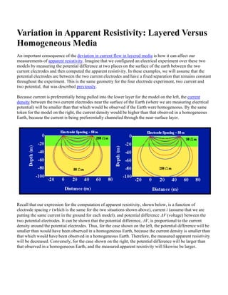
SlideShare a Scribd company logo
1 of 47
Download to read offline
This home page introduces a prototype of a new educational program being developed with the support of the Society of Exploration
Geophysicists. It is currently under development and will be changing almost daily.
The SEG welcomes feedback on the educational concept and the effectiveness of these prototype modules. It especially encourages earth-
science educators to use this program as a means of becoming involved in the broader issue of providing conceptual, cross-disciplinary
learning that will enable people from all disciplines to be more-effective members of earth-science teams. Feel free to contact:
Tom Boyd (project leader) tboyd@mines.edu tel:303-273-3522 fax: 303-273-3478
Copyright (c) Thomas M. Boyd, 1996 - 1999 All rights reserved.
All files including but not limited to HTML, Java, Javascript, C, Shell scripts, and Pearl scripts, included in this site (subdirectory
/csminfo/htdocs/fs_home/tboyd/GP311) are not distributed as public domain software, but are freely available under the following
license.
Definition
Resistivity Method - Observation of electric fields
caused by current introduced into the ground as a
means of studying earth resistivity in geophysical
exploration. Resistivity is the property of a material
that resists the flow of electrical current.*
Useful References
• Burger, H. R., Exploration Geophysics of the
Shallow Subsurface, Prentice Hall P T R,
1992.
• Robinson, E. S., and C. Coruh, Basic
Exploration Geophysics, John Wiley, 1988.
• Telford, W. M., L. P. Geldart, and R. E.
Sheriff, Applied Geophysics, 2nd ed.,
Cambridge University Press, 1990.
Return to the Introduction to Geophysical Exploration
Homepage
*Definition from the Encyclopedic Dictionary of Exploration Geophysics by R. E. Sheriff, published by
the Society of Exploration Geophysicists.
Note Outline: Geophysical Surveying Using DC
Resistivity
Introduction
• Active and Passive Geophysical Methods
• Advantages and Disadvantages of Each Method
• Electrical Methods Overview
Resistivity Basics
• Current Flow and Ohm's Law
• The Fundamental Electrical Property is Resistivity, NOT Resistance
• Resistivities for Common Earth Materials
• Current Density and Electric Field
• A First Estimate of Resistivity
• Current Flow From Two Closely Spaced Electrodes
• A Practical Way of Measuring Resistivity
Resistivity Surveys and Geology
• Sources of Noise
• Depth of Current Penetration Versus Current Electrode Spacing
• Current Flow in Layered Media
• Variation in Apparent Resistivity: Layered Versus Homogeneous Media
• Current Flow in Layered Media Versus Electrode Spacing
• A Second Example of Current Flow in Layered Media
Resistivity Equipment and Field Procedures
• Equipment
• Survey Types Overview: Soundings and Profiles
• Soundings: Wenner and Schlumberger
• Electrode Spacings and Apparent Resistivity Plots
• Advantages and Disadvantages of Each Survey Type
• Profiles
Interpretation of Resistivity Measurements
• Apparent Resistivity Curves for Soundings Over One-Layered Media
• Apparent Resistivity Curves for One-Layered Media: Part 2
• Apparent Resistivity Curves in Two-Layered Media
• Two-Layered Media: Another Example
Geophysical Surveys: Active Versus Passive
Geophysical surveys can be classified into one of two types: Active and Passive.
• Passive geophysical surveys incorporate measurements of naturally occurring fields or properties of
the earth. We have already considered passive geophysical surveys in our discussions of gravity and
magnetic surveys. In these two cases, the naturally occurring fields are the gravitational and
magnetic fields. We simply measure spatial variations in these fields in an attempt to infer
something about the subsurface geology. The fields and properties that we are measuring in this
class of experiments exist regardless of our geophysical survey. Examples of other earth properties
that could be passively measured include radiometric decay products, certain electrical fields, and
certain electro-magnetic fields.
• In conducting active geophysical surveys, on the other hand, a signal is injected into the earth and
we then measure how the earth responds to this signal. These signals could take a variety of forms
such as displacement, an electrical current, or an active radiometric source. The final two survey
methods considered in this short course, DC resistivity and seismic refraction, are examples of active
geophysical experiments.
Active and passive geophysical surveys each have their own set of advantages and disadvantages.
Advantages and Disadvantages of Active and
Passive Experiments
Shown below is a table listing some of the advantages and disadvantages to both active and passive surveys.
In reading these, please note that the terms passive and active cover a wide range of geophysical survey
methods. Thus, the listed advantages and disadvantages are by necessity generalized and might not apply to
any given specific survey.
Active Passive
Advantage Disadvantage Advantage Disadvantage
Better control of noise
sources through control
of injected signal.
Because both sources and
receivers are under the
surveyor's control, he must
supply both. Therefore,
field equipment tends to be
more complex.
Surveyor need only
record a naturally
occurring field;
therefore, he need
supply only a sensor
and a data recorder.
Less control of noise
because source of the
signal is out of the
control of the surveyor.
Because propagating
fields are generally
measured, active
experiments usually
provide better depth
control over source of
anomalous signal.
Field operations and
logistics are generally more
complex and time
consuming than passive
experiments.
Field operations are
generally very time
efficient. Thus,
passive experiments
can be run over wider
areas in a more cost-
effective manner.
Because passive fields
are generally the result
of integrating
anomalous geologic
contributions over
wide areas,
identification of the
source of an anomalous
reading can be
difficult.
Many different
source/receiver
configurations can be
used allowing for a wide
variety of survey
designs. This allows
survey designers great
flexibility in customizing
surveys for particular
problems.
Many different
source/receiver
configurations can be used
allowing for a wide variety
of survey designs. The
increase in the number of
field options inevitably
leads to greater survey
design costs and potentially
to increased probability of
field mishaps.
One or two well-
established field
procedures are
generally used.
Contractors can
provide these surveys
on short notice with
relatively easily
quantifiable results.
One or two well-
established field
procedures is generally
used. This limits the
amount of
customization that can
be done for specific
problems.
Once set up, active
experiments are capable
of producing vast
quantities of data that
can be used to interpret
subtle details of the
earth's subsurface.
The large quantity of data
obtained in many active
experiments can become
overwhelming to process
and interpret.
Interpretation of the
limited set of
observations can be
accomplished with
modest computational
requirements quickly
and efficiently.
The data sets collected
in passive experiments
are smaller than those
collected in active
experiments and
usually do not allow for
as detailed an
interpretation.
Electrical Methods Overview
Bridging our subdivision of geophysical techniques into passive and active methods are the electrical and
electromagnetic methods. Taken as a whole, the electrical and electromagnetic methods represent the largest
class of all geophysical methods, some passively monitor natural signals while others employ active
sources.
In addition to their great variety, this group of geophysical techniques represents
some of the oldest means of exploring the Earth's interior. For example, the SP
method described below dates back to the 1830's when it was used in Cornwall,
England by Robert Fox to find extensions of known copper deposits. Natural
electrical currents in the Earth, referred to as telluric currents, were first identified
by Peter Barlow (pictured) in 1847. The EM method was developed in the 1920's
for the exploration of base-metal deposits.
Electrical methods employ a variety of measurements of the effects of electrical
current flow within the Earth. The phenomena that can be measured include current
flow, electrical potential (voltages), and electromagnetic fields. A summary of the
more well-known electrical methods is given below. In this set of notes we will
consider only one of these methods, the DC resistivity method.
• DC Resistivity - This is an active method that employs measurements of electrical potential
associated with subsurface electrical current flow generated by a DC, or slowly varying AC, source.
Factors that affect the measured potential, and thus can be mapped using this method, include the
presence and quality of pore fluids and clays. Our discussions will focus solely on this method.
• Induced Polarization (IP) - This is an active method that is commonly done in conjunction with DC
Resistivity. It employs measurements of the transient (short-term) variations in potential as the
current is initially applied or removed from the ground. It has been observed that when a current is
applied to the ground, the ground behaves much like a capacitor, storing some of the applied current
as a charge that is dissipated upon removal of the current. In this process, both capacitive and
electrochemical effects are responsible. IP is commonly used to detect concentrations of clay and
electrically conductive metallic mineral grains.
• Self Potential (SP) - This is a passive method that employs measurements of naturally occurring
electrical potentials commonly associated with the weathering of sulfide ore bodies. Measurable
electrical potentials have also been observed in association with ground-water flow and certain
biologic processes. The only equipment needed for conducting an SP survey is a high-impedence
voltmeter and some means of making good electrical contact with the ground.
• Electromagnetic (EM) - This is an active method that employs measurements of a time-varying
magnetic field generated by induction through current flow within the earth. In this technique, a
time-varying magnetic field is generated at the surface of the earth that produces a time-varying
electrical current in the earth through induction. A receiver is deployed that compares the magnetic
field produced by the current-flow in the earth to that generated at the source. EM is used for
locating conductive base-metal deposits, for locating buried pipes and cables, for the detection of
unexploded ordnance, and for near-surface geophysical mapping.
• Magnetotelluric (MT) - This is a passive method that employs measurements of naturally occurring
electrical currents, or telluric currents, generated by magnetic induction of electrical currents in the
ionosphere. This method can be used to determine electrical properties of materials at relatively
great depths (down to and including the mantle) inside the Earth. In this technique, a time variation
in electrical potential is measured at a base station and at survey stations. Differences in the recorded
signal are used to estimate subsurface distribution of electrical resistivity.
Current Flow and Ohm's Law
In 1827, Georg Ohm defined an empirical relationship between the current flowing
through a wire and the voltage potential required to drive that current.*
Ohm found that the current, I, was proportional to the voltage, V, for a broad class of
materials that we now refer to as ohmic materials. The constant of proportionality is
called the resistance of the material and has the units of voltage (volts) over current
(amperes), or ohms.
In principle, it is relatively simple to measure the resistance of a strand of wire. Connect a battery to a wire
of known voltage and then measure the current flowing through the wire. The voltage divided by the current
yields the resistance of the wire. In essence, this is how your multimeter measures resistance. In making this
measurement, however, we must ask two crucial questions.
• How is the measured resistance related to some fundamental property of the material from which the
wire is made?
• How can we apply this relatively simple experiment to determine electrical properties of earth
materials?
*Ohm actually stated his law in terms of current density and electrical field. We will describe these
properties later. For one-dimensional current flow in a wire, his law is given as described above.
It's Resistivity, NOT Resistance
The problem with using resistance as a measurement is that it depends not only on the material from which
the wire is made, but also the geometry of the wire. If we were to increase the length of wire, for example,
the measured resistance would increase. Also, if we were to decrease the diameter of the wire, the measured
resistance would increase. We want to define a property that describes a material's ability to transmit
electrical current that is independent of the geometrical factors.
The geometrically-independent quantity that is used is called resistivity and is usually indicated by the
Greek symbol ρ*.
In the case of a wire, resistivity is defined as the resistance in the wire, times the cross-sectional area of the
wire, divided by the length of the wire. The units associated with resistivity are thus, ohm - m (ohm -
meters).
Resistivity is a fundamental parameter of the material making up the wire that describes how easily the wire
can transmit an electrical current. High values of resistivity imply that the material making up the wire is
very resistant to the flow of electricity. Low values of resistivity imply that the material making up the wire
transmits electricial current very easily.
*Unfortunately, the symbol ρ is used throughout the geophysical literature to represent both density and
resistivity. Although one would suspect that this could lead to some confusion, it rarely does because the
context in which ρ is used will usually define whether it is representing density or resistivity
unambiguously. In these notes, we will follow standard geophysical practice and use ρ to represent both
physical properties.
Resistivity of Earth Materials
Although some native metals and graphite conduct electricity, most rock-forming minerals are electrical
insulators. Measured resistivities in Earth materials are primarily controlled by the movement of charged
ions in pore fluids. Although water itself is not a good conductor of electricity, ground water generally
contains dissolved compounds that greatly enhance its ability to conduct electricity. Hence, porosity and
fluid saturation tend to dominate electrical resistivity measurements. In addition to pores, fractures within
crystalline rock can lead to low resistivities if they are filled with fluids.
The resistivities of various earth materials are shown below.
Material Resistivity (Ohm-meter)
Air ∞
Pyrite 3 x 10^-1
Galena 2 x 10^-3
Quartz 4 x 10^10 - 2 x 10^14
Calcite 1 x 10^12 - 1 x 10^13
Rock Salt 30 - 1 x 10^13
Mica 9 x 10^12 - 1 x 10^14
Granite 100 - 1 x 10^6
Gabbro 1 x 10^3 - 1 x 10^6
Basalt 10 - 1 x 10^7
Limestones 50 - 1 x 10^7
Sandstones 1 - 1 x 10^8
Shales 20 - 2 x 10^3
Dolomite 100 - 10,000
Sand 1 - 1,000
Clay 1 - 100
Ground Water 0.5 - 300
Sea Water 0.2
Like susceptibilities, there is a large range of resistivities, not only between varying rocks and minerals but
also within rocks of the same type. This range of resistivities, as described above, is primarily a function of
fluid content. Thus, a common target for electrical surveys is the identification of fluid saturated zones. For
example, resistivity methods are commonly used in engineering and environmental studies for the
identification of the water table.
Current Densities and Equipotentials
To describe the nature of electrical current flow in media occupying a volume, we must move beyond our
simple notions of current and voltage gained from our experience with wires, resistors, and batteries. In the
Earth, or any three-dimensional body, electrical current is not constrained to flow along a single path as it
does in a wire. Consider as an example the situation shown below. A battery is connected to the earth by
wires and electrodes at two remote points (that is, the electrical connections to the earth are very distant
from one another). The Earth, not being a perfect insulator, conducts the electrical current imparted by the
battery. At this stage, let's assume the resistivity of the earth is uniform throughout the Earth. How does the
current flow through the Earth?
In this example, current flows (the red lines) out from the electrode (the green square) radially along straight
lines (the second electrode is far to the right of the figure as it is drawn). If we could take a voltmeter and
measure the voltage drop imposed by the resistivity of the medium from a distance very far from the current
electrode to various places in the media, we would find that the voltage drops would be constant along
circular lines centered at the electrode (That is, one of the leads to the voltmeter would have to make contact
with the ground at a distance very far from the electrode, the other is then moved throughout the medium).
These lines are referred to as equipotentials (think equal voltage). In three-dimensions, they form
hemispheres centered on the electrodes. Several equipotential lines are shown in black with the voltage drop
associated by each line shown in gray scale. The darker the gray scale, the smaller the potential drop
between this location and a location very far from the current electrode.
Voltage differences between any two points in the medium can be computed by simply subtracting the
potentials at the two points. Thus, if the two points line on a hemisphere centered at the current electrode,
there will be no voltage difference recorded, because these two locations lie along an equipotential surface.
That is, if you were to take your voltmeter and connect to two points within the earth that were on the same
equipotential surface, you would read a voltage difference of zero. When compared to the potential near the
electrode, voltage differences will increase away from the electrode. This should make sense, what you are
measuring with your voltmeter is proportional to the current passing through the media times the resistance
of the media as given by Ohm's law. As you move away from the electrode, your current is traveling
through more of the media. The resistance increases as the path increases, hence, the voltage increases.
At any point in the medium, the current density is defined as the amount of current passing through a unit
area of an equipotential surface. Thus, close to the electrode, all of the current is passing through a very
small volume. The current crossing any equipotential surface normalized by the area of the surface will thus
be high. Far away from the electrode, this same current occupies a much larger volume of the medium. The
current crossing any equipontential surface (which is the same regardless of where the surface is in the
volume) normalized by the area of the surface (which is now large) will be small. Current density has the
units of Amperes per meter squared.
A First Estimate of Resistivity
The voltage change from a single current electrode to some point in the
half space representing the earth is given by the expression to the right. In
this expression, V is voltage, I is current, ρ is resistivity, and r is the
distance between the current electrode and the point the voltage is
measured. Notice that this expression is nothing more than Ohm's law
with the resistance, R equal to ρ over 2πr.
If the Earth had a constant resistivity, which it doesn't, we could estimate
this resistivity by performing the following experiment. Attach to a wire
connecting the battery with one of the current electrodes an ammeter to measure the amount of current
going into the earth. Place one electrode connected to a voltmeter next to the current electrode and place the
other at some distance, r, away from the electrode and measure the voltage difference between the two
locations. Using the expression given above, compute the resistivity, ρ.
In practice, this experiment could be difficult to implement because the two current electrodes must be
placed a great (usually 10 times the distance over which the voltage is being measured) distance from one
another. So, why not simply decrease the distance between the two voltage electrodes so the distance
between the two current electrodes remains a practical distance? The problem is that the closer the two
voltage electrodes are to each other, the smaller the voltage difference that must be measured. Thus, there is
a practical limit to how close the two voltage electrodes can be and thereby how close the two current
electrodes can be.
As another note, one may ask why don't we simply attach the voltmeter to the wire in which the current is
flowing and measure the voltage drop between the two current electrodes. In principle, this could be done.
In practice, however, it is difficult to obtain reliable information because what you measure is more a
function of the contact resistance between the earth and the current electrodes than of the resistivity of the
Earth. The contact resistance is the resistance that is encountered by current flow because the electrode does
not make perfect electrical contact with the earth. Contact resistances can be quite large, on the order of
kilo-ohms (10^3 ohms). If a large (infinite) impedance voltmeter is used, however, to make the voltage
measurement across two separate voltage electrodes, little current actually flows through the voltage
electrodes and contact resistance is unimportant to the measurement.
Current Flow From Two Closely Spaced Electrodes
In practice, we will need to place the two current electrodes close to each other. In doing so, however, the
current distribution and equipotentials produced within a homogeneous earth become more complicated
than those shown previously.
Instead of the current flowing radially out from the current electrodes, it now flows along curved paths
connecting the two current electrodes. Six current paths are shown (red lines). Between the surface of the
earth and any current path we can compute the total proportion of current encompassed. The table below
shows this proportion for the six paths shown above. Current paths are labeled 1 through 6 starting with the
top-most path and proceeding to the bottom-most path.
Current Path % of Total Current
1 17
2 32
3 43
4 49
5 51
6 57
From these calculations and the graph of the current flow shown above, notice that almost 50% of the
current placed into the ground flows through rock at depths shallower or equal to the current electrode
spacing.
A Practical Way of Measuring Resistivity
Using an experimental configuration where the two current electrodes are placed relatively close to one
another as described previously and using two potential electrodes placed between the two current
electrodes, we can now estimate the resistivity of our homogeneous earth. The configuration of the four
electrodes for this experiment is shown below. Let the distances between the four electrodes be given by r1,
r2, r3, and r4, as shown in the figure.
The potential computed along the surface of the earth is shown in the graph below. The voltage we would
observe with our voltmeter is the difference in potential at the two voltage electrodes, ΔV. The horizontal
positions of the four electrodes, two current (red and green) and two potential (purple), are indicated along
the top of the figure.
Notice, that in this configuration, the voltage recorded by the voltmeter (ΔV) is relatively small. That is, the
difference in the potential at the locations of the two potential electrodes is small. We could increase the
size of the voltage recorded by the voltmeter by moving the two potential electrodes outward, closer to the
two current electrodes. For a variety of reasons, some related to the reduction of noise and some related to
maximizing the depth over which our measurements are sensitive, we will typically not move the potential
and current electrodes close together. Thus, a very sensitive voltmeter must be used. In addition to having a
large impedance, voltmeters need to be able to record voltage differences down to mV (10^-3 volts). If the
potential electrodes were moved closer to the two current electrodes, larger voltages would be recorded. For
a variety of reasons, however, we will typically not do this in the field.
Knowing the locations of the four electrodes, and by measuring the amount of current input into the ground,
i and the voltage difference between the two potential electrodes, ΔV, we can compute the resistivity of the
medium, ρa, using the following equation.
In this particular case, regardless of the location of the four electrodes, ρa will be exactly equal to the
resistivity of the medium. The resistivity computed using the equation given above is referred to as the
apparent resistivity. We call it the apparent resistivity for the following reason. We can always compute ρa,
and we only need to know the locations of the electrodes and measure the current and voltage. If, however,
the Earth does not have a constant resistivity (that is, if the resistivity varies with depth or horizontally), the
resistivity computed by the above equation will not represent the true resistivity of the Earth. Thus, we refer
to it as an apparent resistivity.
As a final caveat, as written above, the difference between the apparent and the true resistivity of the
medium is not a function of any noise that might be associated with the measurements we are attempting to
record. The difference, rather, comes from the fact that our measurement, in some sense, averages the true
resistivities of some region of the earth, yielding an apparent resistivity that may or may not represent the
true resistivity at some point within the earth.
Sources of Noise
Even given the simple experiment outline on the previous page, there are a number of sources of noise that
can affect our measurements of voltage and current
from which we will compute apparent resistivities.
• Electrode Polarization - A metallic electrode,
like a copper or steel rod, in contact with an
electrolyte other than a saturated solution of
one of its own salts, like ground water, will
generate a measurable contact potential. In
applications such as SP, these contact
potentials can be larger than the natural
potential that you are trying to record. Even
for the DC methods described here, these
potentials can be a significant fraction of the
total potential measured.
For DC work, there are two possible solutions.
1. Use nonpolarizing electrodes. These are electrodes that contain a metallic conducting rod in
contact with a saturated solution of its own salt. Copper and copper sulfate solution are
commonly used. The rod and solution are placed in a porous ceramic container that allows
the saturated solution to slowly leak out and make contact with the ground. Because these
solutions are rather environmentally unfriendly, and because the method described below is
easy to employ, these so-called porous pot electrodes are rarely used in DC work. They are,
however, commonly used in SP and IP surveys.
A simple method to avoid the influence of these contact
potentials is to periodically reverse the current flow in the
current electrodes or use a slowly varying, a few cycles
per second, AC current. As the current reverses, the
polarizations at each electrode break down and begin to
reverse. By measuring over several cycles, robust current
and voltage measurements can be made with negligible
polarization effects.
• Telluric Currents -As described previously,
naturally existing currents flow within the earth.
These currents are referred to as telluric currents.
The existance of these currents can generate a measurable voltage across the potential electrodes
even when no current is flowing through the current electrodes. By periodically reversing the current
from the current electrodes, or by employing a slowly varying AC current, the effects of telluric
currents on the measured voltage can be cancelled.
• Presence of Nearby Conductors -Electrical surveys can not be performed around conductors that
make contact with the ground. For example, the presence of buried pipes or chain-linked fences will
act as current sinks. Because of their low resistivity, current will preferentially flow along these
structures rather than flowing through the earth. The presence of these nearby conductors essentially
acts as electrical shorts in the system.
• Low Resistivity at the Near Surface -Just as nearby conductors can act as current sinks that short out
an electrical resistivity experiment, if the very near surface has a low resistivity, it is difficult to get
current to flow more deeply within the earth. Thus, a highly conductive* near-surface layer such as a
perched water table can prevent current from flowing more deeply within the earth.
• Near-Electrode Geology and Topography - Any variations in geology or water content localized
around an electrode that produce near-surface variations in resistivity can greatly influence
resistivity measurements. In addition, rugged topography will act to concentrate current flow in
valleys and disperse current flow on hills.
• Current Induction in Measurement Cables - Current flowing through the cables connecting the
current source to the current electrodes can produce an induced current in the cables connecting the
voltmeter to the voltage electrodes, thereby generating a spurious voltage reading. This source of
noise can be minimized by keeping the current cables physically away from, a meter or two, the
voltage cables.
*Conductivity is the opposite of resistivity. Highly conductive media transmit electrical current with great
ease and thus have a low resistivity. Mathematically, conductivity is the reciprical of resisitivity and is
measured in the units of 1 over Ohm meters. One over Ohm is referred to as a siemen (S). Thus, the units of
conductivity are siemens per meter.
Depth of Current Penetration Versus Current
Electrode Spacing
As shown previously, when two current electrodes are moved in close proximity to one another, current
flows along arc-shaped paths connecting the two electrodes. If the earth has a constant resistivity, about
50% of the current flows through rock at depths shallower than the current electrode spacing.
What this implies is that by increasing the electrode spacing, more of the injected current will flow to
greater depths, as indicated in the figure above. Because the total resistance in the electrical path increases
as electrode spacing is increased, to get current to flow over these longer paths requires a larger generator of
electrical current. Thus, the maximum distance that current electrodes can be separated by is in part dictated
by the size of the generator used to produce the current.
Assuming for a moment that we have a large enough generator to produce a measurable current in the
ground at large current electrode spacings, this increase in the depth of current penetration as current
electrode spacing increases suggests a way in which we could hope to decipher the resistivity structure of an
area. Because current flows mostly near the Earth's surface for close electrode spacings, measurements of
apparent resistivity at these electrode spacings will be dominated by the resistivity structure of the near
surface. If the current and potential electrodes are spread apart and the apparent resistivity remeasured, these
measurements will incorporate information on deeper Earth structure.
Current Flow in Layered Media
How does the presence of depth variations in resistivity affect the flow of electrical current? In the previous
examples, we assumed that the Earth has a constant resistivity. Obviously, this isn't true or else we wouldn't
be trying to map the variation in resistivity throughout the Earth. Although resistivity could conceivably
vary in depth and in horizontal position, we will initially only consider variations in depth. In addition, we
will assume that these depth variations in resistivity can be quantized into a series of discrete layers, each
with a constant resistivity. Thus, initially we will not consider variations in resistivity in the horizontal
direction or continuous variations with depth*.
Shown below are current-flow paths (red) from two current electrodes in two simple two-layer models. The
model to the left contains a high-resistivity layer (250 ohm-m) overlying a lower resistivity layer (50 ohm-
m). This model is characteristic of the resistivity profile that would be found in a region where unsaturated
alluvium overlies water saturated alluvium. The model to the right contains a low-resistivity layer (50 ohm-
m) overlying a higher resistivity layer (250 ohm-m). This model is characteristic of a perched aquifer. For
comparison, we've also shown the paths current would have flowed along if the Earth had a constant
resistivity (blue) equal to that of the top layer. These paths are identical to those described previously.
Notice that the current flow in the layered media deviates from that observed in the homogeneous media. In
particular, notice that in the layered media the current flow lines are distorted in such a way that current
preferentially seems to be attracted to the lower-resistivity portion of the layered media. In the model on the
left, current appears to be pulled downward into the 50 ohm-m layer. In the model on the right, current
appears to be bent upward, trying to remain within the lower resistivity layer at the top of the model. This
shouldn't be surprising. What we are observing is the current's preference toward flowing through the path
of least resistance. For the model on the left, that path is through the deep layer. For the model on the right,
that path is through the shallow layer.
*For all practical purposes, this layered model does allow for continuous variations in resistivity with depth,
because we have made no constraints on the number of layers or their thicknesses allowed in the model.
Thus, a smoothly varying resistivity depth profile could be approximated by a large number of very thin,
constant resistivity layers.
Variation in Apparent Resistivity: Layered Versus
Homogeneous Media
An important consequence of the deviation in current flow in layered media is how it can affect our
measurements of apparent resistivity. Imagine that we configured an electrical experiment over these two
models by measuring the potential difference at two places on the surface of the earth between the two
current electrodes and then computed the apparent resistivity. In these examples, we will assume that the
potential electrodes are between the two current electrodes and have a fixed separation that remains constant
throughout the experiment. This is the same geometry for the four electrode experiment, two current and
two potential, that was described previously.
Because current is preferentially being pulled into the lower layer for the model on the left, the current
density between the two current electrodes near the surface of the Earth (where we are measuring electrical
potential) will be smaller than that which would be observed if the Earth were homogeneous. By the same
token for the model on the right, the current density would be higher than that observed in a homogeneous
Earth, because the current is being preferentially channeled through the near-surface layer.
Recall that our expression for the computation of apparent resistivity, shown below, is a function of
electrode spacing r (which is the same for the two situations shown above), current i (assume that we are
putting the same current in the ground for each model), and potential difference ΔV (voltage) between the
two potential electrodes. It can be shown that the potential difference, ΔV, is proportional to the current
density around the potential electrodes. Thus, for the case shown on the left, the potential difference will be
smaller than would have been observed in a homogeneous Earth, because the current density is smaller than
that which would have been observed in a homogeneous Earth. Therefore, the measured apparent resistivity
will be decreased. Conversely, for the case shown on the right, the potential difference will be larger than
that observed in a homogeneous Earth, and the measured apparent resistivity will likewise be larger.
Current Flow in Layered Media Versus Current
Electrode Spacing
Imagine that we conduct a series of four electrode experiments, each centered about the same point. Let's
assume that the potential electrodes remain centered between the current electrodes and that their separation
is held fixed. Initially, the current electrodes are placed close together and we measure current and voltage
from which we compute apparent resistivity. Then we perform the same experiment, but we systematically
increase the current electrode spacing while holding the potential electrode spacing fixed. What will
happen?
Consider the earth model shown below: a high resistivity layer over a lower resistivity layer.
When the current electrodes are closely spaced, in the region surrounding the potential electrode positions
(between the two current electrodes), most of the current flows through the upper layer along paths that are
close to those that they would have flown along if the model were homogeneous. That is, in this electrode
configuration, current flow is not perturbed enough near the potential electrodes for us to be able to
distinguish between this layered model and a homogeneous Earth model with a resistivity equal to the
resistivity of the top layer. Thus, the computed apparent resistivity will be close to the resistivity of the
upper layer, 250 ohm-m.
Now, we increase the current electrode spacing and repeat the same experiment. At larger current electrode
spacings, the current flow near the potential electrodes is significantly altered by the presence of the
subsurface boundary. In this case, current is preferentially drawn downward into the lower resistivity layer,
decreasing the current density between the two current electrodes where we will measure the voltage with
our two potential electrodes. This decrease in current density will cause our computed value of apparent
resistivity to decrease from 250 ohm-m.
At very large current electrode spacings, underneath our potential electrodes, the pattern of current flow is
again similar to that which we would observe in a homogeneous Earth model. In this case, however, the
media has a resistivity of 50 ohm-m, not 250 ohm-m. Thus, if we were to compute and plot apparent
resistivity for a variety of current electrode spacings while holding the potential electrodes fixed, we would
generate a plot similar to that shown below.
As is common for curves of this type, notice that this plot is a Log-Log plot. Instead of plotting apparent
resistivity versus current electrode spacing, we have plotted the Log (base 10) of the apparent resistivity
versus the Log (base 10) of the current electrode spacing. This is done because, in practice, we will find that
both the apparent resistivities and the current electrode spacings will vary over two to three orders of
magnitude (e.g., spacings can commonly increase from 0.25 m to 250 m). Using Log-Log plots provides us
with a means of compressing the relevant information into a single graph. In the example shown above,
notice that the apparent resistivity does not approach the resistivity of the lower layer until the electrode
spacing approaches 500 m! Thus, large electrode spacings are required to see deep structure. A good rule of
thumb is that you will need current electrode spacings on the order of 10 times the depth to which you
would like to see.
A Second Example of Current Flow in Layered
Media
As another example of current flow in layered media and how apparent resistivity can vary with varying
electrode spacing*, consider the earth model shown below. In this case, a low resistivity layer overlies a
higher resistivity halfspace.
Initially with the current electrodes closely spaced, most of the current is confined to the upper layer along
paths that are very close to those that they would have assumed if the model were homogeneous. The
computed apparent resistivity is very close to the resistivity of the upper layer, 50 ohm-m.
At larger current electrode spacings, more current flows to greater depths. Between the two current
electrodes, where the potential electrodes are located, the current flow lines become significantly distorted
by the presence of the higher-resistivity layer located at depth. Therefore, around the potential electrodes the
current density is larger than we would have observed in a homogeneous Earth. This relative increase in
current density will cause our computed value of apparent resistivity to increase from 50 ohm-m.
At very large current electrode spacings, current flow around our potential electrodes again approximates
that which we would observe in a homogeneous Earth. In this case, however, because most of the current is
flowing through the lower media in the vicinity of the potential electrodes, the computed resistivity we be
close to 250 ohm-m. Thus, as current electrode spacing is increased, the apparent resistivity will increase,
eventually approaching 250 ohm-m. A plot of apparent resistivity versus current electrode spacing is shown
below.
Because current would prefer to flow within the first layer, notice that the apparent resistivity approaches
the resistivity of the halfspace more slowly (i.e., with greater electrode spacings) than was found in the
previous case.
*Although we have not explicitly said this, the relevant spacing in the phrase electrode spacing is not the
spacing between the current electrodes or the spacing between the potential electrodes but rather the spacing
between the current and the potential electrodes. Thus, even if our current electrode spacing is large (so that
most or our current is flowing through the lower medium), if our potential electrodes are close to the current
electrodes, we will compute apparent resistivities that are more like the resistivity of the upper layer than
that of the lower layer. In the previous example as well as in this example, we have explicitly assumed that
the positions of the potential electrodes remain fixed throughout the experiment so that the distance between
the potential and the current electrodes increases as the distance between the current electrodes increases.
As the distance between current and potential electrodes increases, the depth over which we average
resistivity structure in computing an apparent resisitivity also increases.
DC Resistivity Equipment
Compared to the equipment required for gravity surveying and
magnetic surveying, that required for DC resistivity surveying is
much less exotic. In fact, it is rather mundane consisting of
nothing more than a source of electrical current, an ammeter, a
voltmeter, some cable, and electrodes. Given the nature of the
measurements that we are making, however, there are some
considerations that must be taken into account given the
equipment used to perform the measurements.
• Current Source - A source of DC current is required. In
general, batteries are not capable of producing the DC
currents required, so that if a pure DC source is used, it has to be produced by a portable electric
generator. If, as is commonly done to eliminate the effects of electrode potentials and telluric
currents, a slowly varying AC current is used, portable, battery driven sources can be employed for
DC resistivity surveys commonly used in engineering and environmental applications.
• Ammeter - A simple ammeter (a device for measuring electrical current) can be used. The only
constraint is that the meter be capable of measuring amperage from a few milliamps to about 0.5
amps. Many of the modern instruments are regulated such that the user determines the amperage
input into the ground and the instrument attempts to deliver it. If the instrument can not deliver the
specified amperage, either because the subsurface is too resistive or the electrodes are too far apart,
the instrument warns the user.
• Voltmeter - A simple voltmeter can also be used. To avoid problems with contact potential, a
voltmeter with a very high impedance, above 500,000 Ohms, should be used. The voltmeter must
also be capable of measuring voltages from a few millivolts to a few volts.
• Electrodes - To avoid problems associated with electrode potentials, sophisticated electrodes known
as porous pots can be used. But, because spurious electrode potentials can be mitigated through the
use of a slowly varying AC source, these electrodes are not commonly used for DC resistivity
measurements. If the conditions in the survey are extremely dry and contact between the electrode
and the ground can not be maintained, one might consider using porous pots.
For DC resistivity surveys, the most commonly used electrodes are nothing more than aluminum,
copper, or steel rods about two feet in length. These rods are driven into the ground and connected
with cables to the current source or the voltmeter. Under dry conditions, contact between the rod and
the ground can be enhanced by wetting the ground surrounding the electrode.
• Cables - To connect the electrodes to the various electrical components, cables must be employed.
These cables are typically nothing more than insulated wires with stranded, copper-cored
conductors. Although long cable lengths may need to be employed, given the high resistivity of the
ground, resistance in the cables is typically negligable. A more significant problem is current
induction in the cables used to make the voltage measurement from the current flowing in the cables
going to the current electrodes. This source of noise is easily avoidable by simply keeping the
voltage cables at a distance (a few feet) from the current cables. For easy deployment, cables are
usually stored on reels.
Survey Types Overview: Soundings and Profiles
Thus far we have begun to see how geologically relevant structure can affect electrical current flow and
measurements of voltage at the Earth's surface. We've described how depth variations in resistivity can be
detected by increasing current electrode spacing by estimating apparent resistivities for various current
electrode spacings. We have not, however, described the specific field procedures used in resistivity
surveying.
Before describing these procedures, there is an important point to note about the geologic structures
considered thus far. Notice that the resistivity method represents the first method that we have described
which can detect depth variations in a geologically relevant parameter. For example, if we conducted
gravity or magnetic surveys atop structures that varied in density or magnetic susceptibility only with depth,
we would observe no spatial variation in the Earth's gravity or magnetic fields. Thus, these methods are
insensitive to changes in density and magnetic susceptibility that occur solely with depth.
• Resistivity Soundings - As we've already shown, the resistivity method can detect variations in
resistivity that occur solely with depth. In fact, this method is most commonly applied to look for
variations in resistivity with depth. Surveys that are designed to determine resistivity variations with
depth above some fixed surface location are referred to as resistivity soundings. In principle, the
two-electrode experiments described previously are examples of soundings. In these experiments,
electrode spacing is varied for each measurement. The center of the electrode array, where the
electrical potential is measured, however, remains fixed. An example of a problem for which one
might employ resistivity soundings is the determination of depth to the water table.
• Resistivity Profiles - Like the gravity and magnetic methods, resistivity surveys can also be
employed to detect lateral variations in resistivity. Unlike soundings, profiles employ fixed electrode
spacings, and the center of the electrode spread is moved for each reading. These experiments thus
provide estimates of the spatial variation in resistivity at some fixed electrode spacing. Surveys that
are designed to locate lateral variations in resistivity are referred to as resistivity profiles. An
example of a problem for which one might employ resistivity profiles is the location of a vertical
fault.
Resistivity Soundings
When doing resistivity sounding surveys, one of two survey types is most commonly used. For both of these
survey types, electrodes are distributed along a line, centered about a midpoint that is considered the
location of the sounding. The simplest in terms of the geometry of electrode placement is referred to as a
Wenner survey. The most time effective in terms of field work is referred to as a Schlumberger survey.
For a Wenner survey, the two current electrodes (green) and the two potential electrodes (red) are placed in
line with each other, equidistant from one another, and centered on some location as shown below.
The apparent resistivity computed from measurements of voltage, ΔV, and current, i, is given by the
relatively simple equation shown above. This equation is nothing more than the apparent resistivity
expression shown previously with the electrode distances fixed to a. To generate a plot of apparent
resistivity versus electrode spacing, from which we could interpret the resistivity variation with depth, we
would have to compute apparent resistivity for a variety of electrode spacings, a. That is, after making a
measurement we would have to move all four electrodes to new positions.
For a Schlumberger survey, the two current electrodes (green) and the two potential electrodes (red) are still
placed in line with one another and centered on some location, but the potential and current electrodes are
not placed equidistant from one another.
The current electrodes are at equal distances from the center of the sounding, s. The potential electrodes are
also at equal distances from the center of the sounding, but this distance, a/2, is much less than the distance
s. Most of the interpretational software available assumes that the potential electrode spacing is negligible
compared to the current electrode spacing. In practice, this is usually interpreted to mean that a must be less
than 2s/5.
In principle, this implies that we could set a to be less than 2s/5 for the smallest value of s that we will use
in the survey and never move the potential electrodes again. In practice, however, as the current electrodes
are moved outward, the potential difference between the two potential electrodes gets smaller. Eventually,
this difference becomes smaller than our voltmeter is capable of reading, and we will need to increase a to
increase the potential difference we are attempting to measure.
Electrode Spacings and Apparent Resistivity Plots
You may have noticed on the previously shown plots of apparent resistivity that the data were plotted on
log-log plots rather than the more traditional linear-linear plots. You should also notice that the electrode
distances shown on these plots are evenly spaced in log distance rather than being evenly spaced in linear
distance. Why have we chosen to acquire and display the data in this fashion?
Consider performing a Schlumberger sounding over the geologic model shown below.
Let's do our Schlumberger sounding by varying current electrode spacing, AB/2, from 1 to 250 meters at 1
meter increments. Shown below is a plot of the resulting apparent resistivity versus electrode spacing.
We know that for small electrode spacings the apparent resistivity should approximate the resistivity of the
top layer. As the electrode spacing increases, the apparent resistivity should approach the resistivity of the
halfspace. These are the features that are shown in the plot. They are not, however, emphasized in this plot.
Most of the interesting features of this apparent resistivity curve occur at electrode spacings smaller than 50
meters. When looking at this apparent resistivity curve, because the plot includes so much data at electrode
spacings larger than 50 meters, it de-emphasizes the important data at the smaller electrode spacings. One
way to help bring out the information content at both the smaller and larger electrode spacings is to plot the
same data on a log scale rather than a linear scale. A log-log plot with the same data is shown below. Notice
how the smaller electrode spacings now occupy more of the plot, thus making it easier to extract important
information about how the apparent resistivity varies with electrode spacing.
Although this plot is better, there is still one problem related to how the data were acquired. Notice that
there are only a few readings made at the small electrode spacings that are approximately equal to 500 ohm-
m, and there are many at the larger electrode spacings that are approximately equal to 50 ohm-m. We would
like more readings at the smaller electrode spacings so that we can be assured that the apparent resistivities
plotted are representative of the near-surface resistivity. This could be done at the cost of taking fewer
readings at the larger electrode spacings. By reallocating the electrode spacings that we will use, we will not
only acquire observations that are more relevant, but we could also speed up our field acquisition by
eliminating those readings that do not contain new information.
For electrical soundings, electrode spacings commonly are chosen so that they are evenly spaced in log
distance rather than being evenly spaced in linear distance to address the problem described above. Shown
below is a plot of log apparent resistivity versus log electrode spacing, where the distance interval is now
chosen to be evenly spaced in log distance rather than linear distance. Now there are approximately as many
samples showing apparent resistivities of 500 ohm-m as there are of 50 ohm-m. In addition, the transition
between these two extremes is well-sampled.
In the example shown above, we acquired the data such that there are 9 soundings for every decade (power
of 10) in distance beginning at 0.25 meters. Thus, soundings with current electrode separations, AB/2, of
0.25, 0.5, 0.75, 1.0, 1.25, 1.5, 1.75, 2.0, 2.25, 5.0, 7.5, 10.0, 12.5, 15.0, 17.5, 20.0, 22.5, 50.0, 75.0, 100.0,
125.0, 150.0, 175.0, 200.0, and 250.0 meters were taken.
This example clearly shows that using a log-distance scheme to acquire electrical data provides information
at the densities required over all distance ranges. For most surveys, acquiring 9 readings per decade of
distance is not necessary. The most common electrode spacing used is one that employs 6 soundings for
every decade in distance. For this example, using six points per decade would yield electrode spacings of
0.25, 3.67, 5.39, 7.91, 1.16, 1.70, 2.5, 3.67, 5.39, 7.91, 11.6, 17.0, 25.0, 36.7, 53.9, 79.1, 116.0, 170.0,
250.0.
Advantages and Disadvantages of Wenner and
Schlumberger Arrays
The following table lists some of the strengths and weaknesses of Schlumberger and Wenner sounding
methods.
Schlumberger Wenner
Advantage Disadvantage Advantage Disadvantage
Need to move the two
current electrodes
only for most
readings. This can
significantly decrease
the time required to
acquire a sounding.
All four electrodes, two current
and two potential, must be
moved to acquire each reading.
Because the potential
electrode spacing is small
compared to the current
electrode spacing, for
large current electrode
spacings, very sensitive
voltmeters are required.
Potential
electrode spacing
increases as
current electrode
spacing increases.
Less sensitive
voltmeters are
required.
Because the potential
electrodes remain in
fixed locations, the
effects of near-
surface lateral
variations in
resistivity are
reduced.
Because all electrodes are
moved for each reading, this
method can be more susceptible
to near-surface, lateral
variations in resistivity. These
near-surface lateral variations
could potentially be
misinterpreted in terms of depth
variations in resistivity.
In general, interpretations
based on DC soundings
will be limited to simple,
horizontally layered
structures.
In general, interpretations
based on DC soundings will be
limited to simple, horizontally
layered structures.
Resistivity Profiles
As was mentioned on the previous page, the data collected from resistivity soundings is usually
interpretable only for horizontally stratified structures. If you are employing resistivity methods to find
vertical structures, one would typically use resistivity profiles instead of resistivity soundings.
As described previously, resistivity profiles are resistivity surveys in which the electrode spacing is fixed for
all readings. Apparent resistivity is computed for different electrode center points as the entire electrode
spread is moved. Usually, the center point is moved along the line of the electrodes, although this does not
have to be the case.
Shown below is geologic structure involving a vertical boundary between a higher resistivity material to the
left and a lower resistivity material to the right. Below the geologic model is the apparent resisitivity you
would observe using a Wenner array as the array is moved from left to right. Note that the distance shown
along the bottom of this plot is the distance between the vertical fault and the current electrode farthest to
the left of the array.
As you would expect, if the electrode array is far removed from the vertical fault, the measured apparent
resistivity is equal to the resistivity of the underlying rock. As the array approaches the fault, the resistivity
varies in a discontinuous fashion. That is, the change in resistivity with electrode position does not vary
smoothly. The discontinuities in the resistivity profile correspond to array locations where electrodes move
across the fault. The specifics of how the apparent resistivity varies as the electrode array moves across the
fault depend on the type of array used. These notes will not contain a detailed discussion of these features of
the apparent resistivity curve. Suffice it to say that using this profiling technique, vertical contrasts in
resistivity can be identified.
How does one determine the electrode spacing to be used in a profile survey? If the vertical feature does not
extend to the surface, the electrode spacing must be large enough to impart sufficient electrical current to
depths below which the vertical contrast exists. Usually, electrical soundings will be performed well
removed but on either side of the vertical structure that you wish to map. By examining the depth variation
in resistivity interpreted from each of these soundings, an electrode spacing for the profile is determined.
Apparent Resistivity Curves for Soundings Over
One-Layered Media
We have already seen examples of apparent
resistivity curves generated over earth structures
consisting of a single layer over a halfspace. Let's
now explore the apparent resistivity curves
generated over these types of media in a more
systematic fashion. The results shown in all of the
next pages were generated using a Wenner array.
The use of a Schlumberger array would not
significantly alter any of the conclusions drawn.
Consider measuring apparent resistivity over the
structure shown to the right. A 10-meter thick,
5000 ohm-m layer overlies a halfspace that has a
resistivity that is always less than 5000 ohm-m.
Shown below are apparent resistivity curves
computed assuming various values of resistivity
for the halfspace (2500, 1000, 500, 50, 10, 5 ohm-
m). Note that on this plot, the lower apparent
resistivity boundary has been set to 50 ohm-m.
The apparent resistivity curves computed with a
10 and a 5 ohm-m halfspace extend below the
bottom of the plot.
In this particular case, the apparent resistivity curves behave exactly as we would expect them to, given
what we have seen in our previous examples. All of the curves asymptotically approach the resistivity of the
layer, 5000 ohm-m, at small electrode spacings. As electrode spacing increases, the apparent resistivity
curves asymptotically approach the true resistivity of the halfspace (this is true even for the 10 and 5 ohm-m
curves, we just haven't plotted resistivities this small on the graph). In addition, note that the resistivity
curves all tend to show the greatest change in apparent resistivity with electrode spacing (i.e., the greatest
slope) when electrode spacings are approximately equal to the depth of the layer, 10 meters.
Apparent Resistivity Curves for One-Layered
Media: Part 2
Now consider the apparent resistivity curves
generated over a one-layered medium in which the
resistivity of the upper layer is less than the resistivity
of the halfspace. An example of this type of structure
is shown to the right. A 10-meter thick, 50 ohm-m
layer overlies a halfspace that has a resistivity that is
always greater than 50 ohm-m.
Shown below are apparent resistivity curves
computed assuming various values of resistivity for
the halfspace (250, 500, 1000, 2500, 5000, 10000
ohm-m). This example is not quite as simple as the
previous example. As before, all of the curves
asymptotically approach the resistivity of the upper,
50 ohm-m layer at small electrode spacings. At large
electrode spacings, however, the behavior is a bit
more complex. If the resistivity of the halfspace is not too much larger than the resistivity of the upper layer,
then the apparent resistivity does asymptotically approach the resistivity of the halfspace at obtainable
electrode spacings. As the resistivity of the halfspace increases, however, the asymptotic behavior of the
apparent resistivity curve manifests itself only at larger and larger electrode spacings.
In this example, notice that over the electrode spacing range considered (0.5 to 500 meters), the apparent
resistivity curve never approaches the resistivity of the halfspace for halfspace resistivities above 2500 ohm-
m. Instead, the apparent resistivity curve approaches a straight line having a slope of 45 degrees (blue line).
Also notice that for relatively small halfspace resistivities, again like the previous case, the electrode
spacing where the greatest change in apparent resistivity with electrode spacing (slope) is approximately
equal to the thickness of the layer. As the resistivity of the halfspace increases, however, the electrode
spacing where we observe the greatest change in apparent resistivity moves to distances larger than the
depth of the layer.
Apparent Resistivity Curves in Two-Layered
Media
In media consisting of more than a single layer over a
halfspace, the potential response to resistivity soundings can
be quite rich.
In these notes, we will only present two examples of apparent
resistivity curves over two-layered media. Geophysicists
specializing in the analaysis of resistivity soundings have
classified the resistivity response over these structures into a
number of type curves. For our purposes, showing the
strengths and weaknesses of the resistivity method and
developing an intuitive understanding of how resistivity
readings can be interpreted is sufficient, and we do not need to
explore all of the various type curves defined. Those interested
in exploring the resistivity response over more complex media
should consider following up these notes with a study of any
of the many introductory geophysical texts now available.
Consider the structure shown above, which consists of two layers (the top one 5 meters thick with a
resistivity of 500 ohm-m, the lower one 15 meters thick with a resistivity of 250 ohm-m) overlying a
halfspace. A suite of resistivity curves, each generated assuming a different resistivity for the underlying
halfspace, is shown below (resistivity next to each curve indicates the resistivity of the halfspace).
At small electrode spacings, all of the curves asymptotically approach the resistivity of the top layer. For
this particular model, notice that if the resistivity of the halfspace is larger than the resistivity of the lower
layer, the effects of all three media can be discerned in the apparent resistivity curve. As electrode spacing
increases, resistivity at first decreases and then increases at larger electrode spacings. Eventually, at very
large electrode spacings, the apparent resistivity approaches the resistivity of the halfspace. At the curve's
lowest point, however, the apparent resistivity does not approach 250 ohm-m, the resistivity of the middle
layer. It is still possible, though, to discern the presence of the three layers and qualitatively estimate their
resistivities (i.e., the resistivity of the first layer is 500 ohm-m, the resistivity of the second layer is lower,
the resistivity of the halfspace is equal to the value the apparent resistivity curve asmyptotically approaches
at large electrode spacings).
As the resistivity of the halfspace decreases, however, the situation becomes more ambiguous. At small
electrode spacings the apparent resistivity curves still approach the resistivity of the top layer. As electrode
spacing increases, the apparent resistivity decreases monotonically, eventually approaching the resistivity of
the halfspace. For these models, the apparent resistivity curves produced look much like those generated
previously for single-layered models. Thus, the apparent resistivity curves generated by these two-layered
structures can be virtually indistinguishable from those generated by one-layered structures.
Two-Layered Media: Another Example
For many of the examples shown on the previous page, the
middle layer could not be recognized as a discrete unit.
Let's explore this a bit further by varying another
parameter in this suite of two-layered models we are
developing. Previously, we held the resistivities and
thicknesses of the two layers fixed and showed how the
apparent resistivity varied with electrode spacing as the
resistivity of the halfspace varied. Let's now fix the
resistivities of the two layers and the halfspace and vary
the thickness of the middle layer. When given a choice of
resistivities, we were unable to distinguish the middle
layer in the previous set of models. Can we see the middle
layer if is thicker?
Consider the structure shown to the right which consists of
two layers (the top one 5 meters thick with a resistivity of
500 ohm-m, the lower one with a varying thickness and a
resistivity of 250 ohm-m) overlying a halfspace with a resistivity of 100 ohm-m. Previously, we showed that
if the thickness of the middle layer is 5 meters, the apparent resistivity curve generated over this model
looks indistinguishable from a simple one-layered model. Is this always true? Qualitatively, you would
expect not. For example, if we were to make the thickness of the middle layer very large, you would expect
the apparent resistivity to approach the resistivity of the middle layer, as electrode spacing is increased,
rather than approaching the resistivity of the halfspace. Thus, we must be able to detect the presence of the
middle layer for some critical thickness.
Shown above is a suite of apparent resistivity curves generated over earth models with varying middle-layer
thicknesses. For thicknesses less than 10 meters, the apparent resistivity curve is indistinguishable from that
generated over a one-layered earth structure; the top layer has a resistivity of 500 ohm-m and the bottom
halfspace has a resistivity of 100 ohm-m. As the thickness of the middle layer is increases, the resistivity
curve still decreases monotonically with increasing electrode spacing, but a characteristic hump begins to
develop in the curve. This hump becomes apparent for thicknesses as small as 40 meters. As thickness is
increased, it is apparent that this hump represents a flattening in the apparent resistivity curve at the
resistivity of the middle layer, 250 ohm-m. Thus, if the middle layer is thick enough, it can be distinguished
in the apparent resistivity curve. Note also, however, that if it becomes too thick, then for a fixed maximum
electrode spacing, we would never see the resistivity of the halfspace. That is, if the thickness of the middle
layer is large compared to our maximum electrode spacing, the apparent resistivity curve will again
approximate that generated by a one-layered model. This time, however, the curve will asymptotically
approach the resistivity of the middle layer instead of the resistivity of the halfspace.

More Related Content

Similar to resistivity-orig.pdf

Dielectic measurement final
Dielectic measurement finalDielectic measurement final
Dielectic measurement finalNiranjan Gupta
 
Exploration Geophysics III semester.pdf
Exploration Geophysics III semester.pdfExploration Geophysics III semester.pdf
Exploration Geophysics III semester.pdfSHAHEENAKBAR3
 
Groundwater Investigation Techniques-Geophysical Methods
Groundwater Investigation Techniques-Geophysical MethodsGroundwater Investigation Techniques-Geophysical Methods
Groundwater Investigation Techniques-Geophysical MethodsGowri Prabhu
 
Electrical resistivity method ( electrical survey)
Electrical resistivity method ( electrical survey)Electrical resistivity method ( electrical survey)
Electrical resistivity method ( electrical survey)SudhanKumarSubedi
 
Ground Geophysical Survey
Ground Geophysical SurveyGround Geophysical Survey
Ground Geophysical SurveyOmary Issa
 
Magnetic field sensing
Magnetic field sensingMagnetic field sensing
Magnetic field sensingZaahir Salam
 
Subjective assignment
Subjective assignmentSubjective assignment
Subjective assignmentAnkita Porwal
 
Partial Discharges using Variable Frequency PRPDA Technique
Partial Discharges using Variable Frequency PRPDA TechniquePartial Discharges using Variable Frequency PRPDA Technique
Partial Discharges using Variable Frequency PRPDA TechniqueIJCSIS Research Publications
 
solarcell-piezoandthermoelectricity.pptx
solarcell-piezoandthermoelectricity.pptxsolarcell-piezoandthermoelectricity.pptx
solarcell-piezoandthermoelectricity.pptxAditya Bhardwaj
 
Rupam sahu electrophoresis ppt
Rupam sahu electrophoresis pptRupam sahu electrophoresis ppt
Rupam sahu electrophoresis pptRupamsahu3
 
1-s2.0-S2772571522000614-main.pdf
1-s2.0-S2772571522000614-main.pdf1-s2.0-S2772571522000614-main.pdf
1-s2.0-S2772571522000614-main.pdfvarshagpsycho
 
Electrochemical Impedance Spectroscopy.pptx
Electrochemical Impedance Spectroscopy.pptxElectrochemical Impedance Spectroscopy.pptx
Electrochemical Impedance Spectroscopy.pptxJahanzeb Ahmad
 
The Effect of 2-D Resistivity on Magnetic Field
The Effect of 2-D Resistivity on Magnetic Field The Effect of 2-D Resistivity on Magnetic Field
The Effect of 2-D Resistivity on Magnetic Field IRJET Journal
 
Emi free dc-dc buck converter for aerospace
Emi free dc-dc buck converter for aerospaceEmi free dc-dc buck converter for aerospace
Emi free dc-dc buck converter for aerospaceeSAT Publishing House
 
Lecture m.sc. (experiments)-hall effect
Lecture m.sc. (experiments)-hall effectLecture m.sc. (experiments)-hall effect
Lecture m.sc. (experiments)-hall effectChhagan Lal
 

Similar to resistivity-orig.pdf (20)

PAPER ELECTROPHORESIS.pptx
PAPER ELECTROPHORESIS.pptxPAPER ELECTROPHORESIS.pptx
PAPER ELECTROPHORESIS.pptx
 
Dielectic measurement final
Dielectic measurement finalDielectic measurement final
Dielectic measurement final
 
Exploration Geophysics III semester.pdf
Exploration Geophysics III semester.pdfExploration Geophysics III semester.pdf
Exploration Geophysics III semester.pdf
 
Electrical method
Electrical methodElectrical method
Electrical method
 
Groundwater Investigation Techniques-Geophysical Methods
Groundwater Investigation Techniques-Geophysical MethodsGroundwater Investigation Techniques-Geophysical Methods
Groundwater Investigation Techniques-Geophysical Methods
 
F037033035
F037033035F037033035
F037033035
 
Scientific_Publication
Scientific_PublicationScientific_Publication
Scientific_Publication
 
Electrical resistivity method ( electrical survey)
Electrical resistivity method ( electrical survey)Electrical resistivity method ( electrical survey)
Electrical resistivity method ( electrical survey)
 
Ground Geophysical Survey
Ground Geophysical SurveyGround Geophysical Survey
Ground Geophysical Survey
 
Magnetic field sensing
Magnetic field sensingMagnetic field sensing
Magnetic field sensing
 
Subjective assignment
Subjective assignmentSubjective assignment
Subjective assignment
 
Partial Discharges using Variable Frequency PRPDA Technique
Partial Discharges using Variable Frequency PRPDA TechniquePartial Discharges using Variable Frequency PRPDA Technique
Partial Discharges using Variable Frequency PRPDA Technique
 
solarcell-piezoandthermoelectricity.pptx
solarcell-piezoandthermoelectricity.pptxsolarcell-piezoandthermoelectricity.pptx
solarcell-piezoandthermoelectricity.pptx
 
EM .method.pptx
EM .method.pptxEM .method.pptx
EM .method.pptx
 
Rupam sahu electrophoresis ppt
Rupam sahu electrophoresis pptRupam sahu electrophoresis ppt
Rupam sahu electrophoresis ppt
 
1-s2.0-S2772571522000614-main.pdf
1-s2.0-S2772571522000614-main.pdf1-s2.0-S2772571522000614-main.pdf
1-s2.0-S2772571522000614-main.pdf
 
Electrochemical Impedance Spectroscopy.pptx
Electrochemical Impedance Spectroscopy.pptxElectrochemical Impedance Spectroscopy.pptx
Electrochemical Impedance Spectroscopy.pptx
 
The Effect of 2-D Resistivity on Magnetic Field
The Effect of 2-D Resistivity on Magnetic Field The Effect of 2-D Resistivity on Magnetic Field
The Effect of 2-D Resistivity on Magnetic Field
 
Emi free dc-dc buck converter for aerospace
Emi free dc-dc buck converter for aerospaceEmi free dc-dc buck converter for aerospace
Emi free dc-dc buck converter for aerospace
 
Lecture m.sc. (experiments)-hall effect
Lecture m.sc. (experiments)-hall effectLecture m.sc. (experiments)-hall effect
Lecture m.sc. (experiments)-hall effect
 

Recently uploaded

Exploring_the_Narrative_Style_of_Amitav_Ghoshs_Gun_Island.pptx
Exploring_the_Narrative_Style_of_Amitav_Ghoshs_Gun_Island.pptxExploring_the_Narrative_Style_of_Amitav_Ghoshs_Gun_Island.pptx
Exploring_the_Narrative_Style_of_Amitav_Ghoshs_Gun_Island.pptxPooja Bhuva
 
NO1 Top Black Magic Specialist In Lahore Black magic In Pakistan Kala Ilam Ex...
NO1 Top Black Magic Specialist In Lahore Black magic In Pakistan Kala Ilam Ex...NO1 Top Black Magic Specialist In Lahore Black magic In Pakistan Kala Ilam Ex...
NO1 Top Black Magic Specialist In Lahore Black magic In Pakistan Kala Ilam Ex...Amil baba
 
Beyond_Borders_Understanding_Anime_and_Manga_Fandom_A_Comprehensive_Audience_...
Beyond_Borders_Understanding_Anime_and_Manga_Fandom_A_Comprehensive_Audience_...Beyond_Borders_Understanding_Anime_and_Manga_Fandom_A_Comprehensive_Audience_...
Beyond_Borders_Understanding_Anime_and_Manga_Fandom_A_Comprehensive_Audience_...Pooja Bhuva
 
REMIFENTANIL: An Ultra short acting opioid.pptx
REMIFENTANIL: An Ultra short acting opioid.pptxREMIFENTANIL: An Ultra short acting opioid.pptx
REMIFENTANIL: An Ultra short acting opioid.pptxDr. Ravikiran H M Gowda
 
Understanding Accommodations and Modifications
Understanding  Accommodations and ModificationsUnderstanding  Accommodations and Modifications
Understanding Accommodations and ModificationsMJDuyan
 
OSCM Unit 2_Operations Processes & Systems
OSCM Unit 2_Operations Processes & SystemsOSCM Unit 2_Operations Processes & Systems
OSCM Unit 2_Operations Processes & SystemsSandeep D Chaudhary
 
How to setup Pycharm environment for Odoo 17.pptx
How to setup Pycharm environment for Odoo 17.pptxHow to setup Pycharm environment for Odoo 17.pptx
How to setup Pycharm environment for Odoo 17.pptxCeline George
 
Tatlong Kwento ni Lola basyang-1.pdf arts
Tatlong Kwento ni Lola basyang-1.pdf artsTatlong Kwento ni Lola basyang-1.pdf arts
Tatlong Kwento ni Lola basyang-1.pdf artsNbelano25
 
Introduction to TechSoup’s Digital Marketing Services and Use Cases
Introduction to TechSoup’s Digital Marketing  Services and Use CasesIntroduction to TechSoup’s Digital Marketing  Services and Use Cases
Introduction to TechSoup’s Digital Marketing Services and Use CasesTechSoup
 
Wellbeing inclusion and digital dystopias.pptx
Wellbeing inclusion and digital dystopias.pptxWellbeing inclusion and digital dystopias.pptx
Wellbeing inclusion and digital dystopias.pptxJisc
 
Spellings Wk 4 and Wk 5 for Grade 4 at CAPS
Spellings Wk 4 and Wk 5 for Grade 4 at CAPSSpellings Wk 4 and Wk 5 for Grade 4 at CAPS
Spellings Wk 4 and Wk 5 for Grade 4 at CAPSAnaAcapella
 
TỔNG ÔN TẬP THI VÀO LỚP 10 MÔN TIẾNG ANH NĂM HỌC 2023 - 2024 CÓ ĐÁP ÁN (NGỮ Â...
TỔNG ÔN TẬP THI VÀO LỚP 10 MÔN TIẾNG ANH NĂM HỌC 2023 - 2024 CÓ ĐÁP ÁN (NGỮ Â...TỔNG ÔN TẬP THI VÀO LỚP 10 MÔN TIẾNG ANH NĂM HỌC 2023 - 2024 CÓ ĐÁP ÁN (NGỮ Â...
TỔNG ÔN TẬP THI VÀO LỚP 10 MÔN TIẾNG ANH NĂM HỌC 2023 - 2024 CÓ ĐÁP ÁN (NGỮ Â...Nguyen Thanh Tu Collection
 
The basics of sentences session 3pptx.pptx
The basics of sentences session 3pptx.pptxThe basics of sentences session 3pptx.pptx
The basics of sentences session 3pptx.pptxheathfieldcps1
 
Economic Importance Of Fungi In Food Additives
Economic Importance Of Fungi In Food AdditivesEconomic Importance Of Fungi In Food Additives
Economic Importance Of Fungi In Food AdditivesSHIVANANDaRV
 
UGC NET Paper 1 Unit 7 DATA INTERPRETATION.pdf
UGC NET Paper 1 Unit 7 DATA INTERPRETATION.pdfUGC NET Paper 1 Unit 7 DATA INTERPRETATION.pdf
UGC NET Paper 1 Unit 7 DATA INTERPRETATION.pdfNirmal Dwivedi
 
On National Teacher Day, meet the 2024-25 Kenan Fellows
On National Teacher Day, meet the 2024-25 Kenan FellowsOn National Teacher Day, meet the 2024-25 Kenan Fellows
On National Teacher Day, meet the 2024-25 Kenan FellowsMebane Rash
 
How to Manage Global Discount in Odoo 17 POS
How to Manage Global Discount in Odoo 17 POSHow to Manage Global Discount in Odoo 17 POS
How to Manage Global Discount in Odoo 17 POSCeline George
 
Towards a code of practice for AI in AT.pptx
Towards a code of practice for AI in AT.pptxTowards a code of practice for AI in AT.pptx
Towards a code of practice for AI in AT.pptxJisc
 

Recently uploaded (20)

Exploring_the_Narrative_Style_of_Amitav_Ghoshs_Gun_Island.pptx
Exploring_the_Narrative_Style_of_Amitav_Ghoshs_Gun_Island.pptxExploring_the_Narrative_Style_of_Amitav_Ghoshs_Gun_Island.pptx
Exploring_the_Narrative_Style_of_Amitav_Ghoshs_Gun_Island.pptx
 
NO1 Top Black Magic Specialist In Lahore Black magic In Pakistan Kala Ilam Ex...
NO1 Top Black Magic Specialist In Lahore Black magic In Pakistan Kala Ilam Ex...NO1 Top Black Magic Specialist In Lahore Black magic In Pakistan Kala Ilam Ex...
NO1 Top Black Magic Specialist In Lahore Black magic In Pakistan Kala Ilam Ex...
 
Beyond_Borders_Understanding_Anime_and_Manga_Fandom_A_Comprehensive_Audience_...
Beyond_Borders_Understanding_Anime_and_Manga_Fandom_A_Comprehensive_Audience_...Beyond_Borders_Understanding_Anime_and_Manga_Fandom_A_Comprehensive_Audience_...
Beyond_Borders_Understanding_Anime_and_Manga_Fandom_A_Comprehensive_Audience_...
 
REMIFENTANIL: An Ultra short acting opioid.pptx
REMIFENTANIL: An Ultra short acting opioid.pptxREMIFENTANIL: An Ultra short acting opioid.pptx
REMIFENTANIL: An Ultra short acting opioid.pptx
 
Understanding Accommodations and Modifications
Understanding  Accommodations and ModificationsUnderstanding  Accommodations and Modifications
Understanding Accommodations and Modifications
 
OSCM Unit 2_Operations Processes & Systems
OSCM Unit 2_Operations Processes & SystemsOSCM Unit 2_Operations Processes & Systems
OSCM Unit 2_Operations Processes & Systems
 
How to setup Pycharm environment for Odoo 17.pptx
How to setup Pycharm environment for Odoo 17.pptxHow to setup Pycharm environment for Odoo 17.pptx
How to setup Pycharm environment for Odoo 17.pptx
 
Tatlong Kwento ni Lola basyang-1.pdf arts
Tatlong Kwento ni Lola basyang-1.pdf artsTatlong Kwento ni Lola basyang-1.pdf arts
Tatlong Kwento ni Lola basyang-1.pdf arts
 
Introduction to TechSoup’s Digital Marketing Services and Use Cases
Introduction to TechSoup’s Digital Marketing  Services and Use CasesIntroduction to TechSoup’s Digital Marketing  Services and Use Cases
Introduction to TechSoup’s Digital Marketing Services and Use Cases
 
Wellbeing inclusion and digital dystopias.pptx
Wellbeing inclusion and digital dystopias.pptxWellbeing inclusion and digital dystopias.pptx
Wellbeing inclusion and digital dystopias.pptx
 
Spellings Wk 4 and Wk 5 for Grade 4 at CAPS
Spellings Wk 4 and Wk 5 for Grade 4 at CAPSSpellings Wk 4 and Wk 5 for Grade 4 at CAPS
Spellings Wk 4 and Wk 5 for Grade 4 at CAPS
 
TỔNG ÔN TẬP THI VÀO LỚP 10 MÔN TIẾNG ANH NĂM HỌC 2023 - 2024 CÓ ĐÁP ÁN (NGỮ Â...
TỔNG ÔN TẬP THI VÀO LỚP 10 MÔN TIẾNG ANH NĂM HỌC 2023 - 2024 CÓ ĐÁP ÁN (NGỮ Â...TỔNG ÔN TẬP THI VÀO LỚP 10 MÔN TIẾNG ANH NĂM HỌC 2023 - 2024 CÓ ĐÁP ÁN (NGỮ Â...
TỔNG ÔN TẬP THI VÀO LỚP 10 MÔN TIẾNG ANH NĂM HỌC 2023 - 2024 CÓ ĐÁP ÁN (NGỮ Â...
 
The basics of sentences session 3pptx.pptx
The basics of sentences session 3pptx.pptxThe basics of sentences session 3pptx.pptx
The basics of sentences session 3pptx.pptx
 
Economic Importance Of Fungi In Food Additives
Economic Importance Of Fungi In Food AdditivesEconomic Importance Of Fungi In Food Additives
Economic Importance Of Fungi In Food Additives
 
Our Environment Class 10 Science Notes pdf
Our Environment Class 10 Science Notes pdfOur Environment Class 10 Science Notes pdf
Our Environment Class 10 Science Notes pdf
 
UGC NET Paper 1 Unit 7 DATA INTERPRETATION.pdf
UGC NET Paper 1 Unit 7 DATA INTERPRETATION.pdfUGC NET Paper 1 Unit 7 DATA INTERPRETATION.pdf
UGC NET Paper 1 Unit 7 DATA INTERPRETATION.pdf
 
On National Teacher Day, meet the 2024-25 Kenan Fellows
On National Teacher Day, meet the 2024-25 Kenan FellowsOn National Teacher Day, meet the 2024-25 Kenan Fellows
On National Teacher Day, meet the 2024-25 Kenan Fellows
 
How to Manage Global Discount in Odoo 17 POS
How to Manage Global Discount in Odoo 17 POSHow to Manage Global Discount in Odoo 17 POS
How to Manage Global Discount in Odoo 17 POS
 
Towards a code of practice for AI in AT.pptx
Towards a code of practice for AI in AT.pptxTowards a code of practice for AI in AT.pptx
Towards a code of practice for AI in AT.pptx
 
OS-operating systems- ch05 (CPU Scheduling) ...
OS-operating systems- ch05 (CPU Scheduling) ...OS-operating systems- ch05 (CPU Scheduling) ...
OS-operating systems- ch05 (CPU Scheduling) ...
 

resistivity-orig.pdf

  • 1. This home page introduces a prototype of a new educational program being developed with the support of the Society of Exploration Geophysicists. It is currently under development and will be changing almost daily. The SEG welcomes feedback on the educational concept and the effectiveness of these prototype modules. It especially encourages earth- science educators to use this program as a means of becoming involved in the broader issue of providing conceptual, cross-disciplinary learning that will enable people from all disciplines to be more-effective members of earth-science teams. Feel free to contact: Tom Boyd (project leader) tboyd@mines.edu tel:303-273-3522 fax: 303-273-3478 Copyright (c) Thomas M. Boyd, 1996 - 1999 All rights reserved. All files including but not limited to HTML, Java, Javascript, C, Shell scripts, and Pearl scripts, included in this site (subdirectory /csminfo/htdocs/fs_home/tboyd/GP311) are not distributed as public domain software, but are freely available under the following license.
  • 2. Definition Resistivity Method - Observation of electric fields caused by current introduced into the ground as a means of studying earth resistivity in geophysical exploration. Resistivity is the property of a material that resists the flow of electrical current.* Useful References • Burger, H. R., Exploration Geophysics of the Shallow Subsurface, Prentice Hall P T R, 1992. • Robinson, E. S., and C. Coruh, Basic Exploration Geophysics, John Wiley, 1988. • Telford, W. M., L. P. Geldart, and R. E. Sheriff, Applied Geophysics, 2nd ed., Cambridge University Press, 1990. Return to the Introduction to Geophysical Exploration Homepage *Definition from the Encyclopedic Dictionary of Exploration Geophysics by R. E. Sheriff, published by the Society of Exploration Geophysicists.
  • 3. Note Outline: Geophysical Surveying Using DC Resistivity Introduction • Active and Passive Geophysical Methods • Advantages and Disadvantages of Each Method • Electrical Methods Overview Resistivity Basics • Current Flow and Ohm's Law • The Fundamental Electrical Property is Resistivity, NOT Resistance • Resistivities for Common Earth Materials • Current Density and Electric Field • A First Estimate of Resistivity • Current Flow From Two Closely Spaced Electrodes • A Practical Way of Measuring Resistivity Resistivity Surveys and Geology • Sources of Noise • Depth of Current Penetration Versus Current Electrode Spacing • Current Flow in Layered Media • Variation in Apparent Resistivity: Layered Versus Homogeneous Media • Current Flow in Layered Media Versus Electrode Spacing • A Second Example of Current Flow in Layered Media Resistivity Equipment and Field Procedures • Equipment • Survey Types Overview: Soundings and Profiles • Soundings: Wenner and Schlumberger • Electrode Spacings and Apparent Resistivity Plots • Advantages and Disadvantages of Each Survey Type • Profiles
  • 4. Interpretation of Resistivity Measurements • Apparent Resistivity Curves for Soundings Over One-Layered Media • Apparent Resistivity Curves for One-Layered Media: Part 2 • Apparent Resistivity Curves in Two-Layered Media • Two-Layered Media: Another Example
  • 5. Geophysical Surveys: Active Versus Passive Geophysical surveys can be classified into one of two types: Active and Passive. • Passive geophysical surveys incorporate measurements of naturally occurring fields or properties of the earth. We have already considered passive geophysical surveys in our discussions of gravity and magnetic surveys. In these two cases, the naturally occurring fields are the gravitational and magnetic fields. We simply measure spatial variations in these fields in an attempt to infer something about the subsurface geology. The fields and properties that we are measuring in this class of experiments exist regardless of our geophysical survey. Examples of other earth properties that could be passively measured include radiometric decay products, certain electrical fields, and certain electro-magnetic fields. • In conducting active geophysical surveys, on the other hand, a signal is injected into the earth and we then measure how the earth responds to this signal. These signals could take a variety of forms such as displacement, an electrical current, or an active radiometric source. The final two survey methods considered in this short course, DC resistivity and seismic refraction, are examples of active geophysical experiments.
  • 6. Active and passive geophysical surveys each have their own set of advantages and disadvantages.
  • 7. Advantages and Disadvantages of Active and Passive Experiments Shown below is a table listing some of the advantages and disadvantages to both active and passive surveys. In reading these, please note that the terms passive and active cover a wide range of geophysical survey methods. Thus, the listed advantages and disadvantages are by necessity generalized and might not apply to any given specific survey. Active Passive Advantage Disadvantage Advantage Disadvantage Better control of noise sources through control of injected signal. Because both sources and receivers are under the surveyor's control, he must supply both. Therefore, field equipment tends to be more complex. Surveyor need only record a naturally occurring field; therefore, he need supply only a sensor and a data recorder. Less control of noise because source of the signal is out of the control of the surveyor. Because propagating fields are generally measured, active experiments usually provide better depth control over source of anomalous signal. Field operations and logistics are generally more complex and time consuming than passive experiments. Field operations are generally very time efficient. Thus, passive experiments can be run over wider areas in a more cost- effective manner. Because passive fields are generally the result of integrating anomalous geologic contributions over wide areas, identification of the source of an anomalous reading can be difficult. Many different source/receiver configurations can be used allowing for a wide variety of survey designs. This allows survey designers great flexibility in customizing surveys for particular problems. Many different source/receiver configurations can be used allowing for a wide variety of survey designs. The increase in the number of field options inevitably leads to greater survey design costs and potentially to increased probability of field mishaps. One or two well- established field procedures are generally used. Contractors can provide these surveys on short notice with relatively easily quantifiable results. One or two well- established field procedures is generally used. This limits the amount of customization that can be done for specific problems. Once set up, active experiments are capable of producing vast quantities of data that can be used to interpret subtle details of the earth's subsurface. The large quantity of data obtained in many active experiments can become overwhelming to process and interpret. Interpretation of the limited set of observations can be accomplished with modest computational requirements quickly and efficiently. The data sets collected in passive experiments are smaller than those collected in active experiments and usually do not allow for as detailed an interpretation.
  • 8. Electrical Methods Overview Bridging our subdivision of geophysical techniques into passive and active methods are the electrical and electromagnetic methods. Taken as a whole, the electrical and electromagnetic methods represent the largest class of all geophysical methods, some passively monitor natural signals while others employ active sources. In addition to their great variety, this group of geophysical techniques represents some of the oldest means of exploring the Earth's interior. For example, the SP method described below dates back to the 1830's when it was used in Cornwall, England by Robert Fox to find extensions of known copper deposits. Natural electrical currents in the Earth, referred to as telluric currents, were first identified by Peter Barlow (pictured) in 1847. The EM method was developed in the 1920's for the exploration of base-metal deposits. Electrical methods employ a variety of measurements of the effects of electrical current flow within the Earth. The phenomena that can be measured include current flow, electrical potential (voltages), and electromagnetic fields. A summary of the more well-known electrical methods is given below. In this set of notes we will consider only one of these methods, the DC resistivity method. • DC Resistivity - This is an active method that employs measurements of electrical potential associated with subsurface electrical current flow generated by a DC, or slowly varying AC, source. Factors that affect the measured potential, and thus can be mapped using this method, include the presence and quality of pore fluids and clays. Our discussions will focus solely on this method. • Induced Polarization (IP) - This is an active method that is commonly done in conjunction with DC Resistivity. It employs measurements of the transient (short-term) variations in potential as the current is initially applied or removed from the ground. It has been observed that when a current is applied to the ground, the ground behaves much like a capacitor, storing some of the applied current as a charge that is dissipated upon removal of the current. In this process, both capacitive and electrochemical effects are responsible. IP is commonly used to detect concentrations of clay and electrically conductive metallic mineral grains. • Self Potential (SP) - This is a passive method that employs measurements of naturally occurring electrical potentials commonly associated with the weathering of sulfide ore bodies. Measurable electrical potentials have also been observed in association with ground-water flow and certain biologic processes. The only equipment needed for conducting an SP survey is a high-impedence voltmeter and some means of making good electrical contact with the ground. • Electromagnetic (EM) - This is an active method that employs measurements of a time-varying magnetic field generated by induction through current flow within the earth. In this technique, a time-varying magnetic field is generated at the surface of the earth that produces a time-varying electrical current in the earth through induction. A receiver is deployed that compares the magnetic field produced by the current-flow in the earth to that generated at the source. EM is used for locating conductive base-metal deposits, for locating buried pipes and cables, for the detection of unexploded ordnance, and for near-surface geophysical mapping. • Magnetotelluric (MT) - This is a passive method that employs measurements of naturally occurring electrical currents, or telluric currents, generated by magnetic induction of electrical currents in the ionosphere. This method can be used to determine electrical properties of materials at relatively great depths (down to and including the mantle) inside the Earth. In this technique, a time variation
  • 9. in electrical potential is measured at a base station and at survey stations. Differences in the recorded signal are used to estimate subsurface distribution of electrical resistivity.
  • 10. Current Flow and Ohm's Law In 1827, Georg Ohm defined an empirical relationship between the current flowing through a wire and the voltage potential required to drive that current.* Ohm found that the current, I, was proportional to the voltage, V, for a broad class of materials that we now refer to as ohmic materials. The constant of proportionality is called the resistance of the material and has the units of voltage (volts) over current (amperes), or ohms. In principle, it is relatively simple to measure the resistance of a strand of wire. Connect a battery to a wire of known voltage and then measure the current flowing through the wire. The voltage divided by the current yields the resistance of the wire. In essence, this is how your multimeter measures resistance. In making this measurement, however, we must ask two crucial questions. • How is the measured resistance related to some fundamental property of the material from which the wire is made? • How can we apply this relatively simple experiment to determine electrical properties of earth materials? *Ohm actually stated his law in terms of current density and electrical field. We will describe these properties later. For one-dimensional current flow in a wire, his law is given as described above.
  • 11. It's Resistivity, NOT Resistance The problem with using resistance as a measurement is that it depends not only on the material from which the wire is made, but also the geometry of the wire. If we were to increase the length of wire, for example, the measured resistance would increase. Also, if we were to decrease the diameter of the wire, the measured resistance would increase. We want to define a property that describes a material's ability to transmit electrical current that is independent of the geometrical factors. The geometrically-independent quantity that is used is called resistivity and is usually indicated by the Greek symbol ρ*. In the case of a wire, resistivity is defined as the resistance in the wire, times the cross-sectional area of the wire, divided by the length of the wire. The units associated with resistivity are thus, ohm - m (ohm - meters). Resistivity is a fundamental parameter of the material making up the wire that describes how easily the wire can transmit an electrical current. High values of resistivity imply that the material making up the wire is very resistant to the flow of electricity. Low values of resistivity imply that the material making up the wire transmits electricial current very easily. *Unfortunately, the symbol ρ is used throughout the geophysical literature to represent both density and resistivity. Although one would suspect that this could lead to some confusion, it rarely does because the context in which ρ is used will usually define whether it is representing density or resistivity unambiguously. In these notes, we will follow standard geophysical practice and use ρ to represent both physical properties.
  • 12. Resistivity of Earth Materials Although some native metals and graphite conduct electricity, most rock-forming minerals are electrical insulators. Measured resistivities in Earth materials are primarily controlled by the movement of charged ions in pore fluids. Although water itself is not a good conductor of electricity, ground water generally contains dissolved compounds that greatly enhance its ability to conduct electricity. Hence, porosity and fluid saturation tend to dominate electrical resistivity measurements. In addition to pores, fractures within crystalline rock can lead to low resistivities if they are filled with fluids. The resistivities of various earth materials are shown below. Material Resistivity (Ohm-meter) Air ∞ Pyrite 3 x 10^-1 Galena 2 x 10^-3 Quartz 4 x 10^10 - 2 x 10^14 Calcite 1 x 10^12 - 1 x 10^13 Rock Salt 30 - 1 x 10^13 Mica 9 x 10^12 - 1 x 10^14 Granite 100 - 1 x 10^6 Gabbro 1 x 10^3 - 1 x 10^6 Basalt 10 - 1 x 10^7 Limestones 50 - 1 x 10^7 Sandstones 1 - 1 x 10^8 Shales 20 - 2 x 10^3 Dolomite 100 - 10,000 Sand 1 - 1,000 Clay 1 - 100 Ground Water 0.5 - 300 Sea Water 0.2 Like susceptibilities, there is a large range of resistivities, not only between varying rocks and minerals but also within rocks of the same type. This range of resistivities, as described above, is primarily a function of fluid content. Thus, a common target for electrical surveys is the identification of fluid saturated zones. For example, resistivity methods are commonly used in engineering and environmental studies for the identification of the water table.
  • 13. Current Densities and Equipotentials To describe the nature of electrical current flow in media occupying a volume, we must move beyond our simple notions of current and voltage gained from our experience with wires, resistors, and batteries. In the Earth, or any three-dimensional body, electrical current is not constrained to flow along a single path as it does in a wire. Consider as an example the situation shown below. A battery is connected to the earth by wires and electrodes at two remote points (that is, the electrical connections to the earth are very distant from one another). The Earth, not being a perfect insulator, conducts the electrical current imparted by the battery. At this stage, let's assume the resistivity of the earth is uniform throughout the Earth. How does the current flow through the Earth? In this example, current flows (the red lines) out from the electrode (the green square) radially along straight lines (the second electrode is far to the right of the figure as it is drawn). If we could take a voltmeter and measure the voltage drop imposed by the resistivity of the medium from a distance very far from the current electrode to various places in the media, we would find that the voltage drops would be constant along circular lines centered at the electrode (That is, one of the leads to the voltmeter would have to make contact with the ground at a distance very far from the electrode, the other is then moved throughout the medium). These lines are referred to as equipotentials (think equal voltage). In three-dimensions, they form hemispheres centered on the electrodes. Several equipotential lines are shown in black with the voltage drop associated by each line shown in gray scale. The darker the gray scale, the smaller the potential drop between this location and a location very far from the current electrode. Voltage differences between any two points in the medium can be computed by simply subtracting the potentials at the two points. Thus, if the two points line on a hemisphere centered at the current electrode, there will be no voltage difference recorded, because these two locations lie along an equipotential surface. That is, if you were to take your voltmeter and connect to two points within the earth that were on the same equipotential surface, you would read a voltage difference of zero. When compared to the potential near the electrode, voltage differences will increase away from the electrode. This should make sense, what you are measuring with your voltmeter is proportional to the current passing through the media times the resistance of the media as given by Ohm's law. As you move away from the electrode, your current is traveling through more of the media. The resistance increases as the path increases, hence, the voltage increases.
  • 14. At any point in the medium, the current density is defined as the amount of current passing through a unit area of an equipotential surface. Thus, close to the electrode, all of the current is passing through a very small volume. The current crossing any equipotential surface normalized by the area of the surface will thus be high. Far away from the electrode, this same current occupies a much larger volume of the medium. The current crossing any equipontential surface (which is the same regardless of where the surface is in the volume) normalized by the area of the surface (which is now large) will be small. Current density has the units of Amperes per meter squared.
  • 15. A First Estimate of Resistivity The voltage change from a single current electrode to some point in the half space representing the earth is given by the expression to the right. In this expression, V is voltage, I is current, ρ is resistivity, and r is the distance between the current electrode and the point the voltage is measured. Notice that this expression is nothing more than Ohm's law with the resistance, R equal to ρ over 2πr. If the Earth had a constant resistivity, which it doesn't, we could estimate this resistivity by performing the following experiment. Attach to a wire connecting the battery with one of the current electrodes an ammeter to measure the amount of current going into the earth. Place one electrode connected to a voltmeter next to the current electrode and place the other at some distance, r, away from the electrode and measure the voltage difference between the two locations. Using the expression given above, compute the resistivity, ρ. In practice, this experiment could be difficult to implement because the two current electrodes must be placed a great (usually 10 times the distance over which the voltage is being measured) distance from one another. So, why not simply decrease the distance between the two voltage electrodes so the distance between the two current electrodes remains a practical distance? The problem is that the closer the two voltage electrodes are to each other, the smaller the voltage difference that must be measured. Thus, there is a practical limit to how close the two voltage electrodes can be and thereby how close the two current electrodes can be. As another note, one may ask why don't we simply attach the voltmeter to the wire in which the current is flowing and measure the voltage drop between the two current electrodes. In principle, this could be done. In practice, however, it is difficult to obtain reliable information because what you measure is more a function of the contact resistance between the earth and the current electrodes than of the resistivity of the Earth. The contact resistance is the resistance that is encountered by current flow because the electrode does not make perfect electrical contact with the earth. Contact resistances can be quite large, on the order of kilo-ohms (10^3 ohms). If a large (infinite) impedance voltmeter is used, however, to make the voltage measurement across two separate voltage electrodes, little current actually flows through the voltage electrodes and contact resistance is unimportant to the measurement.
  • 16. Current Flow From Two Closely Spaced Electrodes In practice, we will need to place the two current electrodes close to each other. In doing so, however, the current distribution and equipotentials produced within a homogeneous earth become more complicated than those shown previously. Instead of the current flowing radially out from the current electrodes, it now flows along curved paths connecting the two current electrodes. Six current paths are shown (red lines). Between the surface of the earth and any current path we can compute the total proportion of current encompassed. The table below shows this proportion for the six paths shown above. Current paths are labeled 1 through 6 starting with the top-most path and proceeding to the bottom-most path. Current Path % of Total Current 1 17 2 32 3 43 4 49 5 51 6 57
  • 17. From these calculations and the graph of the current flow shown above, notice that almost 50% of the current placed into the ground flows through rock at depths shallower or equal to the current electrode spacing.
  • 18. A Practical Way of Measuring Resistivity Using an experimental configuration where the two current electrodes are placed relatively close to one another as described previously and using two potential electrodes placed between the two current electrodes, we can now estimate the resistivity of our homogeneous earth. The configuration of the four electrodes for this experiment is shown below. Let the distances between the four electrodes be given by r1, r2, r3, and r4, as shown in the figure. The potential computed along the surface of the earth is shown in the graph below. The voltage we would observe with our voltmeter is the difference in potential at the two voltage electrodes, ΔV. The horizontal positions of the four electrodes, two current (red and green) and two potential (purple), are indicated along the top of the figure.
  • 19. Notice, that in this configuration, the voltage recorded by the voltmeter (ΔV) is relatively small. That is, the difference in the potential at the locations of the two potential electrodes is small. We could increase the size of the voltage recorded by the voltmeter by moving the two potential electrodes outward, closer to the two current electrodes. For a variety of reasons, some related to the reduction of noise and some related to maximizing the depth over which our measurements are sensitive, we will typically not move the potential and current electrodes close together. Thus, a very sensitive voltmeter must be used. In addition to having a large impedance, voltmeters need to be able to record voltage differences down to mV (10^-3 volts). If the potential electrodes were moved closer to the two current electrodes, larger voltages would be recorded. For a variety of reasons, however, we will typically not do this in the field. Knowing the locations of the four electrodes, and by measuring the amount of current input into the ground, i and the voltage difference between the two potential electrodes, ΔV, we can compute the resistivity of the medium, ρa, using the following equation. In this particular case, regardless of the location of the four electrodes, ρa will be exactly equal to the resistivity of the medium. The resistivity computed using the equation given above is referred to as the apparent resistivity. We call it the apparent resistivity for the following reason. We can always compute ρa, and we only need to know the locations of the electrodes and measure the current and voltage. If, however, the Earth does not have a constant resistivity (that is, if the resistivity varies with depth or horizontally), the resistivity computed by the above equation will not represent the true resistivity of the Earth. Thus, we refer to it as an apparent resistivity. As a final caveat, as written above, the difference between the apparent and the true resistivity of the medium is not a function of any noise that might be associated with the measurements we are attempting to record. The difference, rather, comes from the fact that our measurement, in some sense, averages the true resistivities of some region of the earth, yielding an apparent resistivity that may or may not represent the true resistivity at some point within the earth.
  • 20. Sources of Noise Even given the simple experiment outline on the previous page, there are a number of sources of noise that can affect our measurements of voltage and current from which we will compute apparent resistivities. • Electrode Polarization - A metallic electrode, like a copper or steel rod, in contact with an electrolyte other than a saturated solution of one of its own salts, like ground water, will generate a measurable contact potential. In applications such as SP, these contact potentials can be larger than the natural potential that you are trying to record. Even for the DC methods described here, these potentials can be a significant fraction of the total potential measured. For DC work, there are two possible solutions. 1. Use nonpolarizing electrodes. These are electrodes that contain a metallic conducting rod in contact with a saturated solution of its own salt. Copper and copper sulfate solution are commonly used. The rod and solution are placed in a porous ceramic container that allows the saturated solution to slowly leak out and make contact with the ground. Because these solutions are rather environmentally unfriendly, and because the method described below is easy to employ, these so-called porous pot electrodes are rarely used in DC work. They are, however, commonly used in SP and IP surveys. A simple method to avoid the influence of these contact potentials is to periodically reverse the current flow in the current electrodes or use a slowly varying, a few cycles per second, AC current. As the current reverses, the polarizations at each electrode break down and begin to reverse. By measuring over several cycles, robust current and voltage measurements can be made with negligible polarization effects. • Telluric Currents -As described previously, naturally existing currents flow within the earth. These currents are referred to as telluric currents. The existance of these currents can generate a measurable voltage across the potential electrodes even when no current is flowing through the current electrodes. By periodically reversing the current from the current electrodes, or by employing a slowly varying AC current, the effects of telluric currents on the measured voltage can be cancelled.
  • 21. • Presence of Nearby Conductors -Electrical surveys can not be performed around conductors that make contact with the ground. For example, the presence of buried pipes or chain-linked fences will act as current sinks. Because of their low resistivity, current will preferentially flow along these structures rather than flowing through the earth. The presence of these nearby conductors essentially acts as electrical shorts in the system. • Low Resistivity at the Near Surface -Just as nearby conductors can act as current sinks that short out an electrical resistivity experiment, if the very near surface has a low resistivity, it is difficult to get current to flow more deeply within the earth. Thus, a highly conductive* near-surface layer such as a perched water table can prevent current from flowing more deeply within the earth. • Near-Electrode Geology and Topography - Any variations in geology or water content localized around an electrode that produce near-surface variations in resistivity can greatly influence resistivity measurements. In addition, rugged topography will act to concentrate current flow in valleys and disperse current flow on hills. • Current Induction in Measurement Cables - Current flowing through the cables connecting the current source to the current electrodes can produce an induced current in the cables connecting the voltmeter to the voltage electrodes, thereby generating a spurious voltage reading. This source of noise can be minimized by keeping the current cables physically away from, a meter or two, the voltage cables. *Conductivity is the opposite of resistivity. Highly conductive media transmit electrical current with great ease and thus have a low resistivity. Mathematically, conductivity is the reciprical of resisitivity and is measured in the units of 1 over Ohm meters. One over Ohm is referred to as a siemen (S). Thus, the units of conductivity are siemens per meter.
  • 22. Depth of Current Penetration Versus Current Electrode Spacing As shown previously, when two current electrodes are moved in close proximity to one another, current flows along arc-shaped paths connecting the two electrodes. If the earth has a constant resistivity, about 50% of the current flows through rock at depths shallower than the current electrode spacing. What this implies is that by increasing the electrode spacing, more of the injected current will flow to greater depths, as indicated in the figure above. Because the total resistance in the electrical path increases as electrode spacing is increased, to get current to flow over these longer paths requires a larger generator of electrical current. Thus, the maximum distance that current electrodes can be separated by is in part dictated by the size of the generator used to produce the current. Assuming for a moment that we have a large enough generator to produce a measurable current in the ground at large current electrode spacings, this increase in the depth of current penetration as current electrode spacing increases suggests a way in which we could hope to decipher the resistivity structure of an area. Because current flows mostly near the Earth's surface for close electrode spacings, measurements of apparent resistivity at these electrode spacings will be dominated by the resistivity structure of the near surface. If the current and potential electrodes are spread apart and the apparent resistivity remeasured, these measurements will incorporate information on deeper Earth structure.
  • 23. Current Flow in Layered Media How does the presence of depth variations in resistivity affect the flow of electrical current? In the previous examples, we assumed that the Earth has a constant resistivity. Obviously, this isn't true or else we wouldn't be trying to map the variation in resistivity throughout the Earth. Although resistivity could conceivably vary in depth and in horizontal position, we will initially only consider variations in depth. In addition, we will assume that these depth variations in resistivity can be quantized into a series of discrete layers, each with a constant resistivity. Thus, initially we will not consider variations in resistivity in the horizontal direction or continuous variations with depth*. Shown below are current-flow paths (red) from two current electrodes in two simple two-layer models. The model to the left contains a high-resistivity layer (250 ohm-m) overlying a lower resistivity layer (50 ohm- m). This model is characteristic of the resistivity profile that would be found in a region where unsaturated alluvium overlies water saturated alluvium. The model to the right contains a low-resistivity layer (50 ohm- m) overlying a higher resistivity layer (250 ohm-m). This model is characteristic of a perched aquifer. For comparison, we've also shown the paths current would have flowed along if the Earth had a constant resistivity (blue) equal to that of the top layer. These paths are identical to those described previously. Notice that the current flow in the layered media deviates from that observed in the homogeneous media. In particular, notice that in the layered media the current flow lines are distorted in such a way that current preferentially seems to be attracted to the lower-resistivity portion of the layered media. In the model on the left, current appears to be pulled downward into the 50 ohm-m layer. In the model on the right, current appears to be bent upward, trying to remain within the lower resistivity layer at the top of the model. This shouldn't be surprising. What we are observing is the current's preference toward flowing through the path of least resistance. For the model on the left, that path is through the deep layer. For the model on the right, that path is through the shallow layer. *For all practical purposes, this layered model does allow for continuous variations in resistivity with depth, because we have made no constraints on the number of layers or their thicknesses allowed in the model. Thus, a smoothly varying resistivity depth profile could be approximated by a large number of very thin, constant resistivity layers.
  • 24. Variation in Apparent Resistivity: Layered Versus Homogeneous Media An important consequence of the deviation in current flow in layered media is how it can affect our measurements of apparent resistivity. Imagine that we configured an electrical experiment over these two models by measuring the potential difference at two places on the surface of the earth between the two current electrodes and then computed the apparent resistivity. In these examples, we will assume that the potential electrodes are between the two current electrodes and have a fixed separation that remains constant throughout the experiment. This is the same geometry for the four electrode experiment, two current and two potential, that was described previously. Because current is preferentially being pulled into the lower layer for the model on the left, the current density between the two current electrodes near the surface of the Earth (where we are measuring electrical potential) will be smaller than that which would be observed if the Earth were homogeneous. By the same token for the model on the right, the current density would be higher than that observed in a homogeneous Earth, because the current is being preferentially channeled through the near-surface layer. Recall that our expression for the computation of apparent resistivity, shown below, is a function of electrode spacing r (which is the same for the two situations shown above), current i (assume that we are putting the same current in the ground for each model), and potential difference ΔV (voltage) between the two potential electrodes. It can be shown that the potential difference, ΔV, is proportional to the current density around the potential electrodes. Thus, for the case shown on the left, the potential difference will be smaller than would have been observed in a homogeneous Earth, because the current density is smaller than that which would have been observed in a homogeneous Earth. Therefore, the measured apparent resistivity will be decreased. Conversely, for the case shown on the right, the potential difference will be larger than that observed in a homogeneous Earth, and the measured apparent resistivity will likewise be larger.
  • 25.
  • 26. Current Flow in Layered Media Versus Current Electrode Spacing Imagine that we conduct a series of four electrode experiments, each centered about the same point. Let's assume that the potential electrodes remain centered between the current electrodes and that their separation is held fixed. Initially, the current electrodes are placed close together and we measure current and voltage from which we compute apparent resistivity. Then we perform the same experiment, but we systematically increase the current electrode spacing while holding the potential electrode spacing fixed. What will happen? Consider the earth model shown below: a high resistivity layer over a lower resistivity layer. When the current electrodes are closely spaced, in the region surrounding the potential electrode positions (between the two current electrodes), most of the current flows through the upper layer along paths that are close to those that they would have flown along if the model were homogeneous. That is, in this electrode configuration, current flow is not perturbed enough near the potential electrodes for us to be able to distinguish between this layered model and a homogeneous Earth model with a resistivity equal to the resistivity of the top layer. Thus, the computed apparent resistivity will be close to the resistivity of the upper layer, 250 ohm-m.
  • 27. Now, we increase the current electrode spacing and repeat the same experiment. At larger current electrode spacings, the current flow near the potential electrodes is significantly altered by the presence of the subsurface boundary. In this case, current is preferentially drawn downward into the lower resistivity layer, decreasing the current density between the two current electrodes where we will measure the voltage with our two potential electrodes. This decrease in current density will cause our computed value of apparent resistivity to decrease from 250 ohm-m. At very large current electrode spacings, underneath our potential electrodes, the pattern of current flow is again similar to that which we would observe in a homogeneous Earth model. In this case, however, the media has a resistivity of 50 ohm-m, not 250 ohm-m. Thus, if we were to compute and plot apparent resistivity for a variety of current electrode spacings while holding the potential electrodes fixed, we would generate a plot similar to that shown below. As is common for curves of this type, notice that this plot is a Log-Log plot. Instead of plotting apparent resistivity versus current electrode spacing, we have plotted the Log (base 10) of the apparent resistivity versus the Log (base 10) of the current electrode spacing. This is done because, in practice, we will find that both the apparent resistivities and the current electrode spacings will vary over two to three orders of magnitude (e.g., spacings can commonly increase from 0.25 m to 250 m). Using Log-Log plots provides us with a means of compressing the relevant information into a single graph. In the example shown above, notice that the apparent resistivity does not approach the resistivity of the lower layer until the electrode spacing approaches 500 m! Thus, large electrode spacings are required to see deep structure. A good rule of thumb is that you will need current electrode spacings on the order of 10 times the depth to which you would like to see.
  • 28. A Second Example of Current Flow in Layered Media As another example of current flow in layered media and how apparent resistivity can vary with varying electrode spacing*, consider the earth model shown below. In this case, a low resistivity layer overlies a higher resistivity halfspace. Initially with the current electrodes closely spaced, most of the current is confined to the upper layer along paths that are very close to those that they would have assumed if the model were homogeneous. The computed apparent resistivity is very close to the resistivity of the upper layer, 50 ohm-m. At larger current electrode spacings, more current flows to greater depths. Between the two current electrodes, where the potential electrodes are located, the current flow lines become significantly distorted by the presence of the higher-resistivity layer located at depth. Therefore, around the potential electrodes the current density is larger than we would have observed in a homogeneous Earth. This relative increase in current density will cause our computed value of apparent resistivity to increase from 50 ohm-m. At very large current electrode spacings, current flow around our potential electrodes again approximates that which we would observe in a homogeneous Earth. In this case, however, because most of the current is flowing through the lower media in the vicinity of the potential electrodes, the computed resistivity we be
  • 29. close to 250 ohm-m. Thus, as current electrode spacing is increased, the apparent resistivity will increase, eventually approaching 250 ohm-m. A plot of apparent resistivity versus current electrode spacing is shown below. Because current would prefer to flow within the first layer, notice that the apparent resistivity approaches the resistivity of the halfspace more slowly (i.e., with greater electrode spacings) than was found in the previous case. *Although we have not explicitly said this, the relevant spacing in the phrase electrode spacing is not the spacing between the current electrodes or the spacing between the potential electrodes but rather the spacing between the current and the potential electrodes. Thus, even if our current electrode spacing is large (so that most or our current is flowing through the lower medium), if our potential electrodes are close to the current electrodes, we will compute apparent resistivities that are more like the resistivity of the upper layer than that of the lower layer. In the previous example as well as in this example, we have explicitly assumed that the positions of the potential electrodes remain fixed throughout the experiment so that the distance between the potential and the current electrodes increases as the distance between the current electrodes increases. As the distance between current and potential electrodes increases, the depth over which we average resistivity structure in computing an apparent resisitivity also increases.
  • 30. DC Resistivity Equipment Compared to the equipment required for gravity surveying and magnetic surveying, that required for DC resistivity surveying is much less exotic. In fact, it is rather mundane consisting of nothing more than a source of electrical current, an ammeter, a voltmeter, some cable, and electrodes. Given the nature of the measurements that we are making, however, there are some considerations that must be taken into account given the equipment used to perform the measurements. • Current Source - A source of DC current is required. In general, batteries are not capable of producing the DC currents required, so that if a pure DC source is used, it has to be produced by a portable electric generator. If, as is commonly done to eliminate the effects of electrode potentials and telluric currents, a slowly varying AC current is used, portable, battery driven sources can be employed for DC resistivity surveys commonly used in engineering and environmental applications. • Ammeter - A simple ammeter (a device for measuring electrical current) can be used. The only constraint is that the meter be capable of measuring amperage from a few milliamps to about 0.5 amps. Many of the modern instruments are regulated such that the user determines the amperage input into the ground and the instrument attempts to deliver it. If the instrument can not deliver the specified amperage, either because the subsurface is too resistive or the electrodes are too far apart, the instrument warns the user. • Voltmeter - A simple voltmeter can also be used. To avoid problems with contact potential, a voltmeter with a very high impedance, above 500,000 Ohms, should be used. The voltmeter must also be capable of measuring voltages from a few millivolts to a few volts. • Electrodes - To avoid problems associated with electrode potentials, sophisticated electrodes known as porous pots can be used. But, because spurious electrode potentials can be mitigated through the use of a slowly varying AC source, these electrodes are not commonly used for DC resistivity measurements. If the conditions in the survey are extremely dry and contact between the electrode and the ground can not be maintained, one might consider using porous pots. For DC resistivity surveys, the most commonly used electrodes are nothing more than aluminum, copper, or steel rods about two feet in length. These rods are driven into the ground and connected with cables to the current source or the voltmeter. Under dry conditions, contact between the rod and the ground can be enhanced by wetting the ground surrounding the electrode. • Cables - To connect the electrodes to the various electrical components, cables must be employed. These cables are typically nothing more than insulated wires with stranded, copper-cored conductors. Although long cable lengths may need to be employed, given the high resistivity of the ground, resistance in the cables is typically negligable. A more significant problem is current induction in the cables used to make the voltage measurement from the current flowing in the cables going to the current electrodes. This source of noise is easily avoidable by simply keeping the voltage cables at a distance (a few feet) from the current cables. For easy deployment, cables are usually stored on reels.
  • 31. Survey Types Overview: Soundings and Profiles Thus far we have begun to see how geologically relevant structure can affect electrical current flow and measurements of voltage at the Earth's surface. We've described how depth variations in resistivity can be detected by increasing current electrode spacing by estimating apparent resistivities for various current electrode spacings. We have not, however, described the specific field procedures used in resistivity surveying. Before describing these procedures, there is an important point to note about the geologic structures considered thus far. Notice that the resistivity method represents the first method that we have described which can detect depth variations in a geologically relevant parameter. For example, if we conducted gravity or magnetic surveys atop structures that varied in density or magnetic susceptibility only with depth, we would observe no spatial variation in the Earth's gravity or magnetic fields. Thus, these methods are insensitive to changes in density and magnetic susceptibility that occur solely with depth. • Resistivity Soundings - As we've already shown, the resistivity method can detect variations in resistivity that occur solely with depth. In fact, this method is most commonly applied to look for variations in resistivity with depth. Surveys that are designed to determine resistivity variations with depth above some fixed surface location are referred to as resistivity soundings. In principle, the two-electrode experiments described previously are examples of soundings. In these experiments, electrode spacing is varied for each measurement. The center of the electrode array, where the electrical potential is measured, however, remains fixed. An example of a problem for which one might employ resistivity soundings is the determination of depth to the water table. • Resistivity Profiles - Like the gravity and magnetic methods, resistivity surveys can also be employed to detect lateral variations in resistivity. Unlike soundings, profiles employ fixed electrode spacings, and the center of the electrode spread is moved for each reading. These experiments thus provide estimates of the spatial variation in resistivity at some fixed electrode spacing. Surveys that are designed to locate lateral variations in resistivity are referred to as resistivity profiles. An example of a problem for which one might employ resistivity profiles is the location of a vertical fault.
  • 32. Resistivity Soundings When doing resistivity sounding surveys, one of two survey types is most commonly used. For both of these survey types, electrodes are distributed along a line, centered about a midpoint that is considered the location of the sounding. The simplest in terms of the geometry of electrode placement is referred to as a Wenner survey. The most time effective in terms of field work is referred to as a Schlumberger survey. For a Wenner survey, the two current electrodes (green) and the two potential electrodes (red) are placed in line with each other, equidistant from one another, and centered on some location as shown below. The apparent resistivity computed from measurements of voltage, ΔV, and current, i, is given by the relatively simple equation shown above. This equation is nothing more than the apparent resistivity expression shown previously with the electrode distances fixed to a. To generate a plot of apparent resistivity versus electrode spacing, from which we could interpret the resistivity variation with depth, we would have to compute apparent resistivity for a variety of electrode spacings, a. That is, after making a measurement we would have to move all four electrodes to new positions. For a Schlumberger survey, the two current electrodes (green) and the two potential electrodes (red) are still placed in line with one another and centered on some location, but the potential and current electrodes are not placed equidistant from one another.
  • 33. The current electrodes are at equal distances from the center of the sounding, s. The potential electrodes are also at equal distances from the center of the sounding, but this distance, a/2, is much less than the distance s. Most of the interpretational software available assumes that the potential electrode spacing is negligible compared to the current electrode spacing. In practice, this is usually interpreted to mean that a must be less than 2s/5. In principle, this implies that we could set a to be less than 2s/5 for the smallest value of s that we will use in the survey and never move the potential electrodes again. In practice, however, as the current electrodes are moved outward, the potential difference between the two potential electrodes gets smaller. Eventually, this difference becomes smaller than our voltmeter is capable of reading, and we will need to increase a to increase the potential difference we are attempting to measure.
  • 34. Electrode Spacings and Apparent Resistivity Plots You may have noticed on the previously shown plots of apparent resistivity that the data were plotted on log-log plots rather than the more traditional linear-linear plots. You should also notice that the electrode distances shown on these plots are evenly spaced in log distance rather than being evenly spaced in linear distance. Why have we chosen to acquire and display the data in this fashion? Consider performing a Schlumberger sounding over the geologic model shown below. Let's do our Schlumberger sounding by varying current electrode spacing, AB/2, from 1 to 250 meters at 1 meter increments. Shown below is a plot of the resulting apparent resistivity versus electrode spacing. We know that for small electrode spacings the apparent resistivity should approximate the resistivity of the top layer. As the electrode spacing increases, the apparent resistivity should approach the resistivity of the halfspace. These are the features that are shown in the plot. They are not, however, emphasized in this plot.
  • 35. Most of the interesting features of this apparent resistivity curve occur at electrode spacings smaller than 50 meters. When looking at this apparent resistivity curve, because the plot includes so much data at electrode spacings larger than 50 meters, it de-emphasizes the important data at the smaller electrode spacings. One way to help bring out the information content at both the smaller and larger electrode spacings is to plot the same data on a log scale rather than a linear scale. A log-log plot with the same data is shown below. Notice how the smaller electrode spacings now occupy more of the plot, thus making it easier to extract important information about how the apparent resistivity varies with electrode spacing. Although this plot is better, there is still one problem related to how the data were acquired. Notice that there are only a few readings made at the small electrode spacings that are approximately equal to 500 ohm- m, and there are many at the larger electrode spacings that are approximately equal to 50 ohm-m. We would like more readings at the smaller electrode spacings so that we can be assured that the apparent resistivities plotted are representative of the near-surface resistivity. This could be done at the cost of taking fewer readings at the larger electrode spacings. By reallocating the electrode spacings that we will use, we will not only acquire observations that are more relevant, but we could also speed up our field acquisition by eliminating those readings that do not contain new information. For electrical soundings, electrode spacings commonly are chosen so that they are evenly spaced in log distance rather than being evenly spaced in linear distance to address the problem described above. Shown below is a plot of log apparent resistivity versus log electrode spacing, where the distance interval is now chosen to be evenly spaced in log distance rather than linear distance. Now there are approximately as many samples showing apparent resistivities of 500 ohm-m as there are of 50 ohm-m. In addition, the transition between these two extremes is well-sampled.
  • 36. In the example shown above, we acquired the data such that there are 9 soundings for every decade (power of 10) in distance beginning at 0.25 meters. Thus, soundings with current electrode separations, AB/2, of 0.25, 0.5, 0.75, 1.0, 1.25, 1.5, 1.75, 2.0, 2.25, 5.0, 7.5, 10.0, 12.5, 15.0, 17.5, 20.0, 22.5, 50.0, 75.0, 100.0, 125.0, 150.0, 175.0, 200.0, and 250.0 meters were taken. This example clearly shows that using a log-distance scheme to acquire electrical data provides information at the densities required over all distance ranges. For most surveys, acquiring 9 readings per decade of distance is not necessary. The most common electrode spacing used is one that employs 6 soundings for every decade in distance. For this example, using six points per decade would yield electrode spacings of 0.25, 3.67, 5.39, 7.91, 1.16, 1.70, 2.5, 3.67, 5.39, 7.91, 11.6, 17.0, 25.0, 36.7, 53.9, 79.1, 116.0, 170.0, 250.0.
  • 37. Advantages and Disadvantages of Wenner and Schlumberger Arrays The following table lists some of the strengths and weaknesses of Schlumberger and Wenner sounding methods. Schlumberger Wenner Advantage Disadvantage Advantage Disadvantage Need to move the two current electrodes only for most readings. This can significantly decrease the time required to acquire a sounding. All four electrodes, two current and two potential, must be moved to acquire each reading. Because the potential electrode spacing is small compared to the current electrode spacing, for large current electrode spacings, very sensitive voltmeters are required. Potential electrode spacing increases as current electrode spacing increases. Less sensitive voltmeters are required. Because the potential electrodes remain in fixed locations, the effects of near- surface lateral variations in resistivity are reduced. Because all electrodes are moved for each reading, this method can be more susceptible to near-surface, lateral variations in resistivity. These near-surface lateral variations could potentially be misinterpreted in terms of depth variations in resistivity. In general, interpretations based on DC soundings will be limited to simple, horizontally layered structures. In general, interpretations based on DC soundings will be limited to simple, horizontally layered structures.
  • 38. Resistivity Profiles As was mentioned on the previous page, the data collected from resistivity soundings is usually interpretable only for horizontally stratified structures. If you are employing resistivity methods to find vertical structures, one would typically use resistivity profiles instead of resistivity soundings. As described previously, resistivity profiles are resistivity surveys in which the electrode spacing is fixed for all readings. Apparent resistivity is computed for different electrode center points as the entire electrode spread is moved. Usually, the center point is moved along the line of the electrodes, although this does not have to be the case. Shown below is geologic structure involving a vertical boundary between a higher resistivity material to the left and a lower resistivity material to the right. Below the geologic model is the apparent resisitivity you would observe using a Wenner array as the array is moved from left to right. Note that the distance shown along the bottom of this plot is the distance between the vertical fault and the current electrode farthest to the left of the array.
  • 39. As you would expect, if the electrode array is far removed from the vertical fault, the measured apparent resistivity is equal to the resistivity of the underlying rock. As the array approaches the fault, the resistivity varies in a discontinuous fashion. That is, the change in resistivity with electrode position does not vary smoothly. The discontinuities in the resistivity profile correspond to array locations where electrodes move across the fault. The specifics of how the apparent resistivity varies as the electrode array moves across the fault depend on the type of array used. These notes will not contain a detailed discussion of these features of the apparent resistivity curve. Suffice it to say that using this profiling technique, vertical contrasts in resistivity can be identified. How does one determine the electrode spacing to be used in a profile survey? If the vertical feature does not extend to the surface, the electrode spacing must be large enough to impart sufficient electrical current to depths below which the vertical contrast exists. Usually, electrical soundings will be performed well removed but on either side of the vertical structure that you wish to map. By examining the depth variation in resistivity interpreted from each of these soundings, an electrode spacing for the profile is determined.
  • 40. Apparent Resistivity Curves for Soundings Over One-Layered Media We have already seen examples of apparent resistivity curves generated over earth structures consisting of a single layer over a halfspace. Let's now explore the apparent resistivity curves generated over these types of media in a more systematic fashion. The results shown in all of the next pages were generated using a Wenner array. The use of a Schlumberger array would not significantly alter any of the conclusions drawn. Consider measuring apparent resistivity over the structure shown to the right. A 10-meter thick, 5000 ohm-m layer overlies a halfspace that has a resistivity that is always less than 5000 ohm-m. Shown below are apparent resistivity curves computed assuming various values of resistivity for the halfspace (2500, 1000, 500, 50, 10, 5 ohm- m). Note that on this plot, the lower apparent resistivity boundary has been set to 50 ohm-m. The apparent resistivity curves computed with a 10 and a 5 ohm-m halfspace extend below the bottom of the plot.
  • 41. In this particular case, the apparent resistivity curves behave exactly as we would expect them to, given what we have seen in our previous examples. All of the curves asymptotically approach the resistivity of the layer, 5000 ohm-m, at small electrode spacings. As electrode spacing increases, the apparent resistivity curves asymptotically approach the true resistivity of the halfspace (this is true even for the 10 and 5 ohm-m curves, we just haven't plotted resistivities this small on the graph). In addition, note that the resistivity curves all tend to show the greatest change in apparent resistivity with electrode spacing (i.e., the greatest slope) when electrode spacings are approximately equal to the depth of the layer, 10 meters.
  • 42. Apparent Resistivity Curves for One-Layered Media: Part 2 Now consider the apparent resistivity curves generated over a one-layered medium in which the resistivity of the upper layer is less than the resistivity of the halfspace. An example of this type of structure is shown to the right. A 10-meter thick, 50 ohm-m layer overlies a halfspace that has a resistivity that is always greater than 50 ohm-m. Shown below are apparent resistivity curves computed assuming various values of resistivity for the halfspace (250, 500, 1000, 2500, 5000, 10000 ohm-m). This example is not quite as simple as the previous example. As before, all of the curves asymptotically approach the resistivity of the upper, 50 ohm-m layer at small electrode spacings. At large electrode spacings, however, the behavior is a bit more complex. If the resistivity of the halfspace is not too much larger than the resistivity of the upper layer, then the apparent resistivity does asymptotically approach the resistivity of the halfspace at obtainable electrode spacings. As the resistivity of the halfspace increases, however, the asymptotic behavior of the apparent resistivity curve manifests itself only at larger and larger electrode spacings.
  • 43. In this example, notice that over the electrode spacing range considered (0.5 to 500 meters), the apparent resistivity curve never approaches the resistivity of the halfspace for halfspace resistivities above 2500 ohm- m. Instead, the apparent resistivity curve approaches a straight line having a slope of 45 degrees (blue line). Also notice that for relatively small halfspace resistivities, again like the previous case, the electrode spacing where the greatest change in apparent resistivity with electrode spacing (slope) is approximately equal to the thickness of the layer. As the resistivity of the halfspace increases, however, the electrode spacing where we observe the greatest change in apparent resistivity moves to distances larger than the depth of the layer.
  • 44. Apparent Resistivity Curves in Two-Layered Media In media consisting of more than a single layer over a halfspace, the potential response to resistivity soundings can be quite rich. In these notes, we will only present two examples of apparent resistivity curves over two-layered media. Geophysicists specializing in the analaysis of resistivity soundings have classified the resistivity response over these structures into a number of type curves. For our purposes, showing the strengths and weaknesses of the resistivity method and developing an intuitive understanding of how resistivity readings can be interpreted is sufficient, and we do not need to explore all of the various type curves defined. Those interested in exploring the resistivity response over more complex media should consider following up these notes with a study of any of the many introductory geophysical texts now available. Consider the structure shown above, which consists of two layers (the top one 5 meters thick with a resistivity of 500 ohm-m, the lower one 15 meters thick with a resistivity of 250 ohm-m) overlying a halfspace. A suite of resistivity curves, each generated assuming a different resistivity for the underlying halfspace, is shown below (resistivity next to each curve indicates the resistivity of the halfspace). At small electrode spacings, all of the curves asymptotically approach the resistivity of the top layer. For this particular model, notice that if the resistivity of the halfspace is larger than the resistivity of the lower layer, the effects of all three media can be discerned in the apparent resistivity curve. As electrode spacing increases, resistivity at first decreases and then increases at larger electrode spacings. Eventually, at very large electrode spacings, the apparent resistivity approaches the resistivity of the halfspace. At the curve's
  • 45. lowest point, however, the apparent resistivity does not approach 250 ohm-m, the resistivity of the middle layer. It is still possible, though, to discern the presence of the three layers and qualitatively estimate their resistivities (i.e., the resistivity of the first layer is 500 ohm-m, the resistivity of the second layer is lower, the resistivity of the halfspace is equal to the value the apparent resistivity curve asmyptotically approaches at large electrode spacings). As the resistivity of the halfspace decreases, however, the situation becomes more ambiguous. At small electrode spacings the apparent resistivity curves still approach the resistivity of the top layer. As electrode spacing increases, the apparent resistivity decreases monotonically, eventually approaching the resistivity of the halfspace. For these models, the apparent resistivity curves produced look much like those generated previously for single-layered models. Thus, the apparent resistivity curves generated by these two-layered structures can be virtually indistinguishable from those generated by one-layered structures.
  • 46. Two-Layered Media: Another Example For many of the examples shown on the previous page, the middle layer could not be recognized as a discrete unit. Let's explore this a bit further by varying another parameter in this suite of two-layered models we are developing. Previously, we held the resistivities and thicknesses of the two layers fixed and showed how the apparent resistivity varied with electrode spacing as the resistivity of the halfspace varied. Let's now fix the resistivities of the two layers and the halfspace and vary the thickness of the middle layer. When given a choice of resistivities, we were unable to distinguish the middle layer in the previous set of models. Can we see the middle layer if is thicker? Consider the structure shown to the right which consists of two layers (the top one 5 meters thick with a resistivity of 500 ohm-m, the lower one with a varying thickness and a resistivity of 250 ohm-m) overlying a halfspace with a resistivity of 100 ohm-m. Previously, we showed that if the thickness of the middle layer is 5 meters, the apparent resistivity curve generated over this model looks indistinguishable from a simple one-layered model. Is this always true? Qualitatively, you would expect not. For example, if we were to make the thickness of the middle layer very large, you would expect the apparent resistivity to approach the resistivity of the middle layer, as electrode spacing is increased, rather than approaching the resistivity of the halfspace. Thus, we must be able to detect the presence of the middle layer for some critical thickness. Shown above is a suite of apparent resistivity curves generated over earth models with varying middle-layer thicknesses. For thicknesses less than 10 meters, the apparent resistivity curve is indistinguishable from that generated over a one-layered earth structure; the top layer has a resistivity of 500 ohm-m and the bottom halfspace has a resistivity of 100 ohm-m. As the thickness of the middle layer is increases, the resistivity curve still decreases monotonically with increasing electrode spacing, but a characteristic hump begins to develop in the curve. This hump becomes apparent for thicknesses as small as 40 meters. As thickness is
  • 47. increased, it is apparent that this hump represents a flattening in the apparent resistivity curve at the resistivity of the middle layer, 250 ohm-m. Thus, if the middle layer is thick enough, it can be distinguished in the apparent resistivity curve. Note also, however, that if it becomes too thick, then for a fixed maximum electrode spacing, we would never see the resistivity of the halfspace. That is, if the thickness of the middle layer is large compared to our maximum electrode spacing, the apparent resistivity curve will again approximate that generated by a one-layered model. This time, however, the curve will asymptotically approach the resistivity of the middle layer instead of the resistivity of the halfspace.