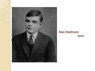
2. Alan Turing was born on June 23, 1912
in Maida Vale, London, England.
At the age of 13 he became particularly
interested in math and science.
Enrolled at King’s College (University of
Cambridge) in Cambridge, England.
In 1936, he delivered a paper,
“Computable Numbers, with an
Application to the
Entscheidungsprobllem”
3. “Automatic Machines”
Turing begins by giving us a
sequence of definitions. The first is
the most famous:
• If at each stage the motion of a
machine is completely determined by
the configuration, we shall call the
machine an “automatic machine” (or a-
machine).
4. For some purposes we might use
machines whose motion is only
partially determined by the
configuration (hence the use of the
word “possible” in x1). When such a
machine reaches one of these
ambiguous configurations, it cannot
go on until some arbitrary choice
has been made by an external
operator.
5. “Computing Machines”
Turing gives us some more
definitions:
If an a-machine prints two kinds of
symbols, of which the first kind
(called figures) consists entirely of
0 and 1 (the others being called
symbols of the second kind), then
the machine will be called a
computing machine.
6. Turing continues:
If the machine is supplied with a
blank tape and set in motion,
starting from
the correct initial m-configuration,
the subsequence of the symbols
printed
by it which are of the first kind will be
called the sequence computed by
the machine.
7. One more small point that
simplifies matters:
The real number whose expression as
a binary decimal is obtained by
prefacing this sequence by a decimal
point is called the number
computed by the machine.
8. A couple more definitions:
At any stage of the motion of the machine,
the number of the scanned square, the
complete sequence of all symbols on the
tape, and the mconfiguration will be said
to describe the complete configuration
at that stage. The changes of the
machine and tape between successive
complete configurations will be called the
moves of the machine.
9. Three points to note:
First, at any stage of the motion of the machine, only a finite of
symbols will have been printed, so it is perfectly legitimate to
speak of “the complete sequence of all symbols on the tape”
even though every real number has an infinite number of
numerals after the decimal point.
Second, the sequence of all symbols on the tape probably
includes all occurrences of [ that do not occur after the last
non-blank square (that is, that do occur before the last non-
blank square); otherwise, there would be no way to
distinguish the sequence h0;0;1; [;0i from the sequence h[;0;
[;0; [;1;0i.
Third, we now have three notions called ‘configurations’; let’s
summarize them for convenience:
1. m-configuration = line number, qn, of a program for a
Turing machine.
2. configuration = the pair: hqn;S(r)i, where S(r) is the symbol
on the currently scanned square, r.
3. complete configuration = the triple: hr, the sequence of all
symbols on the tape,18 qni.
10. “Circular and Circle-Free
Machines”
If a computing machine never
writes down more than a finite
number of symbols of the first kind,
it will be called circular. Otherwise
it is said to be circle-free.
11. Is that what Turing has in mind?
Let’s see. The next paragraph
says:
A machine will be circular if it reaches
a configuration from which there is
no possible move or if it goes on
moving, and possibly printing
symbols of the second kind, but
cannot print any more symbols of
the first kind. The significance of the
12. The first sentence is rather long; let’s
take it phrase by phrase: “A machine
will be circular”—that is, will print out
only a finite number of figures—
[Case 1] it reaches a configuration from
which there is no possible move.” That is,
it will be circular if reaches a line number
qn and a currently scanned symbol S(r)
from which there is no possible move.
How could that be? Easy: if there’s no
line of the program of the form: “Line qn:
If currently scanned symbol = S(r) then. . .
. In that case, the machine because
there’s no instruction telling it to do
anything.
13. But Turing goes on: A machine will
also be circular
[Case 2] it goes on moving, and
possibly printing [only] symbols of
the second kind” but not printing any
more “figures”. Here, the crucial
point is that the machine does not
halt but goes on moving. It might or
might not print anything, but, if it
does, it only prints secondary
symbols.
14. “Computable Sequences and
Numbers”
- A sequence is said to be computable if
it can be computed by a circle-free
machine.
- A number is computable if it differs by
an integer from the number computed
by a circle-free machine.
15. “Examples of Computing Machines”
We are now ready to look at some
“real” Turing machines, more
precisely, “computing machines”,
which, recall, are “automatic” a-
machines that print only figures (‘0’,
‘1’) and maybe symbols of the
second kind. Hence, they compute
real numbers. Turing gives us two
examples, which we will look at in
16. Example I
A machine can be constructed to
compute the sequence 010101. . . .(p.
233.)
Actually, as we will see, it prints
17. The machine is to have the four m-
configurations “b”, “c”, “f”, “e” and is capable
of printing “0” and “1”. (p. 233.)
The four line numbers are (in more legible
italic font): b, c, f , e.
The behaviour of the machine is described in
the following table in which “R” means “the
machine moves so that it scans the square
immediately on the right of the one it was
scanning previously”. Similarly for “L”. “E”
means “the scanned symbol is erased” and
“P” stands for “prints”. (p. 233.)
18.
19. This table (and all succeeding
tables of the same kind) is to be
understood to mean that for a
configuration described in the first
two columns the operations in the
third column are carried out
successively, and the machine then
goes over into the m-configuration
described in the last column. (p.
233, my boldface.)
20. The configuration is the condition,
and the behavior is the action.
A further qualification:
When the second column [that is, the
symbol column] is left blank, it is
understood that the behaviour of the
third and fourth columns applies for any
symbol and for no symbol. (p. 233.)
25. Section 4 “Abbreviated
Tables”
In this section, Turing introduces
some concepts that are central to
programming and software
engineering.
There are certain types of process used
by nearly all machines, and these, in some
machines, are used in many connections.
These processes include copying down
sequences of symbols, comparing
sequences, erasing all symbols of a given
form, etc.
26. In other words, certain sequences of
instructions occur repeatedly in different
programs and can be thought of as being
single “processes”: copying, comparing,
erasing, etc.
Turing continues:
Where such processes are
concerned we can abbreviate the
tables for the m-configurations
considerably by the use of “skeleton
tables”. (p. 235.)
27. There is one small complication: Each
time that this named abbreviation is
needed, it might require that parts of it
refer to squares or symbols on the tape
that will vary depending on the current
configuration, so the one occurrence of
this named sequence in the program
might need to have variables in it:
In skeleton tables there appear capital
German letters and small Greek letters.
These are of the nature of “variables”. By
replacing each capital German letter
throughout by an m-configuration and each
small Greek letter by a symbol, we obtain
the table for an m-configuration.a
28. Of course, whether one uses capital
German letters, small Greek letters, or
something more legible or easier to
type is an unimportant,
implementation detail. The important
point is this:
The skeleton tables are to be
regarded as nothing but
abbreviations: they are not essential.
(p. 236.)