Progresivos

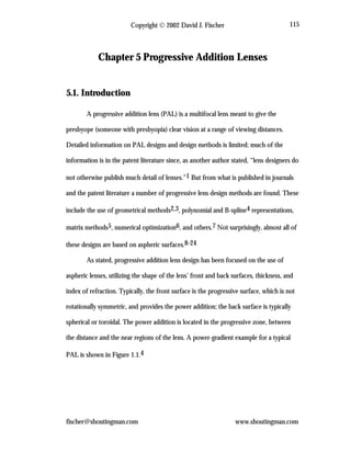
Copyright  2002 David J. Fischer
fischer@shoutingman.com www.shoutingman.com
115
Chapter 5 Progressive Addition Lenses
5.1. Introduction
A progressive addition lens (PAL) is a multifocal lens meant to give the
presbyope (someone with presbyopia) clear vision at a range of viewing distances.
Detailed information on PAL designs and design methods is limited; much of the
information is in the patent literature since, as another author stated, “lens designers do
not otherwise publish much detail of lenses.”1 But from what is published in journals
and the patent literature a number of progressive lens design methods are found. These
include the use of geometrical methods2,3, polynomial and B-spline4 representations,
matrix methods5, numerical optimization6, and others.7 Not surprisingly, almost all of
these designs are based on aspheric surfaces.8-24
As stated, progressive addition lens design has been focused on the use of
aspheric lenses, utilizing the shape of the lens’ front and back surfaces, thickness, and
index of refraction. Typically, the front surface is the progressive surface, which is not
rotationally symmetric, and provides the power addition; the back surface is typically
spherical or toroidal. The power addition is located in the progressive zone, between
the distance and the near regions of the lens. A power-gradient example for a typical
PAL is shown in Figure 1.1.4

116
MainMeridian
φA (dpt)
y>0
y<0
0 21
0
Far Region
(Distance Viewing)
Near Region
(Reading)
Transition Region
}
}
}
Figure 5.1. Example power progression along vertical axis of PAL
In this research, the design of progressive addition lenses via a gradient-index
of refraction is examined. There have been minimal studies of gradient-index
progressive lenses25-28, and many use the GRIN for a constant-power region with the
power progressive added by aspheric surfaces. As suggested, a PAL has a two-
dimensional, non-radially symmetric power form and so requires a non-radially
symmetric index of refraction.29-31 A method to predict and represent the necessary
index profile for the one-dimensional case (unifocal, CVL, axicon) was described in
Chapter 3. It is now extended to two dimensions. This requires both a prediction
method and a representation system for the two-dimensional case.
Furthermore, the progressive lens should be optimized to achieve the desired
power progression while reducing the aberrations to an acceptable level. The optical
aberrations of foremost concern in the initial design are mean oblique error, oblique
astigmatism, and transverse chromatic aberration.29 It is generally understood that
these aberrations should be less than ½-diopter to be acceptable for most people (as
explained previously in section 2.6.1). The lens errors can be further characterized by

117
the wavefront error of rays propagated through the system.32 Perceived aberrations
due to physiological effects are described by quantities such as the blur index and visual
acuity.29,33,34 In this research, mean oblique error and oblique astigmatism are the
aberrations used for design evaluation.
A method to determine the proper index of refraction is used, based on the
modal fitting system from Chapter 3. This method uses the desired power to directly
compute an initial index profile, which is then expressed in terms of basis functions,
for simulation and optimization.
Before examining the problem of predicting the necessary refractive index
profile, a refractive index model is desired. Polynomials are the typical basis functions
for describing refractive index profiles. They provide function and slope continuity and
are very flexible, useful for a variety of geometries. However, a polynomial requires
high-order terms to represent the (relatively) rapidly changing index in the progressive
region, which can introduce numerical instability. This problem is exacerbated if the
polynomial is used to represent the index over the entire lens aperture. In this case it
must represent both a fairly constant index for the distance region and the rapidly
changing index of the progressive region. Another problem with polynomial
representation is that modifying any coefficient affects all of the other coefficients,
because the basis functions are not orthogonal. Thus, the entire lens’ performance is
impacted. This can make it a temperamental system for optimizing the index form and
further complicate full-aperture index design.

118
Cubic Bezier Splines provide the flexibility of polynomials, while not requiring
high-order terms. They also provide localized coefficient effects. However, they do not
readily provide slope or curvature continuity.
Cubic B-splines provide the benefits of polynomials and Bezier Splines,
without the limitations.35-37 They are usually based on low-order polynomials, not
requiring high order terms. They provide continuity of the function, and first- and
second-derivatives. Any coefficient only affects a distinct and limited region of the
function; changing an index coefficient does not affect the entire index profile. Because
any given portion of the B-spline is affected by only a few parameters it is a more
robust method to represent the index over the entire aperture than polynomials. The
weakness of B-splines is their relative complexity compared to polynomials. In this
research B-splines are primarily used for index representation, but polynomials are also
used when particularly convenient.
5.2. Physical Model Description
To properly characterize a PAL, its performance must be evaluated over the
entire lens surface; or more accurately, for the entire range of gaze angles for which the
lens is designed. This requires 2D ray-tracing; the 1D ray-tracing geometry for radially-
symmetric lenses described in Chapter 2 is extended for two dimensions. The ray-
tracing configuration used is that of a “classical astigmometer.”32 The ray-tracing
procedure and lens simulation, including aberration calculations, proceed as described
in Chapter 2.

119
The geometry used is illustrated in Figure 5.2.32 As with the 1D geometry, the
eye’s center of rotation is at Q’, a distance of q’ from the back surface, with the pupil at
p’ along the gaze angle. The lens thickness is t, and has a base index of refraction nO. In
addition to the vertical gaze angle α there is the horizontal gaze angle β, measured
between the optical axis and the projection of the optical ray onto the x-z plane. An
arbitrary ray passing through Q’ can be described by gaze angles α and β. The course
of the power variation is along the vertical axis, called the “Main Meridian.”
Q'
Y
X
Z
q'
p'
Lens
Object
Point
=>
MainMeridian
no
t
Figure 5.2. Schema for ray-tracing 2D ophthalmic lenses.
There is an important aspect of the ray-tracing geometry of which is not
obvious from the one-dimensional case covered in Chapter 1. The coordinate system
of these rays rotates as the gaze angle traverse about the lens—the tangential ray falls
on a transformed vertical axis defined by the line containing the lens vertex and the ray
intersection with the lens’ back surface. So, for a gaze that intersects the vertical axis,
the tangential ray is offset vertically and the sagittal ray offset horizontally. And for a

120
ray which intersects the horizontal axis, the tangential ray is offset horizontally and the
sagittal ray offset vertically in the lens’ coordinate system. This is illustrated in Figure
5.3. Note that when performing ray-tracing simulations the tangential and sagittal rays
are infinitesimally distanced from the ray; their distances are exaggerated in the figure.
Y
Z
X
Lens
Sagittal RayRay
Tangential Ray
Y
X
X'
Y'
X'
Y'
Figure 5.3. Geometry for ray-tracing tangential and sagittal rays. Separation of
the tangential and sagittal rays from the chief ray is exaggerated; they are
actually infinitesimally distanced from the ray.

121
5.3. Index Prediction and Representation Methods
In Chapters 3 and 4 a one-dimensional fitting method was used to describe the
refractive index required for radially symmetric optics. The one-dimensional case is
now extended to the two-dimensional case. Recalling eq. (3.11),
( )
( )2
2T
d n r
r t
dr
φ = − , (3.11)
it is assumed valid and separable over the entire aperture,
( )
( )
2
2
2
2
,
and
,
.
x
y
d n x y
t
dx
d n x y
t
dy
φ
φ
= −
= −
(5.1)
By evaluating over all points (xI, yj) within the fit area, the least-squares fit method is
expressed as ( )n r n F= ⋅
!!
. This is the 2D extension of the 1D method described in
Chapter 3, specifically eq. (3.21). For this research both polynomials and cubic B-
splines are used.
There are two related methods to generate and represent the two-dimensional
refractive index. First, using eq. (5.1) (c.f. eq. (3.14)) and the desired power profile, an
estimate of the index can be analytically computed,
( ) ( )
( ) ( )
( ) ( ) ( )
φ
φ
′ ′ ′= −
′ ′ ′= −
= +
∫∫
∫∫
2
0
2
0
1
, , ,
1
, , , and
, , , .
x
x x
y
y y
x y
n x y x y dx
t
n x y x y dy
t
n x y n x y n x y
(5.2)

122
The power along the y-axis (the Main Meridian) has been described in Chapter
3. But whereas those lenses were radially symmetric, in general progressive addition
lenses are not; the x-axis power must be re-examined.
To achieve the desired effective power, both the tangential and sagittal power
must follow the power progression along the main meridian. As with the tangential
refractive index, a complementary refractive index profile must also be determined for
the sagittal power. Fortunately, an initial estimation is easily achieved using the index
prediction methods and by mimicking the geometric methods used in some aspheric
PAL designs2-4. As explained in Chapter 1, the two primary optical aberrations are
oblique astigmatism and mean optical error. These are eliminated if the sagittal and
tangential powers are identical and equal to the desired power. So for any given y-
position, the sagittal power along the x-direction should be equal to the tangential
power at x=0. From eq. (5.2), the refractive index for the x-axis is calculated as,
( ) ( )21
,
2
x yn x y x y
t
φ= − . (5.3)
The index function can then be fit to e.g. a B-spline function for simulation and
optimization of the lens’ performance. The sagittal power eq. (3.3) is not used here,
because that was for a radially symmetric lens, whereas a PAL is not symmetric.
5.4. Two-Dimensional Refractive Index Representation
5.4.1. Least-Squares Fit Method
Recalling eq. (3.28), the equation for weighting coefficients for a 1D index fit,

123
( )
−
=
!! 1T T
c F F F S , (3.28)
a two-dimensional fit can be computed in the same manner. The matrix F is the basis
functions F(x,y) evaluated at all sampled points, and the vector
!
S is the function being
fit evaluated at all sampled points.
If the basis functions are separable, such that
( ) ( ) ( ),F x y G x H y= , (5.4)
and the function to be fit is sampled on a grid of x,y coordinates, then the fit can be
computed more efficiently using the separated form of eq. (3.28),
( )
( )
1
1
and
.
T T
T T T
d A A A S
c B B B d
−
−
=
=
(5.5)
Here A is the matrix of G(x) evaluated at all sampled x positions, B is the matrix of
H(y) evaluated at all sampled y positions, S is the matrix of functions values for all x, y
positions, and c is the resultant matrix of weighting coefficients.
5.4.2. Overview of Polynomials
A two-dimensional polynomial basis function is expressed as
( ), , l m
l mF x y x y= , (5.6)
and an arbitrary function written as
( ) ( ), ,
0 0
, ,
M L
l m l m
m l
f x y c F x y
= =
= ∑∑ , (5.7)

124
where the coefficients cl,m are the weighting coefficients, computed by e.g. the fit
method in eq. (5.5).
5.4.3. Overview of 1D B-splines
A Spline is an interpolating polynomial; the name coming from a draftsman’s
device, of similar purpose of the French curve, since a Spline originally was a flexible
strip which could be weighted so that, according to the laws of beam flexure, would
pass through several points.35 Splines are a mathematical adaptation of that concept.
Using cubic Splines requires a set of cubic functions to interpolate (data) points which
have been broken up into segments, or patches. Each patch requires its own
interpolating cubic.
B-splines are a specific implementation of cubic Splines. Their name comes
from their bell-like shape; they are Bell-Splines, or B-splines. As interpolating
functions, they are overlapping Gaussian-like functions, individually weighted. Four B-
splines are shown in Figure 5.4.
1 2 3 4 5 6 7
0.1
0.2
0.3
0.4
0.5
0.6
0
0
Figure 5.4. Four Cubic B-splines.

125
Though B-splines are nominally bell-shaped curves, they are easier to use if expressed
differently. Examining the region where the four curves overlap—a region one-quarter
the length of a bell-curve—four unique curves are seen, as in Figure 5.5.
0.2 0.4 0.6 0.8 1
0.1
0.2
0.3
0.4
0.5
0.6
b
1
(u)
b
2
(u)
b
4
(u)
b
3
(u)
0
0
Figure 5.5. Cubic B-spline basis functions.
These curves are the B-spline basis functions. They are cubic polynomials,
( ) ( )
( ) ( )
( ) ( )
( ) ( )
[ ]
= −
= − +
= + + −
=
=
3
1
2 3
2
2 3
3
3
4
1 1 ,6
1 4 6 3 ,6
1 1 3 3 3 , and6
1 , where6
0,1 .
b u u
b u u u
b u u u u
b u u
u
(5.8)
Their second derivatives are
( )
( )
( )
( )
[ ]
′′ = −
′′ = − +
′′ = −
′′ =
=
1
2
3
4
1 ,
2 3 ,
1 3 , and
, where
0,1 .
b u u
b u u
b u u
b u u
u
(5.9)

126
The region they span is a “patch.” The basis functions are normalized (adding them
gives unity), and are independent. To help link these basis functions visually to the
original B-splines, it is helpful to observe that these functions can be "re-assembled" to
get the bell curve, shown in Figure 5.6.
2 3 4 5
0.1
0
1
0.2
0.3
0.4
0.5
0.6
b1(u)
b2(u)
b4(u)
b3(u)
Figure 5.6. Bell curve made of B-spline basis functions, placed sequentially.
Within the patch, the basis functions can be added and weighted to exactly produce any
1D cubic function.
The basis functions are specified with a parametric variable u which spans a
unity distance over a patch region. By weighting the four curves and adding them, a
cubic function can be made; the function within a single patch is
( ) ( )
=
=
−
= ≤ ≤
−
∑
4
1
,
where and .
j j
j
o
o f
f o
s u c b u
x x
u x x x
x x
(5.10)
If a non-unity patch size is desired, u can be scaled for an arbitrary patch size according
to the scaling in eq. (5.10).

127
Consider the earlier example, Figure 5.4. Though there are four B-splines,
spanning seven patches, only one patch contains the four, independent, basis functions.
To use a patch, it must contain all four basis functions. For all seven patches to be
used, an additional three partial B-splines are added at each end to cover the boundary
regions. This is the method used for boundaries in this research, illustrated below.
2 4 6
0.1
0.2
0.3
0.4
0.5
0.6
0
0
1 3 5 7
c
-2
c
-1
c
0
c
1
c
2
c
3
c
4
c
5
c
6
c
7
Figure 5.7. All B-splines required for multi-patch region.
In Figure 5.8, the three center patches are explicitly delineated. Though each
patch contains the four basis functions, each patch has only one independent weighting
coefficient. For example, in the (2,3) patch the c2 weighting coefficient for basis
function b3(u) is the b2(u) coefficient in the adjacent patch (to the right); and is the b1(u)
coefficient in the next adjacent patch. This inter-dependence insures second derivative
continuity for a cubic B-spline function.

128
3 4 5
0.1
0
0.2
0.3
0.4
0.5
0.6
0.7
2
c
0
c
1
c
1
c
2
c
2
c
2
c
3
c
3
c
3
c
4
c
4
c
5
Figure 5.8. One independent coefficient in each patch.
Using eq. (5.10) and the inter-dependence relationships of the weighting
coefficients, a general expression for a B-spline spanning an arbitrary number of
patches can be written. Using L patches over a region ≤ ≤o fx x x , the multiple patch
equation for the B-spline function is
( ) ( )− +
=
= ∑
4
3
1
j l j
j
s u c b u . (5.11)
Equation (5.11) requires
[ ]
−− ∆ −
= ∆ = ≤ <
∆
− 
= ∈ − ∆ 
"
, , ,
, and 0,1, 1 .
f oo
o f
o
x xx l x x
u x x x x
x L
x x
l l L
x
(5.12)
For any L patches, there are L+3 coefficients. Though B-spline patches can be of
varying size in general, they are assumed to be of constant size here.

129
5.4.4. Overview of 2D B-splines
The two-dimensional formulation is an extension of the one-dimensional case.
The 2D bell function is shown in Figure 5.9.
1
2
3
4
5 1
2
3
4
5
0
0.1
0.2
0.3
0.4
Figure 5.9. Two-dimensional bell curve, the basis of 2D B-splines.
The two-dimensional basis functions are
( ) ( ) ( ), ,j k j kb u v b u b v= , (5.13)
where b(u) is given in eq. (5.8). The second derivatives of bjk(u,v) are
( ) ( )
( )
( )
( )
( )
2 2
,
2 2
2 2
,
2 2
,
,
and
,
.
j k j
k
j k k
j
b u v b u
b v
u u
b u v b v
b u
v v
∂ ∂
=
∂ ∂
∂ ∂
=
∂ ∂
(5.14)

130
There are 16 basis functions for the 2D case, written following the example of eq.
(5.11). Given L and M patches along the x-axis and y-axis, respectively, there are
(L+3)*(M+3) control points, with the 2D B-spline written as
( ) ( ) ( )− + − +
= =
= ∑∑
4 4
3 , 3
1 1
, j l k m j k
j k
s u v c b u b v . (5.15)
In addition to the definitions in eq. (5.12), the following definitions for the v variable
are made,
[ ]
−− ∆ −
= ∆ = ≤ <
∆
 −
= ∈ − ∆ 
"
, , ,
, and 0,1, 1 .
f oo
o f
o
y yy m y y
v y y y y
y M
y y
m m M
y
(5.16)
The second derivatives in eq. (5.14) are then given by
( ) ( )
( )
( )
( )
( )
− + − +
= =
− + − +
= =
=
=
∑∑
∑∑
22 4 4
4 , 42 2
1 1
2 24 4
4 , 42 2
1 1
,
and
,
.
j
j l k m k
j k
k
j l k m i
j k
d b ud s u v
c b v
du du
d s u v d b v
c b u
dv du
(5.17)
To fit a 2D B-spline function to a data set, an expression for the “re-
assembled” bell curve in Figure 5.6 is used:
( )
( )
( )
( )
( )
κ
κ κ
κ κ ξ
ξ κ
κ κ ξ
κ κ
κ
>
 − ≤ <

− ≤ <
= =
− ≤ < ∆
 − ≤ <

<
1
2
3
4
0 4
3 3 4
2 2 3
b where
1 1 2
0 0 1
0 0
b
b
b
b
, (5.18)

131
where the ξ variable is a place-holder for either x or y. Using fit data composed of
Nx*Ny points evenly spaced over ≤ ≤o fx x x and ≤ ≤o fy y y , the fitting matrices
are calculated by
( ) ( )( )= − − − ∆
−
∆ = ≤ <
−
b 1
where and 0
1
i o
f o
x
x
A x x x i x
x x
x i N
N
(5.19)
and
( ) ( )( )= − − − ∆
−
∆ = ≤ <
−
b 1
where and 0 .
1
i o
f o
y
y
B y y y j y
y y
y j N
N
(5.20)
Since this is a separable function, the fitting method of eq. (5.5) can be used. The
weighting coefficients of the B-spline equation in eq. (5.15) are provided by the
relationship,
[ ]− + − + = − + − +3 , 3 3 , 3j l k mc c j l k m . (5.21)
5.4.5. Example 1: Small Gaze Angles
Radially symmetric progressive power forms were seen in Chapter 3 and
Chapter 4; here, an equation inspired by US Patent 5,042,9369 is used for the tangential
power along the lens’ main meridian,
( ) ( )
1 s
A
T y y
y
e
κ
φ
φ −
=
+
. (5.22)

132
An example is shown in Figure 5.10, using the values of φA equal to 1 diopter (dpt), κ
equal to 0.60 mm-1
, yS equal to -5 mm, and a 16 mm semi-aperture for a gaze-angle
range of ±30° along the main-meridian.
1.0
0.8
0.6
0.4
0.2
0.0
PowerAddition(dpt)
-30 -20 -10 0 10 20 30
Gaze Angle α (deg)
Figure 5.10. Example power progression from eq. (5.22). The parameter values
are: φA = 1 dpt, κ = 0.60 mm-1
, yS = -5 mm.
According to eq. (5.2), the index of refraction along the main meridian is
( ) ( )
( )2
22
1 2
2
y ys
T o An y n y Li e
t
κ
φ
κ
− 
= − − −  
, (5.23)
where the polylogarithm function Lin(z) is defined as
( )
1
k n
n
k
Li z z k
∞
=
= ∑ . (5.24)
Assuming typical values for the lens geometry of Q equal to 27 mm, and t equal to 3
mm, the predicted refractive index profile is shown in Figure 5.11.

133
-0.020
-0.015
-0.010
-0.005
0.000
∆n
-30 -20 -10 0 10 20 30
Gaze Angle α (deg)
Figure 5.11. Predicted refractive index profile for power progression of Figure
5.10, using the parameter values: Q = 27, t = 3mm.
Ignoring the sagittal power for the moment, an axially symmetric (about the y-
axis) 2D power profile using this power form is used. The refractive index, assuming a
base index of nO equal to 1.5, is fit to 2D B-splines using eq. (5.15) and eq. (5.5) with fit
parameters of: L and M equal 15, xo and yo equal -16 mm, and xf and yf equal +16 mm.
The error of the fit shown in Figure 5.12. The error is largest for α values less than 0,
corresponding to the lower half of the lens, along the main meridian, in the progressive
power region. This is where the index changes the most rapidly (as seen in Figure 5.11),
and thus the fit will be the least accurate. The apparent oscillatory form of the error is
because the B-spline is fundamentally a sequence of cubic polynomial. It will thus
oscillate about the desired curve when the error is minimized but not wholly removed.
This behavior is seen throughout the examples that follow.

134
-200x10
-9
-100
0
100
200
MaximumFitError
-30 -20 -10 0 10 20 30
Gaze Angle α (deg)
Figure 5.12. Error from B-spline fit of laterally-symmetric refractive index
profile. Fit parameters are: L and M = 15, xo and yo = -16 mm, xf and yf =
+16 mm.
To continue with lens simulations, the base lens must first be defined. In
Chapter 2, the ophthalmic lens designs are examined where the aberration control,
optical power, or both, is provided by a GRIN profile.. These designs are compared
with equivalent designs based on both spherical and aspherical homogeneous lenses. In
contrast, here a nominal base lens power in chosen, which is indicative of practical
cases and also provides a convenient design form. The GRIN profile is not used to
provide a constant optical power, nor aberration control for such a lens. Rather, the
GRIN profile is to provide the power progression—a task substantially different from
the purpose of the first design chapter. For the two design examples considered, a one
diopter, spherical lens with minimal mean oblique error (power error) and mean
oblique astigmatism (astigmatism) is used. The base index nO is 1.5, the thickness t is 3
mm, the center of rotation q’ is at 27 mm and the stop p’ is located at 14 mm. The lens’
radii of curvature, computed following the examples of Chapter 1, are 73.32 mm for
the first surface (R1) and 84.56 mm for the back surface (R2). Since this lens description

135
is used in various examples, it is illustrated with a 30 mm semi-aperture, or a 50° gaze
angle. The simulated lens performance is shown in Figure 5.13 and Figure 5.14.
2.0
1.5
1.0
0.5
0.0
Power(dpt)
-40 -20 0 20 40
Gaze Angle α (deg)
Desired Power
Tangential Power
Sagittal Power
Figure 5.13. Performance of base 1 dpt homogeneous, spherical lens. The lens
parameters are: nO = 1.5, t = 3 mm, q’ = 27 mm, p’ = 14 mm, R1 = 73.32
mm, and R2 = 84.56 mm.
-0.30
-0.20
-0.10
0.00
Power(dpt)
-40 -20 0 20 40
Gaze Angle α (deg)
Mean Oblique Error
Oblique Astigmatism
Figure 5.14. The primary aberrations of the one diopter base lens.
The one diopter lens is given the refractive index profile designed for a one
diopter (tangential) power addition, and the lens simulated in same geometry as the
initial lens. The tangential power along the main meridian follows the desired power
until about the 20° gaze angle, where it begins to significantly roll off. This is not

136
surprising; the same behavior was seen in Chapter 3 with concentric varifocal lenses.
This can be corrected by modifying the index design iteratively. Because the current
index profile has no lateral variation, the sagittal power is constant along the main
meridian (except for roll-off effects).
2.0
1.6
1.2
0.8
Power(dpt)
-30 -20 -10 0 10 20 30
Gaze Angle α (deg)
Desired Power
Tangential Power
Sagittal Power
Figure 5.15. Simulated lens performance along main meridian. Note power roll-
off for tangential power near 20° gaze angle.
The difference between the desired power and the tangential power is
computed, and fit to a polynomial (eighth order in this particular case). That equation
for the power difference is integrated, per eq. (5.2), to estimate the refractive index
error. The new refractive index estimate along the main meridian is the previous
estimate plus one-half of the computed error. (Only one-half of the error amount is
used to compensate for the still-present roll-off effects and prevent the iteration from
becoming numerically unstable.) The result of the first iteration is shown in Figure
5.16. After eight iterations, the tangential power follows the desired power curve
closely, as shown in Figure 5.17. Another benefit to the iterative process is that the
resultant refractive index profile is still represented analytically.

137
2.0
1.6
1.2
0.8
Power(dpt)
-30 -20 -10 0 10 20 30
Gaze Angle α (deg)
Desired Power
Tangential Power
Sagittal Power
Figure 5.16. Ray-trace results after first iteration, correcting the tangential power
roll-off.
2.0
1.6
1.2
0.8
Power(dpt)
-30 -20 -10 0 10 20 30
Gaze Angle α (deg)
Desired Power
Tangential Power
Sagittal Power
Figure 5.17. Eight iterations, and tangential power follows desired power.
The lens behavior is seen to be even more complex when the full lens aperture
is examined, as shown in Figure 5.18 and Figure 5.19. The figures are contour plots of
the optical power, within the plane of the lens’ coordinate system. (Refer to Figure 5.2
for details on the lens geometry.) The vertical axis of the plots is the α axis, for vertical
gaze angles, and the horizontal axis is the β axis, for horizontal gaze angles. The upper
half of each contour plot corresponds to the upper half of the lens, where the power is
mostly constant. The lower half corresponds to the lower half of the lens, where the

138
power progressive is located. The curves are isoclines of power in diopters. The
perimeter which encompasses the contour lines and is within the frame of the plot
indicates the usable aperture of the lens. Outside of that boundary, rays do not pass
through the lens, but are lost due to total internal reflection.
Of particular interest in these contour plots is that the sagittal power varies as
the gaze angle moves away from the vertical axis. This variation, despite the lack of
horizontal variation in the refractive index is related to the ray-tracing geometry
described previously (see Figure 5.3). The sagittal ray is not displaced solely from the
horizontal of the gaze ray. Rather, it is along a diagonal relative to the index profile.
This behavior can be predicted, as explained next.
-30
-20
-10
0
10
20
30
GazeAngleα(deg)
-30 -20 -10 0 10 20 30
Gaze Angle β (deg)
1.6
1.4
1.2
1.21
Figure 5.18. Contour plot of tangential power from lens simulation. Labeled
curves are optical power isoclines in diopters.

139
-30
-20
-10
0
10
20
30
GazeAngleα(deg)
-30 -20 -10 0 10 20 30
Gaze Angle β (deg)
1.61.6
1.41.4
1.21.2
11
Figure 5.19. Contour plot of sagittal power from lens simulation. Note
increasing power away from main meridian.
5.4.6. Refractive Index Coordinate Transform
Ophthalmic lens literature often uses plots of surface power to aid in the
assessment of spherical and aspherical lens performance and quality. An analogous
approach can be taken with GRIN PALs by estimating lens performance from the
index of refraction. The approach is to calculate the tangential and sagittal power of the
lens according to the refractive index only, without consideration to surface shape or
ray-tracing simulations. And this can be extended to estimate the mean power and
astigmatism.
As explained by Figure 5.3 ray-tracing requires a rotated coordinate system
according to the gaze-angle. Though a lens’ behavior could be estimated using eq. (5.1),

140
this does not account for the rotated coordinate system of the tangential and sagittal
rays. To improve the estimate, the transform is applied to the position variables. In the
case of B-splines, the second-derivatives given by eqs. (5.9) and (5.17) are used.
Thus, to compute the optical powers in the ray-trace geometry, derivatives of
the fitting function are needed along the sagittal and tangential axes. The index
derivatives are aligned with the tangential and sagittal axes by a coordinate transform,
shown in Figure 5.20. The transform point is placed along the new y’ axis and
substituted back into the coordinate-transform equations, yielding the new coordinate
system variables in terms of the non-transformed x,y coordinates, given in eq. (5.25).
y
y
x
x
(x,y)
(0,y)
θ
Figure 5.20. Geometry for tan/sag coordinate transform.
( ) ( ) ( )
( )θ
′ ′ ′= = +
=
2 2
, 0, 0, ,
tan .
x y y x y
x y
(5.25)
The 2D basis functions of (5.13) are expanded in terms of x and y, using the
expressions in eq. (5.12) for the u and v variables. The basis functions are differentiated
with respect to x and y and eq. (5.25) substituted. This leads to 16 equations for both
the tangential and sagittal indicial derivatives. These equations are given in Appendix B,
eqs. (B.2)-(B.33).

141
Using these equations, the predicted behavior of the current PAL is shown in
Figure 5.21 and Figure 5.22. These contour plots depict the same geometry as the
previous two plots: they show the lines of constant optical power within the lens’
coordinate system. Comparing the graphs in Figure 5.21 and Figure 5.22 to Figure 5.18
and Figure 5.19 the “indicial” estimation qualitatively predicts the lens’ performance.
However, the roll-off effect is not estimated. Thus, the sagittal power variation away
from the main meridian is due to the gaze-angle geometry, despite the lack of
horizontal variation in the refractive index profile.
-30
-20
-10
0
10
20
30
GazeAngleα(deg)
-30 -20 -10 0 10 20 30
Gaze Angle β (deg)
1.8
1.6
1.41.2
11
Figure 5.21. The tangential power addition is estimated using the tangential
coordinate transform and refractive index function. This for the initial
design, ignoring sagittal power concerns.

142
-30
-20
-10
0
10
20
30
GazeAngleα(deg)
-30 -20 -10 0 10 20 30
Gaze Angle β (deg)
1.61.6
1.41.4
1.21.2
1
Figure 5.22. The sagittal power addition is estimated using the sagittal
coordinate transform and refractive index function. This for the initial
design, ignoring sagittal power concerns.
5.4.7. Lateral Variation in Refractive Index Profile
So far, the desired sagittal power has not been addressed. It is accounted for
using eqs. (5.3), (5.22), and (5.23), to derive an initial estimation of the required index
of refraction:
( ) ( )
( )
( )
( )
2
2
22
1 2
,
2 1
y ysA
o A y ys
x
n x y n y Li e
t e
κ
κ
φ
φ
κ
−
−
 
 = − + − −
 +
 
. (5.26)
This expresses the lateral variation in the refractive index needed to provide the sagittal
power along the main meridian. The resultant index profile is shown in Figure 5.23.

143
The maximum fit error along the vertical edge of the refractive index function is shown
in Figure 5.24. Again, the index fit error is greatest in the progressive region.
-30
-15
0
15
30
-30
-15
0
15
30
,n
-0.06
-0.04
-0.02
0.0
(deg)
= (deg)
Figure 5.23. Refractive index profile to provide both the desired tangential
power and the desired sagittal power along the main meridian. This is
achieved by incorporating the necessary lateral variation in the refractive
index profile into to provide the sagittal power. The index function is fit
to 2D B-splines with fit parameters: L and M = 21, xo and yo = -30 mm, xf
and yf = +30 mm.
-10x10
-6
-5
0
5
10
MaximumFitError
-30 -20 -10 0 10 20 30
Gaze Angle α (deg)
Figure 5.24. The largest error from a B-spline fit of the refractive index profile
(shown in Figure 5.23) is along the vertical at the horizontal edge
(coordinates (y,xf)).

144
Using this new refractive index profile, the lens behavior is estimated by the
coordinate-transformed refractive index calculations, shown in Figure 5.25 and Figure
5.26. These contour plots show the same information as the previous contour plots of
ray-traced lens simulation. The important difference is that these optical power values
are predicted from the refractive index, and are not based on ray-tracing simulations.
The tangential power behaves as previously and the sagittal power now increases along
the main meridian as desired. The lens is also ray-traced, shown in Figure 5.27 and
Figure 5.28. It is seen that the behavior predicted by physical simulation is qualitatively
the same as predicted by the coordinate-transformed refractive index functions. This
shows that a progressive GRIN lens can be qualitatively simulated solely on the
refractive index profile, without the need for the more computationally expensive ray-
tracing procedure.
-30
-20
-10
0
10
20
30
-30 -20 -10 0 10 20 30
22 1.8
1.2
11
GazeAngle=(deg)
Gaze Angle (deg)
Figure 5.25. Tangential power is estimated via the coordinate transform.

145
-30
-20
-10
0
10
20
30
GazeAngle=(deg)
-30 -20 -10 0 10 20 30
Gaze Angle (deg)
2.1 2.1
1.9
1.7
1.3 1.3
1.1 1.1
1.1
0.9 0.9
Figure 5.26. Sagittal power is estimated via the coordinate transform.
-30
-20
-10
0
10
20
30
-30 -20 -10 0 10 20 30
2 2
1.8
1.8
1.6 11
1
GazeAngle=(deg)
Gaze Angle (deg)
Figure 5.27. Contour plot of tangential power from ray-traced lens simulation.

146
-30
-20
-10
0
10
20
30
-30 -20 -10 0 10 20 30
2 2
1.8 1.6 1.4
1.21.2
1.2
1
GazeAngle=(deg)
Gaze Angle (deg)
Figure 5.28. Contour plot of sagittal power from lens simulation.
The initial prediction of the two-dimensional refractive index profile is
effective, providing much of the desired behavior. But it suffers from roll-off effects at
higher, off-axis ray angles. This is more easily seen in Figure 5.29, a plot of the optical
power along the main meridian.
The roll-off in the tangential power can be corrected by an iterative process.
The difference between the desired power and the tangential power is converted to a
refractive index error, using eq. (5.2). This refractive index error is fit to a polynomial
(for convenience) and subtracted from the analytical refractive index equation. The new
refractive index is ray-traced and the iteration continued. The corrected tangential
power is shown in Figure 5.30 with the initial sagittal power.

147
2.0
1.6
1.2
0.8
Power(dpt)
-30 -20 -10 0 10 20 30
Gaze Angle α (deg)
Desired Power
Tangential Power
Sagittal Power
Figure 5.29. Lens performance along main meridian, with initial two-
dimensional refractive index design.
2.0
1.6
1.2
0.8
Power(dpt)
-30 -20 -10 0 10 20 30
Gaze Angle α (deg)
Desired Power
Tangential Power
Sagittal Power
Figure 5.30. The tangential power roll-off is corrected by an iterative method.
The sagittal power has not been corrected, and the initial value is shown.

148
2.0
1.6
1.2
0.8
Power(dpt)
-30 -20 -10 0 10 20 30
Gaze Angle α (deg)
Desired Power
Tangential Power
Sagittal Power
Figure 5.31. The corrected tangential power is combined with the sagittal power
rule. This causes the sagittal power to be over-compensated.
2.0
1.6
1.2
0.8
Power(dpt)
-30 -20 -10 0 10 20 30
Gaze Angle α (deg)
Desired Power
Tangential Power
Sagittal Power
Figure 5.32. Sagittal power corrected via 10 iterations, as with the tangential
power.

149
-0.02
0.00
0.02
Power(dpt)
-30 -20 -10 0 10 20 30
Gaze Angle α (deg)
Mean Oblique Error
Oblique Astigmatism
Figure 5.33. Aberrations along main meridian.
The sagittal power is then recomputed, according to eq. (5.3), using the
corrected tangential refractive index. The new sagittal power estimate is shown below,
in Figure 5.31. The sagittal power is then corrected iteratively. The results after 10
iterations are shown in Figure 5.32 and the optical errors are shown in Figure 5.33.
With the new refractive index function, the lens is ray-traced to determine the
performance and the primary aberrations calculated. The results are shown in the
following five plots, Figure 5.34, Figure 5.35, Figure 5.36, Figure 5.37, Figure 5.38.

150
-30
-20
-10
0
10
20
30
-30 -20 -10 0 10 20 30
2
22
1.8
1.8
1.2
1
GazeAngle=(deg)
Gaze Angle (deg)
Figure 5.34. Tangential power after the tan. and sag. powers are corrected.
-30
-20
-10
0
10
20
30
-30 -20 -10 0 10 20 30
2
2
2
1.8
1.6
1.21.2
1
1
GazeAngle=(deg)
Gaze Angle (deg)
Figure 5.35. Sagittal power after the tan. and sag. powers are corrected.

151
-30
-20
-10
0
10
20
30
-30 -20 -10 0 10 20 30
2.0
2.02.0
1.8
1.6
1.2
1.0
1.01.0
1.0
GazeAngle=(deg)
Gaze Angle (deg)
Figure 5.36. Mean-oblique power, after roll-off correction.
This lens simulation shows that the progressive lens has the desired power
progression and acceptable aberrations in the upper distance portion, along the main
meridian, and in the lower near portions. The aberrations are also small in the vicinity
of the main meridian. The errors do increase significantly in the middle, side areas of
the lens. These errors are not addressed in the present work.

152
-30
-20
-10
0
10
20
30
-30 -20 -10 0 10 20 30
0.6
0.6
0.40.4
0.2
0.2
0.2
0.2
0.2
0.0 -0.2-0.2
-0.6 -0.6
GazeAngle=(deg)
Gaze Angle (deg)
Figure 5.37. Mean oblique astigmatism, after roll-off correction.
-30
-20
-10
0
10
20
30
-30 -20 -10 0 10 20 30
0.6 0.6
0.20.2
0.0
0.0
-0.2-0.2
-0.6-0.6
GazeAngle=(deg)
Gaze Angle (deg)
Figure 5.38. Mean power error, after roll-off correction.

153
5.4.8. Example 2: Large Gaze Angles
The design process is now repeated for a lens with larger gaze angles, of ±50°
along the main-meridian. The power form is again eq. (5.22), with φA equal to 3 dpt, κ
equal to 0.25 mm-1
, and yS equal to -10 mm. The power form is shown in Figure 5.39
and the predicted refractive index in Figure 5.40. This index form is currently not
physically realizable by any known GRIN manufacturing technique. But for the present
research, this concern will be set aside, to pursue what could be done if an arbitrary
index of refraction could be fabricated.
3
2
1
0
Power(dpt)
-40 -20 0 20 40
Gaze Angle α (deg)
Figure 5.39. Desired power profile for large gaze-angle lens.

154
-0.3
-0.2
-0.1
0.0
∆n
-40 -20 0 20 40
Gaze Angle α (deg)
Figure 5.40. Predicted refractive index profile for power progression of Figure
5.39 using the parameter values Q = 27, t = 3mm.
The necessary two-dimensional refractive index profile is estimated using eq.
(5.26). It is then fit to a B-spline, for ray-tracing using the fit parameters: L equals 21
and M equals 53, xo and yo equal -33 mm, and xf and yf equal +33 mm. The maximum
fit error is shown in Figure 5.41. As seen in the previous example (Figure 5.12), the fit
error is greatest in the progressive region where the index changes most rapidly. The
lens’ performance is also estimated via the coordinate-transformed refractive index
equations. The expected tangential and sagittal power performance is as desired along
the main meridian and adjacent regions, as seen in Figure 5.42 and Figure 5.43. This
shows that this is a worthwhile refractive index form to investigate, even for the larger
aperture and larger gaze-angles

155
-1.0x10
-6
-0.5
0.0
0.5
1.0
MaximumFitError
-40 -20 0 20 40
Gaze Angle α (deg)
Figure 5.41. B-spline fit error of laterally-symmetric refractive index profile. Fit
parameters are: L = 21 and M = 53, xo and yo = -33 mm, xf and yf = +33
mm.
-50
-40
-30
-20
-10
0
10
20
30
40
50
-40 -20 0 20 40
4
4
3.8
3.8
3.4
3
2
1.6
1.4
1.2
1 1
GazeAngle=(deg)
Gaze Angle (deg)
Figure 5.42. Tangential power estimate based on initial design, computed using
the tangential coordinate transform.

156
-50
-40
-30
-20
-10
0
10
20
30
40
50
-40 -20 0 20 40
3.8
3.83.8
3.4
33
3
2
22
1.6
1.4
1.2
1.2
GazeAngle=(deg)
Gaze Angle (deg)
Figure 5.43. Sagittal power estimate based on initial design, computed using the
sagittal coordinate transform.
-0.15
-0.10
-0.05
0.00
0.05
0.10
Power(dpt)
-40 -20 0 20 40
Gaze Angle α (deg)
Mean Oblique Error
Oblique Astigmatism
Figure 5.44. Performance of 1-dpt base lens with design parameters: nO equal to
1.65, R1 equal to 114.42 mm, k1 equal to 1.40 mm-2
, R2 equal to 146.69 mm,
and k2 equal to -2.50 mm-2
.
A one-diopter base lens is again used, re-designed for better performance at
large gaze-angles. This lens is a bi-asphere with a 33 mm semi-aperture and base index

157
nO equal to 1.65. The first surface has a radii of curvature R1 equal to 114.42 mm and a
conic constant k1 equal to 1.40 mm-2
. The second surface has a radii of curvature R2
equal to 146.69 mm and a conic constant k2 equal to -2.50 mm-2
. The base lens’
performance is shown in Figure 5.44.
Ignoring sagittal power concerns initially, the lateral variation in the index of
refraction is removed and the lens ray-traced. The initial performance is shown in
Figure 5.45. Like the first example, the tangential power follows the desired curve until
about halfway down the main-meridian.
5
4
3
2
1
0
Power(dpt)
-40 -20 0 20 40
Gaze Angle α (deg)
Desired Power
Tangential Power
Sagittal Power
Figure 5.45. Lens performance along main meridian (y-axis) based on initial
PAL design.
The tangential power roll-off is corrected iteratively using a 14th
order
polynomial for fitting to the power error; a 14th
order polynomial was the minimum
order that worked satisfactorily. The final correction factor is a 16th
order polynomial,
because the index function is two orders higher than the power function. The final
coefficients for the correction polynomial are given in Table 5.1. The corrected index
function is ray-traced and the tangential power shown in Figure 5.46.

158
Correction
Term
Coefficient
Value
y 0
y2
0
y3
4.012*10-8
y4
1.274*10-8
y5
2.079*10-10
y6
-4.364*10-11
y7
-2.633*10-12
y8
4.015*10-15
y9
3.861*10-15
y10
2.895*10-17
y11
-3.759*10-18
y12
-4.676*10-20
y13
1.985*10-21
y14
2.992*10-23
y15
-4.370*10-25
y16
-7.223*10-27
Table 5.1. Coefficients for correction polynomial used to remove roll-off in
tangential power along the main meridian.
The predicted refractive index term for the sagittal power is modified according
to the corrected tangential power and incorporated into the refractive index equation.
This provides the desired sagittal power along the majority of the main meridian, as
seen in Figure 5.47.
The sagittal power is then corrected iteratively, also using a 14th
order
polynomial. The resultant lens performance along the main meridian is shown in Figure
5.48 and the correction-term polynomial coefficients are given in Table 5.2. The
resultant refractive index profile for the entire lens is shown in Figure 5.49.

159
5
4
3
2
1
0
Power(dpt)
-40 -20 0 20 40
Gaze Angle α (deg)
Desired Power
Tangential Power
Sagittal Power
Figure 5.46. Tangential power after roll-off correction.
5
4
3
2
1
0
Power(dpt)
-40 -20 0 20 40
Gaze Angle α (deg)
Desired Power
Tangential Power
Sagittal Power
Figure 5.47. Initial design with sagittal power considered.
5
4
3
2
1
0
Power(dpt)
-40 -20 0 20 40
Gaze Angle α (deg)
Desired Power
Tangential Power
Sagittal Power
Figure 5.48. Corrected sagittal power.

160
Correction
Term
Coefficient
x2
y 2.221*10-7
x2
y2
-2.459*10-8
x2
y3
-1.706*10-9
x2
y4
-3.154*10-10
x2
y5
-2.293*10-12
x2
y6
1.975*10-12
x2
y7
6.945*10-14
x2
y8
-3.048*10-15
x2
y9
-1.416*10-16
x2
y10
2.309*10-18
x2
y11
1.238*10-19
x2
y12
-6.588*10-22
x2
y13
-4.055*10-23
x2
y14
-2.447*10-26
Table 5.2. Correction polynomial coefficients for sagittal power.
-50
-25
0
25
50
-50
-25
0
25
50
-0.5
-0.4
-0.3
-0.2
-0.1
0.0
,n
(deg)
= (deg)
Figure 5.49. Refractive index profile after correcting main-meridian power
performance.
The lens is then ray-traced over the entire aperture with the modified refractive
index profile. The tangential power (Figure 5.50) and sagittal power (Figure 5.51) both
behave as desired in the upper, nearly-constant power region and in the progressive

161
region along the main meridian and adjacent regions. The power deviates from the
desired form in the lower, lateral regions.
The mean power (Figure 5.52), mean oblique error (Figure 5.53), and oblique
astigmatism (Figure 5.54) are computed. The mean power, as shown in the power error
plot, has less than ½ dpt error for the majority of the gaze angles, with the error
increasing significantly in the outer regions. The astigmatism also is low in the upper,
constant power region and along the main meridian. It is under ½ dpt for
approximately ±10° along the main meridian. It increases significantly in the lateral
regions.
-50
-40
-30
-20
-10
0
10
20
30
40
50
-40 -20 0 20 40
4.0
4.0
4.0
3.5
3.0
2.0
1.5
1.0 1.0
GazeAngle=(deg)
Gaze Angle (deg)
Figure 5.50. Ray-traced tangential power. The tangential power performance
was corrected for roll-off using an iterative correction method.

162
-50
-40
-30
-20
-10
0
10
20
30
40
50
-40 -20 0 20 40
4.04.0
4.0
3.5
3.0
2.5
1.5
1.0
GazeAngle=(deg)
Gaze Angle (deg)
Figure 5.51. Ray-traced sagittal power, after roll-off correction.
-50
-40
-30
-20
-10
0
10
20
30
40
50
GazeAngle=(deg)
-40 -20 0 20 40
Gaze Angle (deg)
4.0 4.0
3.5
3.0
2.0
1.5
1.01.0
1.0
Figure 5.52. Mean-oblique power.

163
-50
-40
-30
-20
-10
0
10
20
30
40
50
-40 -20 0 20 40
1.0 1.0
0.5 0.5
0.20.2
0.0
-0.2-0.2
-0.5-0.5
GazeAngleα(deg)
Gaze Angle β (deg)
Figure 5.53. Mean power error.
-50
-40
-30
-20
-10
0
10
20
30
40
50
-40 -20 0 20 40
1.0 1.00.5
0.2
0.2
0.2
0.0
0.0
-0.2
-0.5
-0.5
-1.0
-1.0
GazeAngle=(deg)
Gaze Angle (deg)
Figure 5.54. Mean oblique astigmatism.

164
This lens simulation shows that it is possible to design a GRIN PAL for use at
large gaze angles. As with the small gaze-angle example, the distance and near portions
are error free and the performance along the main meridian is excellent. The significant
aberrations are in the mid-lateral regions.
The cause of the optical aberrations is suggested by Figure 5.42 and Figure
5.43; they are made evident in the following figures: Figure 5.55 and Figure 5.56. These
two plots show the second-derivative of the refractive index in the coordinate-
transformed geometry. Since optical power is related to the second-derivative of the
refractive index, regions where the second-derivative changes rapidly can be expected
to have a rapid change in optical power. This explains the source of the aberrations in
the mid-lateral regions. The refractive index second derivative changes rapidly,
particularly so for the sagittal direction (Figure 5.56). Thus, the aberrations shown by
the ray-tracing simulations are anticipated by the curvature of the refractive index.
Correcting these aberrations requires that the gradient-index profile curvature away
from the vertical axis be made to follow the same form as that along the main
meridian.

165
-50
-25
0
25
50
-50
-25
0
25
50
-0.004
-0.002
0
0.002
(deg)
= (deg)
Figure 5.55. The tangential second-derivative of the refractive index, calculated
using the coordinate-transform equations. The curvature of the refractive
index away from the vertical axis (α) follows a different form than near it.
This is the cause of the worst aberrations in the mid-lateral regions.
-0.002
-0.001
0
0.001
-0.002
-0.001
0
-50
-25
0
25
50
-50
-25
0
25
50
(deg)
= (deg)
Figure 5.56. The sagittal second-derivative of the refractive index, calculated
using coordinate-transform equations. The curvature of the refractive
index changes rapidly in the lateral. This is the cause of the worst
aberrations in the mid-lateral regions.

166
5.4.9. Optimizing B-spline Index of Refraction
At this point, it might seem prudent to numerically optimize the index of
refraction to improve the lens’ performance. This was investigated using the well-
known maximum-descent algorithm.38 The optimizing program used the ray-tracing
program to compute a merit function based on the aberrations of the lens within the
area being manipulated. The optimizer then began at the top of the lens, along the
main meridian, in what is the mostly homogenous region of these designs. Within the
first patch the free control points of the B-spline (representing the refractive index)
were modified to improve the lens performance. The merit function was based on ray-
trace results within both the manipulated patch and a user-specified number of
adjacent patches. This was to help prevent the optimization from wholly sacrificing
performance further along the main meridian while working on the present region.
When the optimizer had improved the current region as much as possible,
within the constraints of the maximum-descent method, it stepped one patch further
along the main meridian and repeated the process. This continued until the optimizer
traversed the main meridian. If the optimizer was to work on the entire lens, after
traversing the vertical axis, it repeated the process along the vertical but stepped one
patch to the side.
This simple optimization technique was quite useful for one-dimensional cases
(along the main meridian only); it could replace the iterative correction technique.
However, optimizing the whole of the lens posed significant challenges. Specifically, as
each patch was modified it further affected the lens’ performance subsequent to it;

167
generally negatively. Effectively, the aberrations were pushed into the lower lateral
regions, as the lens was optimized. Eventually, the optimizer was no longer be able
overcome the aberrations were “pushed” into the region.
The optimization of gradient index profiles represented by two-dimensional B-
splines shows promise. But the optimization problems are not yet overcome, and
further investigation of appropriate optimization methods are left to future research.
5.5. Conclusion
The first systematic approach to designing a gradient-index profile for
progressive addition lenses has been given. This brings several new tools to GRIN lens
design, until now used for the design of constant power, rotationally symmetric lenses.
First, these designs call for substantially larger apertures and greater index changes than
normally considered in GRIN lens designs. Second, tools for the design of non-
symmetric lenses were developed, in contrast to conventional methods for design of
symmetric lenses. Third, a method for predicting the refractive index profile for an
arbitrary power form is explained; likewise distinct from conventional GRIN lens
design.
The design tools demonstrate how to use B-splines for index representation.
This is also novel, compared with the traditional use of polynomials. These functions
promise even greater control over index profile computation and optimization.
Finally, this work provides a potential method for new and exciting GRIN lens
designs. Though the work here addresses progressive addition lenses, it could also be
used for designing contact lenses with arbitrary power forms. Such a lens could

168
conceivably be used for providing exact correction for the eye’s aberration, providing
the wearer perfect vision. Or, perhaps new intra-ocular lenses could be designed, for
those with aphakia. Thus, with these tools, a new area of GRIN lens design is made
available.
5.6. References
1C. Fowler, “Recent trends in progressive power lenses,” Ophthalmic Physiological
Optics 18 (2), 234-7 (1998).
2Bernard Maitenaz, “Variable Power Lenses,” presented at the International
Ophthalmic Optical Congress, London, 1961 (unpublished).
3W. Lenne, “Visual reliability: the conception of Varilux lenses,” SPIE Proceedings
601, 24-30 (1986).
4G. M. Fuerter, “Ophthalmic lens design with splines,” SPIE Proceedings 601, 9-16
(1986).
5J. Alonso, J. A. Gomez-Pedrero, and E. Bemabeu, “Local dioptric power matrix in a
progressive addition lens,” Ophthalmic Physiological Optics 17 (6), 522-9 (1997).
6J. Loos, G. Geiner, and H. P. Seidel, “A variational approach to progressive lens
design,” Computer Aided Design 30 (8), 595-602 (1998).
7G. H. Guilino, “Design philosophy for progressive addition lenses,” Applied Optics
32 (1), 111-17 (1993).
8Jeffrey H. Roffman, Timothy A. Clutterbuck, and Yulin X. Ponte Lewis, US
5,805,260 (Sept. 8 1998).

169
9Gunther Guilino, Herbert Pfeiffer, and Helmut Altheimer, US 5,042,936 (Aug. 27
1991).
10Chun-Shen Lee and Michael J. Simpson, US 5,699,142 (Dec. 16 1997).
11Christian Harsigny, Christian Miege, Jean-Pierre Chauveau et al., US 5,488,442 (Jan.
30 1996).
12Scott W. Smith, US 5,691,798 (Nov. 25 1997).
13A. A. Naujokas, US 3,485,556 (Dec. 23 1969).
14Valdemar Portney, US 5,657,108 (Aug. 12 1997).
15Bernard F. Maitenaz, US 3,910,691 (Oct. 7 1975).
16Bernard F. Maitenaz, US 3,687,528 (Aug. 29 1972).
17Gerhard Kelch, Hans Lahres, Konrad Saur et al., US 5,784,144 (July 21 1998).
18John F. Isenberg, US 5,715,032 (Feb. 3 1998).
19Rudolf Barth, US 5,771,089 (June 23 1998).
20Eric F. Barkan and David H. Sklar, US 4,838,675 (June 13 1989).
21John T. Winthrop, US 4,861,153 (Aug. 29 1989).
22John T. Winthrop, US 5,726,734 (March 10 1998).
23Francoise Ahsbahs and Claude Pedrono, US 5,708,493 (Jan. 13 1998).
24Francoise Ahsbahs, Thierry Baudart, and Gilles Le Saux, US 5,719,658 (Feb. 17
1998).
25Kitani Akira, EP 0,872,755 (Oct. 21 1998).
26R. S. Moore, US 3,718,383 (Feb. 27 1973).

170
27Gunther Guilino, Helmut Altheimer, and Herbert Pfeiffer, US 5,148,205 (Sept. 15
1992).
28J. R. Hensler and Charles H. Rosenbauer, US 3,542,535 (Nov. 24 1970).
29D. A. Atchison, “Spectacle lens design: a review,” Applied Optics 31 (19), 3579-85
(1992).
30Tony Jarratt, “Progressive Lenses,” Optical World (March), 13-16 (2000).
31C. M. Sullivan and C. W. Fowler, “Progressive addition and variable focus lenses: a
review,” Ophthalmic Physiological Optics 8 (4), 402-14 (1988).
32B. Bourdoncle, J. P. Chauveau, and J. L. Mercier, “Traps in displaying optical
performances of a progressive-addition lens,” Applied Optics 31 (19), 3586-93 (1992).
33D. A. Atchison, “Modern optical design assessment and spectacle lenses,” Optica
Acta 32 (5), 607-34 (1985).
34David A. Atchison, “Spectacle Lens Design - Development and Present State,”
Austrailian Journal of Optometry 67 (3), 97-107 (1984).
35Paul Dierckx, Curve and surface fitting with splines (Clarendon, Oxford ; New York,
1993).
36Carl De Boor, A practical guide to splines (Springer-Verlag, New York, 1978).
37P. M. Prenter, Splines and variational methods (Wiley, New York, 1975).
38William H. Press, “Minimzation or Maximization of Functions,” in Numerical recipes in
C : the art of scientific computing (Cambridge University Press, Cambridge, New York,
1992), pp. 395-455.

Progresivos

Recommended

Recommended

More Related Content

What's hot

What's hot (17)

Viewers also liked

Viewers also liked (19)

Similar to Progresivos

Similar to Progresivos (20)

More from Yesenia Castillo Salinas

More from Yesenia Castillo Salinas (20)

Recently uploaded

Recently uploaded (20)

Progresivos