1. MODELING THE JET GEOMETRY
Relativistic jets in AGN are one of the most interesting and complex structures in the Universe. Some of the jets
can be spread over hundreds of kilo parsecs from the central engine and display various bends, knots and
hotspots. Observations of the jets can prove helpful in understanding the emission and particle acceleration
processes from sub-‐arcsec to kilo parsec scales and the role of magnetic field in it.
The M87 jet has many bright knots as well as regions of small and large bends. We attempt to model the jet
geometry using the observed 2-‐dimensional structure. The radio and optical images of the jet show evidence of
presence of helical magnetic field throughout. Using the observed structure in sky frame, our goal is to gain an
insight into the intrinsic 3 dimensional geometry in the jet’s frame. The structure of the bends in jet’s frame may
be quite different than what we see in the sky frame. The knowledge of the intrinsic structure will be helpful in
understandingthe appearance of the magnetic field and hence polarization morphology.
The figures and equations below show the geometry of a bend as well as the observed projection. The equation
set is non-‐linear and has degeneracies. We use Bayesian methods to statistically estimate model parameters for
the jet geometry as shown. (Fig 2 and 3).
227th AAS
Meeting,
Kissimmee,
FL
Optical
and
radio
images
of
the
M87
jet
show
a
huge
variety
of
parsec-‐scale
bends
and
helical
distortion
from
HST-‐1
to
knot
C.
The
sinusoidal
pattern
in
the
outer
jet
is
observed
in
both
bands,
suggesting
a
possible
double
helical
structure.
We
developed
a
mathematical
model
that
converts
the
observed
2D
projection
of
the
jet
to
a
3D
configuration
by
using
three
inputs:
the
viewing
angle
(estimated
from
20
years
of
HST
monitoring
of
the
jet),
distances
and
relative
angles
between
bends
measured
from
the
HST
optical
and
VLA/VLBA
radio
images
of
the
M87
jet.
Our
model
is
written
in
Python,
combining
nonlinear
optimization
methods
and
computer
graphics
to
describe
and
demonstrate
the
jet
geometry.
We
are
extensively
testing
the
scripts
to
compare
stability
of
the
model,
optimization
techniques, and
model
with
the
data
of
galactic
jets,
focusing
on
M87.
THEORY
Parameterized
3D
Model
of
Jet
Geometry
• Points
O,
A,
B
represent
arbitrary
knots
in
the
jet.
• Applying
Pythagorean
theorem
and
trigonometric
identities
in
triangle
ABC
and
its
projections
creates
an
equation
set
describing
model of
local
jet
geometry
containing
5
equations
and
5
unknowns:
𝛼, 𝛽, 𝜙, 𝜉, 𝑑.
• A
parameter
four-‐vector
x
=
( 𝜃,
𝜉,
𝜙,
𝑑)
describes
the
local
bend
structure
• Apparent
bend
angle
𝜂,
and
apparent
bend
length
s
are
measured
from
the
image
of
the
jet.
• Statistically estimating model parameters by Bayesian analysis based on the Markov Chain Monte Carlo
(MCMC) method.
• Five-‐dimensionalparameter space: v = (𝛼, 𝛽, 𝜙, 𝜉, 𝑑)
• A group of initial guesses (walkers) evenly distributedaround the definitiondomain.
• Uniform non-‐informativeprior
• Likelihoodfunctionis derived from the equation set that describes the jet geometry.
• Once instabilities were found in the solutions, using the log-‐likelihood of the equations was performed to
restrict the solutionsto be in the first quadrant.
• Posterior probability distribution (PPD) is normalized, so that the closer to solution vector of the equation
set, the larger the joint posterior probability. So the corresponding parameter vector at maximum A
posteriori (MAP) is the solutionvector of the equation set.
• The resulting corner plot shows 1D marginalized PPDs for all 5 model parameters, and correlations between
each pair of parameters are also shown in the plot.
• Finally, MAP estimation is applied to obtain the parameter vector which describes the local jet structure
best.
• We tried several methods to solve the nonlinear equation set, including MCMC, simulated annealing and
Newton’s method. Of these, MCMCgave the strongest constraints and least instabilities.
Parameter
Estimation
by
MCMC
Description
of
Code
• Maximum Position Code iterates from the nucleus to the end of the jet finding the maximum values of each
column of the image. We compare maximum values using Gaussian weights.
• From finding the maximum values of each column in the image matrix, we determine the position of knots
in the jet.
• From the results of the average and maximum values, the bends in the jet are determined to find the values
of distances and angles between knots in the sky frame. The distances and angles of the jet geometry are
easily found using trigonometry relations between the bends.
Figure
8.
Corner
Plot
of
α,
β, ɸ,
ξ,
and
d
from
the
modeling
result
when
use
η
=
24.37°,
s
=
85.67
pc,
and
θ =
15° as
input,
where
η and
s
are
from
the
testing
result.
The
solution
vector
at
MAP
is
(α,
β,
ɸ,
ξ,
d)
=
(24.47°,
23.0°,
27.44°,
54.0°,
94.11
pc).
So
uncertainty
of
ɸ,
ξ,
and
d
are
about
8.5%,
20%,
and
5.89%
in
this
model.
Figure
7.
Corner
Plot
of
α,
β,
η,
and
s
from
the
testing
result when
set
ξ =
45°,
ɸ =
30°,
θ =
15°,
and
d
=
100
pc
as
in
put.
The
solution
vector
at
MAP
is
(α,
β,
η,
s)
=
(33.8°,
30.89°,
24.37°,
85.67
pc).
To test the stability of the code, we first set θ, and ξ, ɸ, d which describe the 3D jet geometry, as constants, and
use the testing code to optimize for α, β, η, and s, in which η and s determine the 2D jet geometry. Then η, s,
and θ are used as input of the modeling code to optimize for α, β, ξ, ɸ, d. If the modeling code gives back ξ, ɸ, d
as what we set them to be, then the model and code are stable, if not, further improvement is needed. The
flowchart of this testing process is shown in Fig. 10.
Testing
the
Stability
of
the
Model
β
α
ξ
ɸ
A
O
B
A’
B’
E
F
D
S
η
d
C
θ
z
x
y
To#Observer
Figure
2.
Local
jet
3D
structure
model
when
ξ <
)
*
− 𝜃 . Figure
3.
Local
jet
3D
structure
model
when
ξ >
=
)
*
− 𝜃.
INTRODUCTION
The code is designed to take image data from a FITS file to derive model parameters for the 3D system from the
2D projection of the image. In order to model the system, we used Python programming language with Visual
Python, Numerical Python, AstroPython and Scientific Python. Using nonlinear solving methods and
optimization,the model can be created.
Figure
6:
Python
Plot
showing
the
maximum
values
in
cyan.
The
intensity
is
shown
in
red
to
blue
color
spectrum
where
blue
is
a
higher
intensity
value
.
CONCLUSIONS
Our goal is to understand the 3-‐dimensional jet geometry, given a 2 dimensional image and some other
information (e.g., proper motion or variability). By understanding the real geometry we will be able to
disentangle details regarding jet kinematics and dynamics, as well as the magnetic field structure and particle
acceleration mechanisms.
This code is still in the testing phase as we try to understand its numerical behavior and instabilities, as well as
how it responds to various line of sight angles, bend types and structural complexities. Our hope is to be able to
plug in an image and from it constrain parameters for various wiggles and bends. We hope to extend the work to
a variety of jets.
REFERENCES
Figure 1. Radio (22GHz) flux image of M87 jet (insets: left – nucleus, knots HST-‐1 and D;
right – knots I, A and B). The jet features a bright knotty structure with number of small and
large bends. The double helical structure is also evident in the regions of knot A and B.
Daniel Forman-‐Mackey, David W. Hogg, Dustin Lang, Jonathan Goodman. (2013). emcee: The MCMC Hammer. PASP, 125, 306-‐312.
Eileen T. Meyer, W. B. Sparks, J.A. Biretta, Jay Anderson, Sangmo Tony Sohn. (2013). Optical proper motion measurements of the M87 jet: New results
from the Hubble Space Telescope. ApJ Letters,774, 21-‐26.
Ivan Agudo, Jose Gomez, Carolina Casadio, Timothy V. Cawthorne, Mar Roca-‐Sogorb. (2012). A recllimation shock 80 mas from the core in the jet of
radio galaxy 3C120: observational evidence and modeling. ApJ, 752, 92-‐100.
J.E. Conway and D.W. Murphy. (1993). Helical jets and the misalignment distribution for core-‐dominated radio sources. ApJ, 411, 89-‐102.
T.V. Cawthorne. (2006). Polarization of synchrotron radiation from conical shock waves. MNRAS, 367, 851-‐859.
T.V. Cawthorne and W.K. Cobb. (1990). Linear polarization of radiation from oblique and conical shocks. ApJ, 350, 536-‐544.
Kunyang Li,
Katie
Kosak,
Sayali
S.
Avachat,
Eric
S.
Perlman
Florida
Institute
of
Technology
• Code handles FITS file format with using AstroPython package to convert the FITS file into a 2D array
intensity. The image is oriented to have the jet on the x-‐axis with the core at the origin. Image is not a 3
channel color image with R, G, B. For our visual purposes, a non-‐gray color scale was added to distinguish
low intensityfrom high intensity.
• !, # ≤ 0
• & '
()*+
()*,
-
+ '
/0(+
/0(1
sin 5 − !
-
= 8
• &
9:*;
9:*1
-
= <='> -
• &8&<='?&<='5 + '&<='>&@AB! = 8&'CB?&<='D&'CB5
• &@AB> =
()*E&()*,
(/0(E&()*GH()*E&/0(,&/0(G)
• &' = 8&<='#
Figure
4.
The
equation
set
describing
model of
local
jet
geometry
when
ξ ≥
)
*
− 𝜃
• !", $ > 0
• ! '
()*+
()*,
-
+ '
/0(+
/0(1
sin 5 + "
-
= 7
• !
89*:
89*1
-
= ;<'= -
• '!;<'=!>?@" + 7!'A@B!;<'C!'A@5 = 7!;<'B!;<'5
• !>?@= =
()*D!()*,
(/0(D!()*FG()*D!/0(,!/0(F)
• !' = 7!;<'$
Figure
5.
The
equation
set
describing
model of
local
jet
geometry
when
ξ <
)
*
− 𝜃
2
! ", $, %, &, '
= )
)*+,
)*+%
-
+ )
/0),
/0)"
sin 4 ± "
-
− '-
-
+
78+$
78+"
-
− /0), -
-
+ '9/0)&9/0)4 ∓ )9/0),978+" − '9)*+&9/0)%9)*+4 -
+ 78+,9 −
)*+&9)*+%
(/0)&9)*+4 + )*+&9/0)%9/0)4
-
+ ) − '9/0)$ -
Figure
9.
Flowchart
of
finding
the
maximum
intensity
value
of
each
column
in
the
image
matrix
along
the
jet.
2
ABSTRACT
Figure
10.
Flowchart
of
testing
the
stability
of
the
model