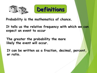
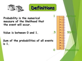
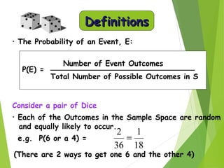
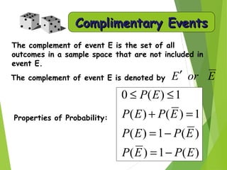
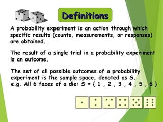
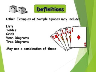
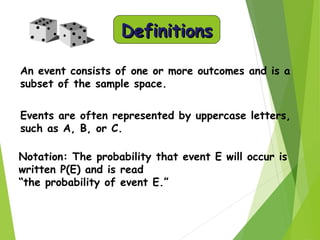
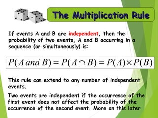
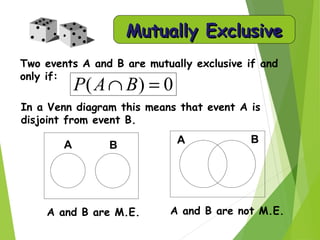
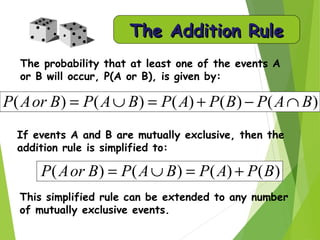
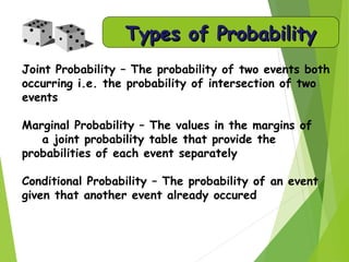
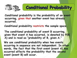
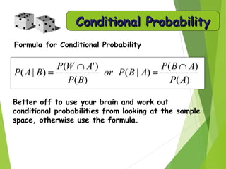
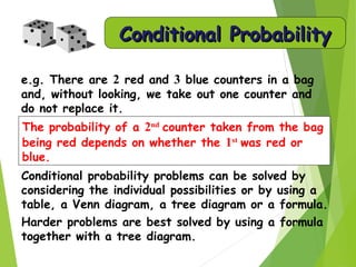
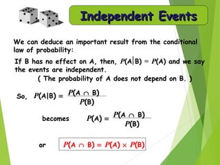
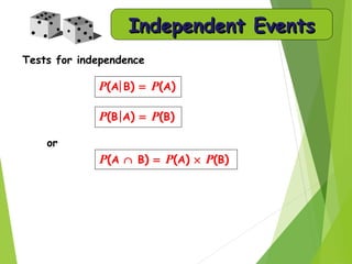
This document defines key concepts in probability, including: - Probability is a measure of the likelihood of an event occurring, represented as a value between 0 and 1. - A probability experiment contains a sample space of all possible outcomes, and events are subsets of outcomes. - Rules like addition and multiplication allow calculating probabilities of combined events. - Conditional probability is the likelihood of an event given another event occurred. Independence means one event doesn't impact another. 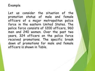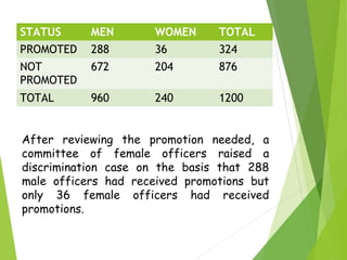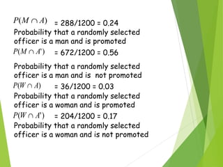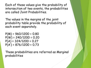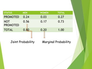- An example uses joint, marginal, and conditional probabilities to analyze officer promotions data.

1. Applicable MathematicsApplicable Mathematics
“Probability”“Probability”
By-
Chaitanya Lakshmi devi
Yoga Lakshmi

2. DefinitionsDefinitions
Probability is the mathematics of chance.
It tells us the relative frequency with which we can
expect an event to occur
The greater the probability the more
likely the event will occur.
It can be written as a fraction, decimal, percent,
or ratio.

3. DefinitionsDefinitions
Certain
Impossible
.5
1
0
50/50
Probability is the numerical
measure of the likelihood that
the event will occur.
Value is between 0 and 1.
Sum of the probabilities of all events
is 1.

4. DefinitionsDefinitions
A probability experiment is an action through which
specific results (counts, measurements, or responses)
are obtained.
The result of a single trial in a probability experiment
is an outcome.
The set of all possible outcomes of a probability
experiment is the sample space, denoted as S.
e.g. All 6 faces of a die: S = { 1 , 2 , 3 , 4 , 5 , 6 }

5. DefinitionsDefinitions
Other Examples of Sample Spaces may include:
Lists
Tables
Grids
Venn Diagrams
Tree Diagrams
May use a combination of these

6. DefinitionsDefinitions
An event consists of one or more outcomes and is a
subset of the sample space.
Events are often represented by uppercase letters,
such as A, B, or C.
Notation: The probability that event E will occur is
written P(E) and is read
“the probability of event E.”

7. DefinitionsDefinitions
• The Probability of an Event, E:
Consider a pair of Dice
• Each of the Outcomes in the Sample Space are random
and equally likely to occur.
e.g. P(6 or a 4) =
(There are 2 ways to get one 6 and the other 4)
P(E) =
Number of Event Outcomes
Total Number of Possible Outcomes in S
18
1
36
2
=

8. Complimentary EventsComplimentary Events
The complement of event E is the set of all
outcomes in a sample space that are not included in
event E.
The complement of event E is denoted by
Properties of Probability:
EorE′
)(1)(
)(1)(
1)()(
1)(0
EPEP
EPEP
EPEP
EP
−=
−=
=+
≤≤

9. The Multiplication RuleThe Multiplication Rule
If events A and B are independent, then the
probability of two events, A and B occurring in a
sequence (or simultaneously) is:
This rule can extend to any number of independent
events.
)()()()( BPAPBAPBandAP ×=∩=
Two events are independent if the occurrence of the
first event does not affect the probability of the
occurrence of the second event. More on this later

10. Mutually ExclusiveMutually Exclusive
Two events A and B are mutually exclusive if and
only if:
In a Venn diagram this means that event A is
disjoint from event B.
A and B are M.E.
0)( =∩ BAP
A BA B
A and B are not M.E.

11. The Addition RuleThe Addition Rule
The probability that at least one of the events A
or B will occur, P(A or B), is given by:
If events A and B are mutually exclusive, then the
addition rule is simplified to:
This simplified rule can be extended to any number
of mutually exclusive events.
)()()()()( BAPBPAPBAPBorAP ∩−+=∪=
)()()()( BPAPBAPBorAP +=∪=

12. Types of ProbabilityTypes of Probability
Joint Probability – The probability of two events both
occurring i.e. the probability of intersection of two
events
Marginal Probability – The values in the margins of
a joint probability table that provide the
probabilities of each event separately
Conditional Probability – The probability of an event
given that another event already occured

13. Example
Let us consider the situation of the
promotion status of male and female
officers of a major metropolitan police
force in the eastern United States. The
police force consists of 1200 officers, 960
men and 240 women. Over the past two
years, 324 officers on the police force
received promotions. The specific break
down of promotions for male and female
officers is shown in Table.

14. After reviewing the promotion needed, a
committee of female officers raised a
discrimination case on the basis that 288
male officers had received promotions but
only 36 female officers had received
promotions.
STATUS MEN WOMEN TOTAL
PROMOTED 288 36 324
NOT
PROMOTED
672 204 876
TOTAL 960 240 1200

15. Let
M= event of an officer is a man
W= event of an officer is a women
A= event an officer is promoted
A’= event an officer is not promoted
The police administration argued that
relatively low number of promotions for
female officers was due not to
discrimination, but to the fact that
relatively few females are members of
the police force.

16. )( AMP ∩
)'( AMP ∩
= 288/1200 = 0.24
Probability that a randomly selected
officer is a man and is promoted
= 672/1200 = 0.56
Probability that a randomly selected
officer is a man and is not promoted
)( AWP ∩ = 36/1200 = 0.03
Probability that a randomly selected
officer is a woman and is promoted
)'( AWP ∩ = 204/1200 = 0.17
Probability that a randomly selected
officer is a woman and is not promoted

17. Each of these values give the probability of
intersection of two events, the probabilities
are called Joint Probabilities.
The values in the margins of the joint
probability table provide the probability of
each event separately.
P(M) = 960/1200 = 0.80
P(W) = 240/1200 = 0.20
P(A) = 324/1200 = 0.27
P(A’) = 876/1200 = 0.73
These probabilities are referred as Marginal
probabilities

18. STATUS MEN WOMEN TOTAL
PROMOTED 0.24 0.03 0.27
NOT
PROMOTED
0.56 0.17 0.73
TOTAL 0.80 0.20 1.00
Joint Probability Marginal Probability

19. Conditional ProbabilityConditional Probability
Conditional probability is the probability of an event
occurring, given that another event has already
occurred.
Conditional probability restricts the sample space.
The conditional probability of event B occurring,
given that event A has occurred, is denoted by P(B|
A) and is read as “probability of B, given A.”
We use conditional probability when two events
occurring in sequence are not independent. In other
words, the fact that the first event (event A) has
occurred affects the probability that the second
event (event B) will occur.

20. Conditional ProbabilityConditional Probability
Formula for Conditional Probability
Better off to use your brain and work out
conditional probabilities from looking at the sample
space, otherwise use the formula.
)(
)(
)|(
)(
)'(
)|(
AP
ABP
ABPor
BP
AWP
BAP
∩
=
∩
=

21. Conditional probability problems can be solved by
considering the individual possibilities or by using a
table, a Venn diagram, a tree diagram or a formula.
Harder problems are best solved by using a formula
together with a tree diagram.
e.g. There are 2 red and 3 blue counters in a bag
and, without looking, we take out one counter and
do not replace it.
The probability of a 2nd
counter taken from the bag
being red depends on whether the 1st
was red or
blue.
Conditional ProbabilityConditional Probability

22. We can deduce an important result from the conditional
law of probability:
( The probability of A does not depend on B. )
or P(A ∩ B) = P(A) × P(B)
If B has no effect on A, then, P(A B) = P(A) and we say
the events are independent.
becomes P(A) =
P(A ∩ B)
P(B)
P(A|B) =So, P(A ∩ B)
P(B)
Independent EventsIndependent Events

23. Tests for independence
P(A ∩ B) = P(A) × P(B)
P(A B) = P(A)
or
Independent EventsIndependent Events
P(B A) = P(B)

24. THANK YOUTHANK YOU