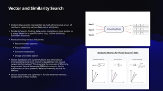
The document discusses the integration of the pgvector extension with PostgreSQL for vector similarity search, detailing its functionalities compared to dedicated vector databases like Pinecone. It outlines various use cases highlighting challenges and proposed methods for enhancing recommendation systems and handling dissimilarity constraints in search results. Additionally, it examines the technical aspects of pgvector, including its data types, indexing strategies, and mechanisms for optimizing performance in vector queries.

1. PgVector + :
Enable Richer
Interaction with
vector database
Ayush Ranjan

2. Today’s Agenda
• Intro to Vector and Similarity
• Intro to Postgres Extension
• Intro to pgVector
• Why not dedicated vector databases like PineCone ?
• Motivation
• UseCase 1 and its proposed solution
• UseCase 2 and its proposed solution
• UseCase 3 and its proposed solution
• UseCase 4 and its proposed solution
• Lesson Learnt and future scope
• References and links to explore

3. Vector and Similarity Search
• Vectors: Data points represented as multi-dimensional arrays of
numbers, capturing various features or attributes.
• Similarity Search: Finding data points (neighbors) most similar to
a query based on a specific metric (e.g., cosine similarity,
Euclidean distance).
• Revolutionizing various industries:
• Recommender systems
• Fraud detection
• Content moderation
• Image and video search
• Vector databases are a powerful tool, but what about
incorporating long-term memory capabilities into neural
networks themselves? This is where the concept of Memory-
Augmented Neural Networks (MANNs) comes in. Vector
databases can be a powerful external memory source for
MANNs.
• Vector databases are a perfect fit for the external memory
component of RAG models.

4. PostGres Extensions
Introduction
• PostgreSQL (PG) is a robust relational database with extensive features, including
SQL standards compliance, support for various extensions, and active community
development.
• PG's flexible, open-source license allows for the development of custom solutions
and integration with third-party vendors.
• PostgreSQL (PG) extensions are add-on modules that enhance the functionality of
the PostgreSQL database system.
• Extensions are installed using the CREATE EXTENSION command in PostgreSQL.
• Four basic file types that are required for building an extension : MakeFile, Control
File,SQL File and Source Code File.

5. PostGres Extension
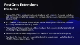
More Information
• Makefile for PostgreSQL Extension:
• Provides instructions for compiling C code, linking it into a shared library, and installing necessary files into
PostgreSQL.
• Relies on "PGXS" infrastructure to simplify building and installing extensions.
• Extension Control File:
• Named [EXTENSION NAME].control.
• Specifies metadata such as name, version, author, module path, and relocatability.
• Extension SQL File:
• Mapping file to link PostgreSQL functions with corresponding C functions.
• Extension C Code:
• Most common language for PostgreSQL extensions due to performance and flexibility.
• Allows direct access to PostgreSQL's internal APIs for optimized functionality.
• Must include PG_MODULE_MAGIC macro for identifying and providing metadata to PostgreSQL about the extension.

6. Introduction
to PgVector
• PgVector is an open-source extension tailored for PostgreSQL,
specifically engineered to streamline vector similarity search
operations. It equips users with the ability to store and query
vector data, which serves as a fundamental component in
numerous machine learning and artificial intelligence
applications.
• Harnessing the robust querying capabilities, data security
features, and extensive ecosystem of tools and libraries offered
by PostgreSQL, PgVector delivers a flexible and potent solution
for managing vector data.
• PgVector allows you to create UDFs written in languages like C
or PL/pgSQL. These functions can implement custom distance
metrics or vector manipulation logic that extend PgVector's
built-in functionalities.
• PgVector overloads comparison operators like < (less than) and
> (greater than) to work with vector columns. When used in
queries, these operators internally translate to distance metric
calculations (e.g., cosine similarity) between the query vector
and the vectors in the column.
• PgVector leverages PostgreSQL's existing query planning and
optimization techniques to ensure efficient execution of vector-
based queries. This involves analyzing the query, available
indexes, and data distribution to determine the most efficient
execution plan.

7. Internals of PgVector
• It introduces a dedicated data type for vectors and
functions for vector similarity search.
• PgVector supports two main index types: HNSW and
IVFFlat, which prioritize speed over perfect accuracy in
similarity search. These indexes are tailored for efficient
similarity search, allowing you to retrieve vectors most
similar to a given query vector based on specific
distance metrics (e.g., cosine similarity).
• Uses TOAST (The Only As Needed Storage). The large
content from the flagged columns is extracted and
stored in a separate table called a TOAST table. This
table is hidden from users and automatically managed
by PostgreSQL. In the original table, the large columns
are replaced with smaller pointers referencing the
location of the actual data in the corresponding TOAST
table.

8. Why not do vector DB from scratch, rather
than using PostgreSQL?
• Bottleneck in using a closed-source search
solution like Pinecone is primarily the latency
from network requests, not the search
operation itself
• Pinecone does provide scalability through the
adjustment of resources such as vCPU, RAM,
and disk (termed as “pods”)
• Data Synchronization Issues
• Incomplete database solution — lacks row-
level security, database backups, bulk
operations, and complete ACID compliance
• More Info -
PgVector vs Pinecone by supabase ,
Confident AI

9. Motivation
• PgVector, while a valuable PostgreSQL ex-
tension for vector similarity search, lacks certain
essential features compared to other vector
databases, such as scalar quantization. These
features have proven to be efficient for specific
workloads.
• However, all vector databases have inherent
limitations even with these additional features.
o Diversification of Set of Responses to the
Query
o Enabling Similarity and
Dissimilarity Constraint
o Enabling Low-Level Composition of Multiple
Queries
• Overcoming these challenges, vector databases
can become more versatile and effective tools
for various applications.

10. Use Case 1
Diversification of
Set of Responses to
the Query
• In a recommendation system,
users often require a variety of
suggestions rather than exact
matches.
• For instance, if a user is
watching videos of a white cat,
the system should recommend
videos featuring cats of different
colors or species to ensure
diversity in the suggestions.
• This diversification is crucial for
enhancing user engagement
and satisfaction.

11. Method 1:
Naive
Approach
outside
Database
• The Naive approach to diversification involves
expanding the search area beyond the
required number of responses (Top K) by a factor
n, where n takes values like 2, 3, 4, etc and then
randomly selecting or systematically picking
responses, such as selecting every nth element
starting from the first.
• Advantage : This approach is straightforward to
implement, minimal effort to implement. By
expanding the search area, there’s a chance of
discovering new and diverse content that may not
have been included in the top K results.
• Disadvantage : Expanding the search area
increases computational overhead.

12. Method 2:
Naive
Approach
inside
Database
• The database would typically conduct a
similarity search across all vectors, sorting
them and returning the top K results.
• We can modify this process. Instead of
solely returning the top K vectors, we can
perform the same logic on the sorted list
obtained from the database. This means we
can choose to return responses randomly
or by selecting every nth element directly
within the database.
• Advantage : eliminates the overhead
associated with conducting these
operations externally
• Drawback - While this works well when we
do brute force to find similar vectors, it will
not work well if indexes are used to do so
since the data returned by doing so using
index might not contain k elements.

13. Method 3:
With
Indexing( IVF-
FLAT)
• In IVF, clusters are utilized, and we identify the cluster centroid with the
least distance from the query cluster. This is determined by the default
value of probes, which sets the number of clusters to be examined at 1,
thus selecting the cluster with the minimum distance.
• We require input from various clusters. Therefore, we must augment the
number of probes to, let's say, n. Consequently, IVF-Flat will compare all the
vectors within these clusters and generate a sorted list.
• We then could pick every (size of list)/ k elements.
• Although this elevates the computational cost compared to examining just
one cluster as before, it still diminishes the search space in contrast to
operating without indexing.
• Drawback - Finding the optimal "probes" value can be challenging,
balancing diversification and efficiency.

14. Method 4
Diversification
with threshold
• one of the primary challenges we
encountered was determining the
diversity of our results. Simply
increasing the number of probes did
not ensure diversity.
• We explored the idea of implementing
a threshold to classify results as both
similar and diverse if they fell within a
specified range.
• At present, pgvector offers three
distance calculation metrics: Euclidean
Distance, Cosine Distance, and Inner
Product. To ascertain the feasibility of
such a threshold, we need to
investigate these metrics.

15. Euclidean Distance
• Also know as L2 distance
• The threshold could be based on a predefined
maximum acceptable difference between the
two values. For example, if the Euclidean
distance between two points is less than or
equal to the threshold, they could be
considered similar.
• Disadvantages :
o Determining an appropriate threshold can be
subjective and context-dependent. What may be
considered "similar" in one scenario may not be
appropriate in another.
o The Euclidean distance is sensitive to the scale of
the data. Normalization or standardization of the
data may be necessary to address this issue.
o For datasets with many zero or near-zero values
(sparse data), the Euclidean distance may not
effectively capture similarity.

16. Inner Product
• Also known as the scalar product or dot product
• It is calculated by multiplying corresponding components
of the vectors and then summing up the results.
• For the dot product, the range of possible values
depends on the vectors being multiplied.
• Positive values indicate the vectors are in the same
direction, negative values that they are in opposite
directions, and 0 are orthogonal.
• Disadvantages :
o Positive dot product values may exhibit varying
ranges depending on the dataset. Consequently,
identifying a single threshold value becomes
complex in such scenarios.
o The effectiveness of a threshold may vary
depending on the variability of the data and the
specific characteristics of the vectors being
compared.

17. Cosine Similarity
• It calculates the cosine of the angle between the two vectors
• The cosine similarity ranges from -1 to 1 :
o A value of 1 indicates that the vectors are perfectly similar, meaning they are pointing in the
same direction.
o A value of -1 indicates they are perfectly dissimilar, meaning they are pointing in opposite
directions.
o A value of 0 indicates orthogonality (perpendicular), meaning the vectors are at right angles
to each other.
• We can adopt a threshold-based approach. This approach entails
leveraging cosine similarity with three distinct modes, each characterized
by its unique threshold range, to classify similarity levels among pairs of
vectors. These modes are outlined as follows:
o Strict Mode (Threshold: 0.5 to 0.75) - It indicates a moderately diverse result set, allowing for
some level of similarity but also room for diversity.
o Moderate Mode (Threshold: 0.75 to 0.9)- It represents a less diverse set compared to strict
mode, implying a higher degree of similarity among the pairs.
o Limited Mode (Threshold: 0.9 to 1)- It denotes very similar result sets, where the cosine
similarity is close to 1, indicating a high level of similarity between the pairs.
• The approach provides a finer-grained classification of similarity levels by
dividing the cosine similarity scores into three distinct modes.
Furthermore, adjusting threshold ranges in each mode offers
customization and flexibility based on specific use cases and preferences.

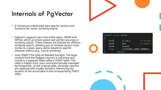
18. Using
threshold
outside
database vs
Inside
• Currently, pgvector provides functionality for
comparing vector similarity distances.
• As per the documentation, a query such as SELECT
* FROM items WHERE embedding <-> '[3,1,2]' < 5;
can be utilized to retrieve all vectors with distances
smaller than 5 from the specified query vector.
• Utilizing a keyword within the database as an
alternative approach to performing the same
process is feasible but won't add any performance
benefit.
• Use Iterative Search to add values to result set if in
case we don't get top K vectors.
• Conclusion : Employing a library that harnesses
SQL queries would deliver comparable accuracy
without the need for introducing a new keyword.
Opting for such a library not only ensures ease of
comprehension and implementation but also
leverages pgvector's optimized distance
calculations. Moreover, it offers flexibility as
threshold adjustments necessitate only query
modifications, minimizing the performance impact
caused by frequent changes.

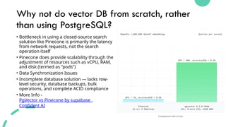
19. Use Case 2
Enabling Similarity
and Dissimilarity
Constraint
• Another limitation of current vector
databases is the inability to
handle dissimilarity constraints
• A search query like ”Places without
snow” may not be accurately
interpreted by the vectors, as
neural models often struggle with
encoding negations and
nuances, as mentioned in various
research papers such as [1]
• To address this, databases should
incorporate features that should
be able to find dissimilarity, thereby
improving the accuracy of search
results.

20. Method 1:
Dissimilarity
using
threshold
• For dissimilar images, a cosine value of -1 indicates that the
vector lies in the opposite plane of the query vector.
• For instance, if we consider a scenario with 100 vectors in
our database and none of them exactly matches a cosine
similarity of 1, the query would return empty results.
• A potential workaround involves employing modes similar to
our previous exploration. These modes could be categorized
as follows: "Strict" indicating cosine = -1, "Moderate"
encompassing values from -0.75 to -1, and "Limited" ranging
from -0.5 to -0.75.
• However, a significant challenge with this approach lies in
determining the appropriate threshold values and ensuring
that they guarantee retrieval of the desired number of
elements (k).
• Another issue is the use of indexing. We can't use the
existing indexes for dissimilarity even if we use
Iterative Search.
• The threshold approach poses another challenge in terms of
computational cost.

21. Method 2:
Dissimilarity
Constraint in
Database
• Let's first explore how we can adapt the brute force approach
to achieve this goal.
o when searching for the top K similar elements, the typical process
involves iterating through all data points, calculating the similarity score
for each
o sorting these scores, and finally returning the top K elements
o for dissimilarity, we can simply select the last K elements after sorting.
• We can leverage indexing and aim to refine the existing
indexing(IVF-FLAT) approach with some adjustments.
o IVF-Flat groups vectors stored in the database into distinct clusters, with
each cluster characterized by a centroid representing the average of all
data points within it.
o When a query vector is received, its distance is computed with respect to
these cluster centroids.
o Instead of selecting the minimum 'n' clusters as in the original approach,
we prioritize the maximum 'n' clusters. This means we prioritize clusters
that exhibit the greatest distance from the query vector.
o Following this selection, a brute force approach is applied to the
elements within the chosen clusters.
o There's a crucial modification in the sorting process: while initially, the
elements were sorted in ascending order based on distance, now, with
the dissimilarity constraint, the sorting is done in descending order.

22. Implementation Concept
• To implement the necessary changes in the code flow of pgvector, utilizing the
Postgres Indexing API, we'll focus on the IndexAmRoutine API
• These changes will align the code flow with the dissimilarity constraint, ensuring
that indexing operations select clusters based on maximum distance and sort the
elements within these clusters in descending order.
• Update Sorting Criteria:
o Modify the ivfflatbeginscan method within the IndexAmRoutine API.
o Replace Float8LessOperator with Float8gt to sort in descending order.
• Adjust Cluster Selection:
o In the amgettuple method, which retrieves the next valid tuple, adjust the
heap maintained to store elements.
o Set the value of min_diff to _DBL_MAX to ensure maximum distance
comparison.
o Reverse the if condition to check if distance > maxDistance.
• Conclusion : Create a new index with different name IVF_Flat_Dissimilar with all
the code of IVF_FLAT with the above mentioned changes, then query the database
with CREATE INDEX ON items USING ivfflat_dissimilar (embedding
vector_l2_ops) WITH (lists = 100);

23. Bonus Method
• PgVector stores the negative dot product as the
distance in the result vector.
• To use the IVFFLAT index effectively, pgvector needs to
convert the similarity measure (dot product) into a
dissimilarity measure (distance). It achieves this by
negating the dot product. So, a larger negative value
(more negative dot product) indicates greater
dissimilarity (vectors are further apart) which aligns well
with the IVFFLAT indexing approach.
• We could levarage this by storing the dot product
as distance in the result vector. In this case we just need
to add one more distance calculation method. This
would be most effective but there is no formal
proof that I found, given the time constraint.

24. Use Case 3
Enabling Low-Level
Composition of
Multiple Queries
• In real-world scenarios, single-query searches may not
always suffice. Consider a situation where one needs
to search for images similar to both image A and
image B simultaneously. However, the current system
lacks support for such multi-image search operations.
• The workaround involves conducting separate query
searches and merging the results
o let's say we have three vectors: vector 1 representing
"USA," vector 2 representing "Basketball," and vector 3
representing "team."
o we would retrieve the top k vectors similar to each of
these individual vectors.
o based on certain criteria, elements from each set might
be selected.
• A significant issue with this method is that even if we
do find these vectors, it does not guarantee relevance
to the concept of "USA Basketball Team" as a whole; it
merely identifies vectors related to individual words.
• The next approach would be instead of vector get the
original data and then append those data pass it to
deep learning model and get the vector embedding .
Now use this vector embedding to do similarity search.
• But even with that it still requires us to have the
original data. Can we do something similar with
vectors?

25. Method 1:
Using
centroid
approach for
set of vectors • To understand how centroid should be calculated, we should look into the implementation of IVF-FLAT of pgvector i.e. IvfflatKmeans method
• The function IvfflatKmeans takes three arguments:
o index: This relates to the specific Post-greSQL index being used for the k-means clustering
o samples: This is a vector array containing the data points to be clustered
o centers: This is a vector array that will store the centroids (cluster centers) to be found
• The function first checks if there are enough data points (samples) to create the desired number of centroids (centers). If not, it uses a simplified approach (QuickCenters) to select centroids.
• Here's a summary of the steps involved in the QuickCenters function:
o Sorting and Avoiding Duplicates:
▪ The function sorts the samples array based on their vector components.
• This sorting ensures that centroids are chosen from diverse regions of the data space.
• It iterates through the sorted samples array, adding each unique data point to the centers array until the desired number of centroids (specified by centers->maxlen) is reached
▪ The centroids are iteratively updated by calculating the mean of the data points assigned to each centroid. This process continues until a convergence criterion is met (e.g., no significant changes in centroid positions).
o Normalization (optional):
▪ The code checks if an optional normalization procedure is defined for the k-means process (Ivf-flatOptionalProcInfo).
▪ If so, it applies the normalization function to each randomly generated centroid vector.
▪ Normalization can be important for distance metrics like cosine similarity, where the magnitude of the vector affects the similarity score
o Filling with Random Data (if needed):
▪ If there are still empty slots in the centers array after processing all unique data points, the function fills them with randomly generated data points.

26. Method 1:
Using
centroid
approach for
set of vectors
• Calculating the mean of vectors can be an effective method for combining vectors
• This approach has been previously employed to generate vector embeddings of sentences, particularly
before the widespread adoption of deep learning models, where methods like word2vec were utilized to
create embeddings of individual words.
• This approach has proven to be effective and can be leveraged to identify similar vectors in comparison to a
given set of vectors
• Drawbacks of Centroid Method
o Outliers in the data can significantly influence the mean calculation, potentially skew-ing the combined
vector away from the central tendency of the data.
o Mean calculation assumes that all vectors contribute equally to the combined result. However, in many cases, certain
vectors may be more relevant or significant than others
• Other potential variations
o Minimum Value Selection
▪ Consider having three vectors, each with three dimensions.
• One approach is to select the minimum value among these three vectors in each dimension.
• This results in a strict match, as the resultant vector contains the minimum values required from each
dimension.
▪ Subsequently, a similarity search can be performed based on this combined query vector.
o Maximum Value Selection
▪ Another variation of this approach is to select the maximum value in each dimension to create the combined
query vector.
• While both methods may seem more stringent compared to averaging, their effectiveness depends on the
specific use case.

27. How to validate choices ?
• Further analysis is required to validate earlier hypothesis
and determine the most suitable approach for the given
scenario.
• Library Development:
o Implementing these methods directly in the
database would require substantial effort.
o A more efficient approach would be to create a
library to check the effectiveness of each method.
o Once the library is developed, thorough exploration
can be conducted to determine the best approach
for the given scenario.

28. Method 2:
Custom
Searching
• Individual Similarity Search
o Conduct a similarity search with each individual vector in the database.
o Track the distance of each vector in the database from each query vector.
• Combined Vector Distance Representation
o To represent the combined vector distance, compute the average of all the distance vectors.
• Sorting Based on Combined Distance
o This can incorporate the different weights associated with vectors
• Since the distance are maintained in database and discarded once the query is completed, an ideal
place to do this change in inside the database system.
• Two implementation approach can be explored here
o Inside pgvector by modifying the code
o Create a custom PL/pgSQL function named search_similar_vectors within your PostgreSQL
database which would work on top of pgvector

29. What is
PL/psSQL ?
• PL/pgSQL is a procedural language extension for PostgreSQL that enables the creation of custom
functions directly within the database. These functions are written using SQL commands, control
structures, and procedural language constructs, providing a powerful tool for developing complex
database logic.
• PL/pgSQL functions seamlessly integrate with SQL commands, allowing developers to execute SQL
queries within the function body.
• PL/pgSQL functions support parameterized inputs, allowing developers to define input parameters that
can be used to customize the behavior of the function. These parameters can be of various data types,
including scalar types, composite types, and arrays, providing flexibility in function usage.
• PL/pgSQL functions execute within the security context of the PostgreSQL database, adhering to the
access privileges and permissions defined for the database objects. This ensures data security and
integrity while executing the function.
• Implementation with PL/pgSQL:
o Write the provided PL/pgSQL code within a text editor.
o Use the CREATE FUNCTION statement in PostgreSQL to define the function with its
arguments, return type, and the PL/pgSQL code body.
o Once created, you can call the search_similar_vectors function from within your SQL queries,
specifying the query vectors and index name.

30. Implementation of
PL/pgSQL function
• Input:
o query_vectors: A pgvector array containing the set of query vectors
for which you want to find similar vectors.
o index_name: The name of the PostgreSQL index that uses pgvector
for similarity search.
• Process:
o Fetches database vectors from the specified table using the provided
index.
o Loops through each query vector:
o Calculates the distance between the current query vector and all
database vectors using pgr_distance.
o Accumulates these distances for each database vector in a
combined_distances array.
o Calculates the average distance for each database vector by dividing
the accumulated distance by the total number of query vectors.
o Sorts the database vectors based on their average distance
(ascending order), with closer average distances indicating greater
similarity to the query vectors.
• Output:
o The function returns the sorted database vector array, providing the
most similar vectors first based on their average distance to the
query set

31. UseCase 4:
Scalar
Quantization
• Quantization is the process of reducing the number of distinct values (or levels of precision) used
to represent data.
• It involves mapping a continuous range of values to a finite set of discrete values. Commonly
used in data compression, image and video coding, and various signal processing applications.
• Quantization in the Context of Vectors:
o Refers to the process of reducing the number of distinct values or levels used to represent
each component of a vector.
o Vectors typically have high dimensions, such as the 568 and 768 dimensions commonly
used in models like CLIP and Dinov2.
o Representing these vectors as floating-point numbers requires a significant amount of
memory.
o Each component of vectors is represented as a floating-point number, requiring 32 bits for
representation.
• pgvector currently lacks support for quantization methods. There are open issues regarding the
implementation of quantization in pgvector.

32. Where to use
Quantisation ?
• Should we do quantization when we save the data ?
o Initial intuition involved adjusting the existing structure of pgvector to accommodate an integer
array alongside the float array.
o The current struct for vectors in pgvector was considered, but this approach appeared
impractical due to extensive changes required.
o Another option considered was storing quantized data in separate tables or blob storage
linked to the original vectors.
o While this approach could be implemented with less effort, it ultimately defeats the purpose of
quantization, as the original data would still be retained.
o Overall, the idea of storing quantized vectors instead of original vectors may not be feasible
for various scenarios since Quantization is a lossy technique, and there are scenarios such as
face recognition where accuracy is crucial.
• Is it feasible to employ quantisation in indexing to mitigate storage expenses?
o IVF FLAT Stores the original vector data, offering high accuracy for searches but requiring
more storage.
o Scalar Quantization (SQ) with IVF_FLAT method reduces storage space further by converting
each dimension (value) in the original vector to a smaller data type (e.g., from float to byte).
This significantly reduces the index size.
o create a new index which would support quantization? Why new ? Since there is an accuracy
loss with these quantization based search.

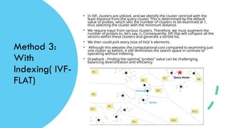
33. How to do Scalar
Quantisation ?
• There are few vector databases which have these functionality such as Zilliz and Qdrant.
Apart from these, Milvus, which is also a vector database offers the scalar quantization
functionality as an index i.e. IVF_SQ8
• Qdrant
o There example shows that 99 percentage of the values come from a [-2.0, 5.0]
range
o So accordingly they derived the equation.
o Both parameters, namely offset and alpha, must be calculated for a given set of
vectors. This can be achieved by substituting the minimum and maximum of the
represented range for both f32 and i8. By substituting the maximum over minimum
in place of alpha, we obtain two equations to calculate the offset.
• Zilliz
o Take the maximum and minimum value of that particular dimension across the
database.
o Split the dimension into bins across the range. To create bins, we use two variables:
▪ Start = Min Value
▪ Steps = (Max Value - Min Value) / 255, where 255 is the integer range.
o Subtract the minimum value from each vector, divide by 255, and place vectors in
these bins.

34. Which
approach to
choose?
• There is no comparision of these as of now so deciding on which to pick would be difficult.
• Stumbled upon a paper by
Google “Accelerating Large-Scale Inference with Anisotropic Vector Quantization ” which is also
used by Google's ScaNN library
• I believe Zilliz also took reference from this paper although they haven't mentioned about
anything.
• Steps:
o Specify the minimum and maximum values of the input signal.
o Choose the number of quantization levels: 2^number of bits (2^8 = 256 for 8-bit
quantization).
o Techniques like uniform or Lloyd-Max quantization can be used to distribute the levels
across the range.
▪ In uniform quantization, the range of values is divided into equal intervals. The
width of each interval is determined by dividing the range of values by the desired
number of quantization levels.
▪ Lloyd-Max quantization algorithm begins with an initial set of quantization levels,
often evenly spaced across the range of values. In each iteration, the algorithm
performs the following steps:
• Assign each input value to the nearest quantization level.
• Update the quantization levels by computing the centroid of the values
assigned to each level.
• Check for convergence by measuring the change in the quantization levels
between iterations.
o Assign each input value to the closest quantization level, represented by an 8-bit binary
code (0 to 255).

35. Implementation
Concept
• Establish a distinct set of distance functions tailored for
these quantized vectors.
• Register these functions as supplementary support
functions for the access method.
• Allow users to designate WITH (quantizer = 'BQ') when
creating an index on a vector column to indicate the
use of quantization.
• Expand the strategy to enable users to store quantized
vectors directly in the table, utilizing the chosen data
type. Ensure that the same set of distance functions is
utilized for both indexed quantized vectors and directly
stored quantized vectors.
• Optimize performance for various scenarios by
implementing these changes in pgvector to enable
efficient storage and indexing of quantized vectors.

36. Implementation
Concept
• ScalarQuantizeVector method
o Parameters:
▪ const Vector* in: The input vector to be quantized.
▪ const Vector* multipliers: Multipliers used for quantization.
▪ bytea* quantized_storage: Storage for storing quantized values.
o Iterates over each component of the input vector. Multiplies each component with the corresponding
multiplier.
o Rounds the result to the nearest integer and stores it in quantized_storage. Handles cases where the
result exceeds the range of int8_t.
o Returns a pointer to quantized_storage
• Dot Product Distance:
o Parameters:
▪ const Vector* preprocessed_query: The preprocessed query vector.
▪ const TupleDesc tuple_desc: The tuple descriptor of tuples in the page.
▪ const Page page: Pointer to the page containing vectors.
▪ Vector* result: Pointer to store the computed distances.
o Iterates over each vector in the page. Computes the dot product between the preprocessed query vector
and each vector in the page
o Stores the negative dot product as the distance in the result vector.

37. IVF Build Phase
Quantizer
Initialization:
Determine the type of
quantizer using
IvfGetQuantizer(index)
and store it in
buildstate->quantizer.
Perform initialization
steps specific to kIvfflat
if that quantizer type is
detected.
Perform initialization
steps specific to kIvfsq8
if that quantizer type is
detected.
Throw an error if the
quantizer type is neither
kIvfflat nor kIvfsq8.
Memory Allocation:
Allocate memory for
buildstate->multipliers
and buildstate-
>quantized_storage
based on the quantizer
type.
Initialize buildstate-
>multipliers with zero
values and allocate
memory for buildstate-
>quantized_storage
based on index
dimensions if the
quantizer type is
kIvfsq8.
Memory
Deallocation:
Free buildstate-
>multipliers and
buildstate-
>quantized_storage if
they were previously
allocated to prevent
memory leaks.
Setting Page
Header:
Adjust the page header
(((PageHeader)page)-
>pd_lower) to
accommodate metadata
or multipliers based on
the quantizer type
Creating IVF List:
Create an IVF list (list)
based on the index and
associated metadata.
Allocate memory for the
list and set its
properties based on the
provided parameters.

38. IVF Insert Phase
Index Tuple
Formation
Form an index tuple from a raw vector in
its scalar 8-bit quantized form.
Compute the quantized vector using
scalar quantization with the multipliers
retrieved from the index.
Allocate memory for the quantized vector
storage and set its size.
Form the index tuple using the computed
quantized vector.
Free the allocated memory after forming
the index tuple.
Processing Index List
Retrieve each item (list) from a page in
the index.
Extract metadata associated with the list
and flatten it if it's stored externally.
Calculate the distance metric using the
flattened metadata and a specified
function.
Handling Quantizers
Determine the quantizer type used in the
relation.
If the quantizer is scalar 8-bit, form the
index tuple using the quantized vector.
If the quantizer is flat, form the index
tuple directly from the raw vector.
Throw an error if the quantizer type is
not supported.

39. • Create a new index while retaining the existing
IVFFLAT index. This allows users to choose between
using the IVFFLAT index or the new quantized
version.
• IVFFLAT Index Usage
o CREATE INDEX ON items USING ivf (lists=100);
• New Quantized Version Usage
o CREATE INDEX ON items USING ivf (lists=100,
quantizer='SQ8');

40. • Pgvector is a great extension which helps you
use postgres as vector database which has all
the features of a vector database and utilizes the
strong infrastructure of postgres.
• Learnt about internal of postgres, internals
indexing uses in pgvector , PL/pgSQL, vector
manipulation
• Few Open points
o To validate/ test the finding we need a proper dataset
and models.
o Testing of approaches of Use Case 3 using library
extension as well as PL/pgSQL
o Enabling Different Matrix to Self-Similarity for
Responses
o Binary Quantisation
o Dive into HSNW index implementation and it's usage
in these usecases.
Lesson Learnt and Future Scope

41. References And Further links to explore
• https://www.postgresql.org/docs/current/extend-pgxs.html
• https://www.postgresql.org/docs/current/index-functions.html
• Pgvector - https://github.com/pgvector/pgvector
• Quatization https://www.elastic.co/search-labs/blog/articles/scalar-quantization-101,
https://zilliz.com/learn/scalar-quantization-and-product-quantization,
https://qdrant.tech/documentation/guides/quantization/,
https://arxiv.org/pdf/1908.10396.pdf
• PCA - A SIMPLE BUT TOUGH-TO-BEAT BASELINE FOR SEN- TENCE EMBEDDINGS ,
All-but-the-Top: Simple and Effective Postprocessing for Word Representations,
Effective Dimensionality Reduction for Word Embeddings
• Distance Metrics - https://www.youtube.com/watch?v=e9U0QAFbfLI,
https://www.learndatasci.com/glossary/cosine-similarity/ ,
https://en.wikipedia.org/wiki/Euclidean_distance,
https://tivadardanka.com/blog/how-the-dot-product-measures-similarity, Take this QUIZ

42. Thank You !!!