PajekManual

Pajek
Program for Analysis and
Visualization of Large Networks

Reference Manual
List of commands with short explanation
version 2.00

Vladimir Batagelj and Andrej Mrvar

Ljubljana, September 26, 2010

c 1996, 2010 V. Batagelj, A. Mrvar. Free for noncommercial use.
PdfLaTex version October 1, 2003

Vladimir Batagelj
Department of Mathematics, FMF
University of Ljubljana, Slovenia
http://vlado.fmf.uni-lj.si/
vladimir.batagelj@fmf.uni-lj.si

Andrej Mrvar
Faculty of Social Sciences
University of Ljubljana, Slovenia
http://mrvar.fdv.uni-lj.si/
andrej.mrvar@fdv.uni-lj.si

Contents
1 Pajek 3

2 Data objects 6

3 Main Window Tools 8
3.1 File . . . . . . . . . . . . . . . . . . . . . . . . . . . . . . . . . 8
3.2 Net . . . . . . . . . . . . . . . . . . . . . . . . . . . . . . . . . 12
3.3 Nets . . . . . . . . . . . . . . . . . . . . . . . . . . . . . . . . . 31
3.4 Operations . . . . . . . . . . . . . . . . . . . . . . . . . . . . . 33
3.5 Partition . . . . . . . . . . . . . . . . . . . . . . . . . . . . . . 42
3.6 Partitions . . . . . . . . . . . . . . . . . . . . . . . . . . . . . . 43
3.7 Vector . . . . . . . . . . . . . . . . . . . . . . . . . . . . . . . . 44
3.8 Vectors . . . . . . . . . . . . . . . . . . . . . . . . . . . . . . . 45
3.9 Permutation . . . . . . . . . . . . . . . . . . . . . . . . . . . . 46
3.10 Permutations . . . . . . . . . . . . . . . . . . . . . . . . . . . . 47
3.11 Cluster . . . . . . . . . . . . . . . . . . . . . . . . . . . . . . . 47
3.12 Hierarchy . . . . . . . . . . . . . . . . . . . . . . . . . . . . . . 47
3.13 Options . . . . . . . . . . . . . . . . . . . . . . . . . . . . . . . 48
3.14 Info . . . . . . . . . . . . . . . . . . . . . . . . . . . . . . . . . 51
3.15 Tools . . . . . . . . . . . . . . . . . . . . . . . . . . . . . . . . 52

4 Draw Window Tools 55
4.1 Main Window Draw Tool . . . . . . . . . . . . . . . . . . . . . . 55
4.2 Layout . . . . . . . . . . . . . . . . . . . . . . . . . . . . . . . 55
4.3 Layers . . . . . . . . . . . . . . . . . . . . . . . . . . . . . . . . 57
4.4 GraphOnly . . . . . . . . . . . . . . . . . . . . . . . . . . . . . 59
4.5 Previous . . . . . . . . . . . . . . . . . . . . . . . . . . . . . . . 59
4.6 Redraw . . . . . . . . . . . . . . . . . . . . . . . . . . . . . . . 59
4.7 Next . . . . . . . . . . . . . . . . . . . . . . . . . . . . . . . . . 59
4.8 ZoomOut . . . . . . . . . . . . . . . . . . . . . . . . . . . . . . 59
4.9 Options . . . . . . . . . . . . . . . . . . . . . . . . . . . . . . . 59
4.10 Export . . . . . . . . . . . . . . . . . . . . . . . . . . . . . . . 63
4.11 Spin . . . . . . . . . . . . . . . . . . . . . . . . . . . . . . . . . 66
4.12 Move . . . . . . . . . . . . . . . . . . . . . . . . . . . . . . . . 66
4.13 Info . . . . . . . . . . . . . . . . . . . . . . . . . . . . . . . . . 66

5 Exports to EPS/SVG/X3D/VRML 68
5.1 Defaults . . . . . . . . . . . . . . . . . . . . . . . . . . . . . . . 68
5.2 Parameters in EPS, SVG, X3D, and VRML Defaults Window . . . 68

1

5.3 Exporting pictures to EPS/SVG – defining parameters in input file 72
5.4 Using Unicode in Pajek’s pictures . . . . . . . . . . . . . . . . . 76

6 Using Macros in Pajek 79
6.1 What is a Macro? . . . . . . . . . . . . . . . . . . . . . . . . . . 79
6.2 How to record a Macro? . . . . . . . . . . . . . . . . . . . . . . 79
6.3 How to execute the Macro? . . . . . . . . . . . . . . . . . . . . . 79
6.4 Example . . . . . . . . . . . . . . . . . . . . . . . . . . . . . . . 79
6.5 List of macros available in installation file . . . . . . . . . . . . . 80
6.5.1 Macros prepared for genealogies and other acyclic networks 80
6.5.2 Macros prepared for computing derived kinship relations . 81
6.6 Repeating last command . . . . . . . . . . . . . . . . . . . . . . 81

7 Blockmodeling in Pajek 83
7.1 MDL files . . . . . . . . . . . . . . . . . . . . . . . . . . . . . . 83
7.2 Examples of MDL files . . . . . . . . . . . . . . . . . . . . . . . 85
7.2.1 Regular blocks . . . . . . . . . . . . . . . . . . . . . . . 85
7.2.2 Diagonal blocks (clustering) . . . . . . . . . . . . . . . . 85
7.2.3 Acyclic model (up) . . . . . . . . . . . . . . . . . . . . . 85
7.2.4 Acyclic model with symmetric clusters (down) . . . . . . 85
7.2.5 Center-Periphery . . . . . . . . . . . . . . . . . . . . . . 86
7.2.6 Regular path . . . . . . . . . . . . . . . . . . . . . . . . 86
7.2.7 Regular chain . . . . . . . . . . . . . . . . . . . . . . . . 86
7.2.8 2-mode ’standard model’ for Davis.net . . . . . . . . . . 87

8 Colors in Pajek 88

9 Citing Pajek 90

2

Pajek– Manual 3

1 Pajek
Pajek is a program, for Windows, for analysis and visu-
alization of large networks having some thousands or even
millions of vertices. In Slovenian language the word pa-
jek means spider. The latest version of Pajek is freely
available, for noncommercial use, at its home page:
http://vlado.fmf.uni-lj.si/pub/networks/pajek/
We started the development of Pajek in November 1996. Pajek is im-
plemented in Delphi (Pascal). Some procedures were contributed by Matjaˇ Za- z
verˇnik.
s
The main motivation for development of Pajek was the observation that
there exist several sources of large networks that are already in machine-readable
form. Pajek should provide tools for analysis and visualization of such net-
works: collaboration networks, organic molecule in chemistry, protein-receptor
interaction networks, genealogies, Internet networks, citation networks, diffusion
(AIDS, news, innovations) networks, data-mining (2-mode networks), etc. See
also collection of large networks at:
http://vlado.fmf.uni-lj.si/pub/networks/data/
The design of Pajek is based on our previous experiences gained in devel-
opment of graph data structure and algorithms libraries Graph and X-graph, col-
lection of network analysis and visualization programs STRAN, RelCalc, Draw,
Energ, and SGML-based graph description markup language NetML.
http://vlado.fmf.uni-lj.si/pub/networks/default.htm

Figure 1: Pajek/Spider

V. Batagelj and A. Mrvar Pajek 2.00 / September 26, 2010

4 Pajek– Manual

global
hierarchy

local
reduction

inter-links
cut-out context

Figure 2: Approaches to deal with large networks

The main goals in the design of Pajek are:

• to support abstraction by (recursive) decomposition of a large network into
several smaller networks that can be treated further using more sophisticated
methods;
• to provide the user with some powerful visualization tools;
• to implement a selection of efﬁcient (subquadratic) algorithms for analysis
of large networks.

With Pajek we can: ﬁnd clusters (components, neighbourhoods of ‘impor-
tant’ vertices, cores, etc.) in a network, extract vertices that belong to the same
clusters and show them separately, possibly with the parts of the context (detailed
local view), shrink vertices in clusters and show relations among clusters (global
view).
Besides ordinary (directed, undirected, mixed) networks Pajek supports also
multi-relational networks, 2-mode networks (bipartite (valued) graphs – networks
between two disjoint sets of vertices), and temporal networks (dynamic graphs –
networks changing over time).


Pajek– Manual 5

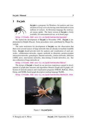
Figure 3: Pajek textbook

This manual provides short explanations of all procedures implemented in the
last version of Pajek. The novice users we advise to read the Pajek textbook
[31]

de Nooy W., Mrvar A., Batagelj V. (2002) Exploratory Social Net-
work Analysis With Pajek. Structural Analysis in the Social Sci-
ences 27, Cambridge University Press, 2005.

For an overview of network analysis with Pajek see the NICTA workshop slides
[5].


6 Pajek– Manual

2 Data objects
In Pajek six types of objects are used:

Figure 4: Pajek’s Main Window

1. Networks – main objects (vertices and lines). Default extension: .net.
Network can be presented on input ﬁle in different ways:
• using arcs/edges (e.g. 1 2 – line from 1 to 2)
• using arcslists/edgeslists (e.g. 1 2 3 – line from 1 to 2 and from 1 to 3)
• matrix format
• UCINET, GEDCOM, chemical formats. . .
Additional information for network drawing can be included in input ﬁle as
well. This is explained in the section Exports to EPS/SVG/VRML.
2. Partitions – they tell for each vertex to which class vertex belong. Default
extension: .clu.
3. Permutations – reordering of vertices. Default extension: .per.
4. Clusters – subset of vertices (e.g. one class from partition). Default exten-
sion: .cls.
5. Hierarchies – hierarchically ordered vertices. Example:

Root
g1 g2
g11 g12 v5,v6,v7
v1,v2 v3,v4


Pajek– Manual 7

Root has two subgroups – g1 and g2. g2 is a leaf – cluster with vertices
v5,v6 and v7. g1 has two subgroups – g11 and g12. . . Default extension:
.hie.

6. Vectors – they tell for each vertex some numerical property (real number).
Default extension: .vec.

By double clicking on selected network, partition,... you can show the object
on screen.
The procedures in Pajek’s main window (see Figure 4) are organized accord-
ing to the types of data objects they use as input.
Permutations, partitions and vectors can be used to store properties of vertices
measured in different scales: ordered, nominal (categorical) and numeric.

Figure 5: Spider web; Photo: Vladimir Batagelj.


8 Pajek– Manual

3 Main Window Tools
3.1 File
Input/Output manipulation with the six data objects.

• Network – N

– Read – Read network from Ascii file.
– Edit – Edit network. Choose vertex, show its neighbors and then:
∗ add new lines to/from selected vertex (by left mouse double click-
ing on Newline);
∗ delete lines (by left mouse double clicking);
∗ change value of line (by single right mouse clicking);
∗ subdivide line to two orthogonal lines using new invisible vertex
(by single middle mouse clicking).
– Save – Save selected network to Ascii file.
If network represents Ore graph with the following five relations (arcs):
1. Wi→Hu, 2. Mo→Da, 3. Mo→So, 4. Fa→Da, 5. Fa→So
it can be stored as GEDCOM file.
The other possibility is Pajek Ore graph: 1.Fa→Ch, 2.Mo→Ch, 3.Hu-
Wi (edge), or 1.Pa→Ch, 3.Hu-Wi (edge).
– Export Matrix to EPS – write matrix in EPS format:
∗ Original – using default numbering (for 1-mode and 2-mode net-
works).
∗ Using Permutation – using current permutation. Additionally
lines can be drawn to divide different classes defined by selected
partition. Option can be used for 1-mode and 2-mode networks.
∗ Using Partition – using current partition. In the text window
number and density of lines among classes (and vertices in se-
lected two classes) are displayed. Additionally matrix is exported
to EPS where density is expressed using shadowing:
1. Structural – Densities are normalized according to maxi-
mum possible number of lines among classes (suitable for
dense networks).
2. Delta – Densities are normalized according to vertices having
the highest number of input and output neighbors in classes
(suitable for sparse networks).


Pajek – Manual 9

∗ Diamonds for Negative Values – Squares are used for posititive
values, diamonds for negative (useful for black and white print-
ing).
∗ Diamonds and Lines in GreyScale – Diamonds and dividing
lines are drawn in greyscale (not in red and blue).
∗ Labels on Top/Right – Labels are written on the top and on the
right of the matrix - suitable for longer labels.
∗ Only Black Borders – All squares in matrix have black borders,
otherwise dark squares will have white and light squares will have
black borders.
∗ Thick Boundary Line – Use thicker line for dividing clusters.
∗ Large Squares/Diamonds – Use larger or smaller squares (and
diamonds).
– Change Label of selected network.
– Dispose selected network from memory.

• Time Events Network – N

– Read Time Events – Read time network described using time events.
See Table 1.
List of properties s can be empty as well. If several edges (arcs) can
connect two vertices, additional tag like :k (k-th line) must be given to
determine to which line the command applies. E.g. command HE:3
14 37 results in hiding the third edge connecting vertices 14 and 37.
Example of time network described using time events:

*Vertices 3
*Events
TI 1
AV 2 "b"
TE 3
HV 2
TI 4
AV 3 "e"
TI 5
AV 1 "a"
TI 6
AE 1 3 1
TI 7
SV 2
AE 1 2 1
TE 7
DE 1 2
DV 2
TE 8


10 Pajek – Manual

Table 1: List of time events.
Event Explanation
TI t initial events – following events happen when
time point t starts
TE t end events – following events happen when
time point t is ﬁnished
AV vns add vertex v with label n and properties s
HV v hide vertex v
SV v show vertex v
DV v delete vertex v
AA uvs add arc (u,v) with properties s
HA uv hide arc (u,v)
SA uv show arc (u,v)
DA uv delete arc (u,v)
AE uvs add edge (u:v) with properties s
HE uv hide edge (u:v)
SE uv show edge (u:v)
DE uv delete edge (u:v)
CV vs change vertex property – change property of vertex v to s
CA uvs change arc property – change property of arc (u,v) to s
CE uvs change edge property – change property of edge (u:v) to s
CT uv change type – change (un)directedness of line (u,v)
CD uv change direction of arc (u,v)
PE uvs replace pair of arcs (u,v) and (v,u) by single edge (u:v)
with properties s
AP uvs add pair of arcs (u,v) and (v,u)
with properties s
DP uv delete pair of arcs (u,v) and (v,u)
EP uvs replace edge (u:v) by pair of arcs (u,v) and (v,u)
with properties s


Pajek– Manual 11

DE 1 3
TE 10
HV 1
TI 12
SV 1
TE 14
DV 1

See also other possibility: description of time network using time in-
tervals.
– Save – Save time network in time events format.
• Partition – C
– Read partition from Ascii file.
– Edit partition (put vertices to classes).
– Save selected partition to Ascii file.
– Change Label of selected partition.
– Dispose selected partition from memory.
• Permutation – P
– Read permutation from Ascii file.
– Edit permutation (interchange positions of two vertices).
– Save selected permutation to Ascii file.
– Change Label of selected permutation.
– Dispose selected permutation from memory.
• Cluster – S (list of selected vertices)
– Read cluster from Ascii file.
– Edit cluster (add and delete vertices).
– Save selected cluster to Ascii file.
– Change Label of selected cluster.
– Dispose selected cluster from memory.
• Hierarchy – H
– Read hierarchy from Ascii file.
– Edit hierarchy (change types and names of nodes, or show vertices
(and subtree) belonging to selected node). Nodes can be pushed up
and down within hierarcy.


12 Pajek– Manual

– Save selected hierarchy to Ascii file.
– Change Label of selected hierarchy.
– Dispose selected hierarchy from memory.

• Vector – V

– Read vector from Ascii file.
– Edit vector (change components of vector).
– Save selected vector(s) to Ascii file. If cluster representing vector id’s
is present, all vectors with corresponding id numbers will be saved to
the same output file. Vector’s id can be added to cluster by pressing
V on the selected vector (empty cluster should be created first). All
vectors must have the same dimensions.
– Change Label of selected vector.
– Dispose selected vector from memory.

• Pajek Project File – *.paj

– Read Pajek project file (file containing all possible Pajek data ob-
jects – networks, partitions, permutations, clusters, hierarchies and
vectors).
– Save all currently loaded objects as a Pajek project file.

• Repeat session – During program execution all commands are written to
file *.log. In this way you can repeat any execution by running selected
log file. If you change in the log file a name of a file to ?, program will
ask for name when running logfile next time (so you can repeat the same
sequence of steps – logfile with different input data). If startup logfile (Pa-
jek.log) exists (in the same directory as Pajek.exe), it is automatically exe-
cuted every time when Pajek is run.

• Show Report Window – Bring the report window in the front in the case
that it was closed or is not visible.

• Exit program.

3.2 Net
Operations, for which only a network is needed as input.

• Transform


Pajek– Manual 13

– Transpose – Transposed network of selected network:
∗ 1-Mode - Change direction of arrows.
∗ 2-Mode - Interchange Rows and Cols.
– Remove
∗ Selected Vertices – Remove selected vertices from network.
∗ all Edges – Remove all edges from selected network.
∗ all Arcs – Remove all arcs from selected network.
∗ Multiple Lines – Remove all multiple lines from selected net-
work.
1. Sum Values – Values of all deleted lines are added to not
deleted line between corresponding two vertices.
2. Number of Lines – Value of line between two vertices in a
new network correspond to the number of lines between the
two vertices in original network.
3. Min Value – Minimum value of all lines between two vertices
is selected.
4. Max Value – Maximum value of all lines between two ver-
tices is selected.
5. Single Line – Value of line between two vertices in a new
network is 1.
∗ Loops – Remove all loops from selected network.
∗ Lines with Value
1. lower than – Remove all lines with value lower than specified
value.
2. higher than – Remove all lines with value higher than speci-
fied value.
3. within interval – Remove all lines with values within speci-
fied interval.
∗ all Arcs from each Vertex except
1. k with Lowest Line Values – Sort lines around vertices in
ascending order according to output line values. Keep only
selected number of lines with lowest values.
2. k with Highest Line Values – Sort lines around vertices in
descending order according to output line values. Keep only
selected number of lines with highest values.
∗ Triangle – Remove arcs belonging to lower or upper triangle.
– Add additional vertices, lines or vertices/lines labels to network.


14 Pajek– Manual

∗ Vertices – Copy network to new network. Dimension can be en-
larged for selected number of vertices (additional vertices without
lines are added).
∗ Source and Sink – If network is acyclic, add unique first and last
vertex (new network has two artificial vertices).
∗ Default Vertex Labels – Replace current labels of vertices by
default vertices labels (v1, v2...).
∗ Vertex Labels from File – Replace the default vertices labels (v1,
v2...) by labels given in a file.
∗ Line Labels as Line Values – replace labels of lines (or create
new if there are no) with line values. Number of decimal places
is the same as used in Draw window for marking lines with line
values.
∗ Sibling edges – Add sibling edges to vertices with a common
1. Input – arc-ancestor
2. Output – arc-descendant
– Edges → Arcs – Convert all edges to arcs (in both directions) (make
directed network).
– Arcs → Edges
∗ All – Convert all arcs to edges (make undirected network).
∗ Bidirected only – Convert only arcs in both directions to edges:
1. Sum Values – Value of the new edge is the sum of values of
both arcs.
2. Min Value – Value of the new edge is the smaller of values
of arcs.
3. Max Value – Value of the new edge is the larger of values of
arcs.
– Bidirected Arcs → Arc
∗ Select Min Value – If there exist bidirected arcs between two
vertices retain only the arc with lower value and remove the arc
with higher value. If both values are equal replace both arcs with
an edge.
∗ Select Max Value – If there exist bidirected arcs between two
vertices retain only the arc with higher value and remove the arc
with lower value. If both values are equal replace both arcs with
an edge.
– Line Values – Transformations of line values:


Pajek – Manual 15

∗ Recode – Display frequency distribution of line values according
to selected intervals and recode line values in this way.
∗ Multiply by a constant.
∗ Add Constant to line values.
∗ Constant – min or max of line value and selected constant.
∗ Absolute line values.
∗ Absolute + Sqrt – square root of line values.
∗ Truncate – truncated line values.
∗ Exp – exponent of line values.
∗ Ln – natural logarithm of line values.
∗ Power – selected power of line values.
∗ Normalize
1. Sum – normalize so that the sum of line values will be 1
2. Max – normalize so that the maximum line value will be 1
– Reduction
∗ Degree – (Recursively) delete from network all vertices with de-
gree lower than selected value (according to Input, Output or All
degree). Operation can be limited to selected cluster.
∗ Hierarchical – Recursively delete from network all vertices that
have only 0 or 1 neighbor. Results: simpler network and hierarchy
with deleted vertices. Original network can be later restored (if we
forget directions of lines).
∗ Subdivisions – Recursively delete from network all vertices that
have exactly 2 neighbors (together with corresponding two lines)
and (instead of that) add direct line between these two neighbors.
Result is simpler network (for drawing). Original network cannot
be restored!
∗ Design (flow graph) Reduction of all structural parts of network
according to McCabe (for programs – flow graphs) [49].
– Generate in Time – Generate network in specified time(s) or interval.
Input first time, last time and step (integers).
Additional parameters when vertices and lines are active should be
given in network to perform this operation. They must be given be-
tween signs [ and ]:
- is used to divide lower and upper limit of interval,
, is used to separate intervals,
* means infinity. Example:


16 Pajek – Manual

Figure 6: Part of Reuters Terror News network on the 36th day.


Pajek– Manual 17

*Vertices 3
1 "a" [5-10,12-14]
2 "b" [1-3,7]
3 "e" [4-*]
*Edges
1 2 1 [7]
1 3 1 [6-8]

Vertex ’a’ is active from times 5 to 10, and 12 to 14, vertex ’b’ in times
1 to 3 and in time 7, vertex ’e’ from time 4 on. Line from 1 to 2 is ac-
tive only in time 7, line from 1 to 3 in times 6 to 8.
The lines and vertices in a temporal network should satisfy the consis-
tency condition: if a line is active in time t then also its end-vertices
are active in time t. When generating time slices of a given temporal
network only ’consistent’ lines are generated.
Note that time records should always be written as last in the row
where vertices / lines are defined.
See also other possibility of describing time network: description of
time network using time events.
∗ All – Generate all networks in specified times.
∗ Only Different – Generate network in specified time only if the
new network will differ in at least one vertex or line from the last
network which was generated.
∗ Interval – Generate network with vertices and lines present in
selected interval.
– 1-Mode to 2-Mode – Generate 2-mode network from any network.
– 2-Mode to 1-Mode – Generate an ordinary (1-mode) network from
2-mode (affiliation) network. Result is a valued network. To store
a 2-mode network in input file use Pajek or Ucinet format (look at
Davis.dat from Ucinet dataset).
∗ Rows – Result is a network with relations among row elements
(actors). The value of line tells number of common events of the
two actors.
∗ Columns – Result is network with relations among column ele-
ments (events). The value of a line tells number of actors that took
part in both events.
∗ Include Loops – If checked, loops with value telling the total
number of events for each actor (total number of actors for each
event), are added.


18 Pajek– Manual

∗ Multiple Lines – Generate nonvalued 1-mode network, where
multiple lines among vertices can exist. The label of the gen-
erated line corresponds to the label of the event/actor that served
to induce the line. If partition of the same dimension is present,
multirelational network can be generated.
∗ Normalize 1-Mode – Normalize the obtained 1-Mode network.
1-Mode network must be obtained with option include loops check-
ed, and multiple lines not checked:
aij
Geoij = √
aii ajj
aij
Inputij =
ajj
aij
Outputij =
aii
aij
Minij =
min(aii , ajj )
aij
Maxij =
max(aii , ajj )
aij
MinDirij = aii
aii ≤ ajj
0 otherwise
aij
aii ≤ ajj
MaxDirij = ajj
0 otherwise

The obtained network is usually not sparse. To make it sparser
use Net/Transform/Remove/lines with value/lower than.
∗ Rows=Cols – Transform 2-Mode network with the same subsets
of vertices to 1-Mode network.
∗ Cols=0 – Transform 2-Mode network to 1-Mode network by set-
ting number of columns to 0. The result is the same as changing
for example *Vertices 32 18 to *Vertices 32 in input
network ﬁle.
– Multiple Relations
∗ Extract Relation(s) – Extract one or selected list of relations
from selected multiple relations network.
∗ Canonical Numbering – Enumerate relations with sequential num-
bers 1, 2,. . .
∗ Generate 3-Mode Network – generate a 3-mode network from


Pajek– Manual 19

1-mode or 2-mode multirelational network. For each line in mul-
tirelational network r: i j v (line from i to j with value v,
relation number is r) generate the following three lines (triangle):
· 1-mode networks:
i N+j v
i 2N+r v
N+j 2N+r v
· 2-mode networks:
i j v
i N+M+r v
j N+M+r v
where N is cardinality of the ﬁrst mode and M cardinality of the
second mode.
∗ Line Values − > Relation Numbers – Store line values as rela-
tion numbers (absolute truncated values).
∗ Relation Numbers − > Line Values – Store relation numbers as
line values.
∗ Change Relation Number - Label – Change selected relation
number to new relation number with corresponding label.
– Sort Lines –
∗ Neighbors around Vertices – For each vertex sort lines con-
nected to it in ascending order according to other end-vertex.
∗ Line Values – Sort lines in ascending or descending order accord-
ing to line values.

• Random Network – Generate random network of selected dimension

– Total No. of Arcs – Generate random directed network of selected
dimension and given number of arcs.
– Vertices Output Degree – Generate random directed network of se-
lected dimension and output degree of each vertex in given range.
– Bernoulli/Poisson – Generate undirected, directed, acyclic, bipartite
or 2-mode random network according to model deﬁned by Bernoulli
/ Poisson: each line is selected with the given probability p. Instead
of p, which is for large and sparse networks (very) small number, in
Pajek a more intuitive average degree d is used. They are connected
1
with relations d = n v∈V deg(v) = 2m and m = pM where n = |V |,
n
m = |L| and M is the number of lines in maximal possible network –
for example, for undirected graphs M = n(n − 1).


20 Pajek– Manual

– Scale Free – Generate scale free undirected, directed or acyclic net-
work. The procedure is based on a refinement of the model for gener-
ating scale free networks, proposed in [54]. At each step of the growth
a new vertex and k edges are added to the network N . The endpoints
of the edges are randomly selected among all vertices according to the
probability

indeg(v) outdeg(v) 1
Pr(v) = α +β +γ
|E| |E| |V |

where α + β + γ = 1. It is easy to check that v∈V Pr(v) = 1.
– Small World – Generate Small world random network. See [12].
– Extended Model – Generate random network according to extended
model defined by Albert and Barabasi [3].

• Partitions – Partitioning Network. Result is a Partition.

– Degree
∗ Input – Number of lines into vertices.
∗ Output – Number of lines out of vertices.
∗ All – Number of neighbors of vertices.
– Domain – For each vertex compute its domain according to input,
output or all neighbors. Results are:
∗ Partition containing size of domain - number of reachable ver-
tices.
∗ Vector containing the normalized size of domain - normalization
is done by total number of vertices – 1.
∗ Vector containing the average distance from/to domain.
Proximity Prestige index can be computed by dividing the normalized
size of domain by average distance.
– Core – k-core is a subnetwork of given network where each vertex has
at least k neighbors in the same core according to:
∗ Input ... lines coming into vertex.
∗ Output ... lines going out of vertex.
∗ All ... all neighbors.
∗ 2-Mode – core partition of a 2-mode network. Given minimum
degree in first (k1 ) and minimum degree in second subset (k2 )


Pajek– Manual 21

4456712

5555116

5124824 5171469 5283677

5016988 5122295 5016989

4957349 4877547 4820839 4832462

4770503 4795579 4797228 4752414 4721367

4709030 4719032 4695131 4710315 4713197 4704227 4657695

4630896 4659502 4621901

4583826 4510069 4558151 4550981

4526704 4502974 4514044

4460770 4480117 4472293 4472592 4455443

4419263 4422951

4415470 4400293 4386007

4349452 4368135 4340498

4387039 4387038 4293434 4290905 4361494 4302352 4330426 4357078

4195916 4229315 4261652

4202791 4149413 4198130

4154697 4113647 4130502 4032470 4083797 4082428 4118335

4013582 4029595 4077260 4017416 3975286 4011173 4000084

3954653 3947375 3960752 3876286

3891307 3697150 3636168 3767289 3666948 3322485 3773747 3796479 3795436 2682562 3691755

Figure 7: US Patents – Main island ’liquid-crystal display’


22 Pajek– Manual

a new partition is generated where 0 means that vertex does not
belong to the core of prespecified k1 and k2 , 1 means that vertex
belongs to that core.
∗ 2-Mode Review – Given starting values of k1 and k2 the follow-
ing list is computed:
k1 k2 Rows Cols Comp
where k1 is minimum degree in the first, k2 minimum degree in
the second subset, Rows and Cols are number of vertices in first
and second subset respectivelly and Comp, number of connected
components in network induced by k1 and k2 . k1 and k2 are in-
cremented until the resulting network is empty.
∗ 2-Mode Border – Compute only border values of k1 and k2 for
a given 2-mode network.
– Valued Core – Generalized k-core: Instead of counting lines (neigh-
bors) use values of lines. sum of lines or maximum value can be used
when computing valued core:
Sum valued core of threshold val is a subnetwork of given network
where the sum of values of lines to (from) the members of the same
core is at least val.
Max valued core of threshold val is a subnetwork of given network
where the maximum value of all lines to (from) the members of the
same core is at least val.
Threshold values must be given in advance. Two different ways to
determine thresholds:
∗ First Threshold and Step – Select first threshold value and step
in which to increase threshold.
∗ Selected Thresholds – Thresholds (increasing numbers) are given
using vector.
∗ 2-Mode – valued core (according to line values) partition of a 2-
mode network. Given minimum valued degree in first (k1 ) and
minimum valued degree in second subset (k2 ) a new partition is
generated where 0 means that vertex does not belong to the valued
core of prespecified k1 and k2 , 1 means that vertex belongs to that
core.
Additionally (for 1-mode networks), Input, Output or All valued cores
can be used.
– Depth
∗ Acyclic – Partition acyclic network according to depths of ver-
tices.


Pajek– Manual 23

∗ Genealogical – Partition network that represents genealogy ac-
cording to layers of vertices.
∗ Generational – Partition network that represents genealogy ac-
cording to layers of vertices. The same as genealogical partition
but with less layers.
– p-Cliques Partition network according to p-Cliques (partition to clus-
ters where vertices have at least proportion p (number between 0 and
1) neighbors inside the cluster.
∗ Strong ... for directed network.
∗ Weak ... for undirected network.
– Vertex Labels – Partition vertices with same labels to the same class
numbers (for molecule).
– Vertex Shapes – Partition vertices with same shapes (ellipse, box, dia-
mond) to the same class numbers (used in genealogy to show gender).
– Islands – Partition vertices of network with values on lines (weights)
to cohesive clusters (weights inside clusters must be larger than weights
to neighborhood): the height of vertex (vector) is deﬁned as the maxi-
mum weight of the neighbor lines. Two options:
∗ Line Weights
∗ Line Weights [Simple]
New network with only lines constituting islands can be generated if
Generate Network with Islands is checked.
– Bow-Tie – Partition vertices of directed network (graph structure of
the web) to the following classes: 1 – LSCC, 2 – IN, 3 – OUT, 4 –
TUBES, 5 – TENDRILS, 0 – OTHERS.
– 2-Mode – Partition of vertices of a 2-mode network into two subsets.

• Components

– Strong – Strong Components of selected network.
– Strong-Periodic – Strong Periodic Components of selected network -
strongly connected components are further divided according to peri-
ods.
– Weak – Weak Components of selected network.
– Bi-Components – Biconnected Components of selected network. Ar-
ticulation points belong to several classes, so the result cannot be
stored in partition – biconnected components are stored in hierarchy!


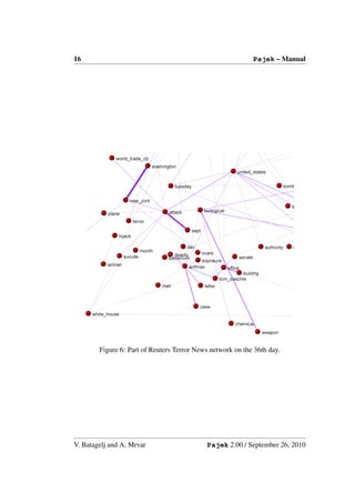
24 Pajek– Manual

Figure 8: Bow-tie – Graph structure in the web [26]

Minimal number of vertices in components can be selected. Addition-
ally, partition containing articulation points is produced: number of
biconnected components to which each vertex belongs is given. Par-
tition containing vertices belonging to exactly one bicomponent, ver-
tices outside bicomponents and articulation points is also produced:
vertices outside bicomponents get class zero, each bicomponent is
numbered consecutively (from 1 to number of bicomponents) and ar-
ticulation points get class number 9999998.

• Hierarchical Decomposition

– Clustering* – Hierarchical clustering procedure. Input is dissimilar-
ity network (matrix), which can be obtained using
Operations/Dissimilarity/Network based or read from input ﬁle.
∗ Run – Hierarchical clustering procedure. Result is hierarchy with
nested clusters and dendrogram in EPS.
∗ Options – Select method for hierarchical clustering procedure
(general, minimum, maximum, average, ward, squared ward).
– Symmetric-Acyclic – Symmetric-Acyclic decomposition of network.
Result is hierarchy with nested clusters [33].


Pajek– Manual 25

– Clustering with Relational Constraint – Hierarchical clustering with
relational constraint procedure. See:
Ferligoj A., Batagelj V. (1983): Some types of clustering with rela-
tional constraints. Psychometrika, 48(4), 541-552.
Only dissimilarities among vertices that are linked are taken into ac-
count what enables to find clusterings very fast also for large networks.
Input is network with dissimilarities, which can be obtained using
Operations/Dissimilarity/Network or Vector based or read from input
file.
∗ Run – Results are: a partition representing tree: fathers of nodes;
and two vectors: describing heights of nodes and number of ver-
tices in subtree respectivelly. If network has n vertices then ob-
tained partitions and vectors have dimension 2*n-1. Note that
this objects are not compatible with original network, you must
use Make Partition to get compatible results.
∗ Make Partition – From obtained partition representing tree gen-
erate partition compatible with original network
· using Threshold determined by Vector – From obtained
partition representing tree and one of the two vectors (all have
dimension 2*n-1) generate partition compatible with original
network by giving threshold value.
· with selected Size of Clusters – From obtained partition rep-
resenting tree and given number of vertices in clusters gener-
ate partition compatible with original network.
∗ Extract Subtree as Hierarchy – Extract subtree from obtained
Partition by giving the root as Pajek Hierarchy.
∗ Options – Select method for hierarchical clustering with rela-
tional constraint (minimum, maximum, or average) and strategy
(strict, leader, or tolerant).
• Numbering
– Depth First – Depth first numbering of selected network...
∗ Strong ... taking directions of arcs into account.
∗ Weak ... forget directions (or undirected network).
– Breadth First – Breadth first numbering of selected network...
∗ Strong ... taking directions of arcs into account.
∗ Weak ... forget directions (or undirected network).
– Reverse Cuthill-McKee – RCM numbering. See paper.


26 Pajek– Manual

– Core + Degree – Numbering in decreasing order according to all core
partition. Within the same core number vertices are ordered in de-
creasing order according to number of neighbors which have the same
or higher core number.
• Citation Weights – If a network represents citation network, weights of
lines (citations) and vertices (articles) can be computed. Results are:
– Network with values on lines representing importance of citations.
– Binary partition with vertices on the main path.
– Network containing only main path.
– Vector with importance of vertices (articles).
Different methods of assigning weights [43]:
– Search Path Count (SPC) – method. Compute from Source to Sink.
– Search Path Link Count (SPLC) – method. Each vertex is consid-
ered as Source.
– Search Path Node Pair (SPNP) – method.
Weights can also be normalized (using ﬂow or maximum value) or logged.
• k-neighbors – Select all vertices
– Input ...from which we can reach selected vertex in at most k-steps.
– Output ...that can be reached from selected vertex in at most k-steps.
– All ...Input + Output (forget direction of lines)
Result is partition where vertices are in class numbers equal to the dis-
tance from given vertex, vertices that cannot be reached from selected
vertex are in class number 9999998. After you have a partition you
can extract subnetwork.

– From Clusters – Compute selected distances according to each vertex
in Cluster. Results consist of so many partitions as is the number of
vertices in cluster. Instead of storing results in partitions they can be
stored in vectors as well.

• Paths between 2 vertices
– One Shortest – Find the shortest path between two vertices. Result
is new network. Values on lines can be taken into account (if they
present distances between vertices) or not (graph theoretical distance).
The latter possibility is faster.


Pajek– Manual 27

– All Shortest – Find all shortest paths between two vertices. Result
is new network. Values on lines can be taken into account (if they
present distances between vertices) or not (graph theoretical distance).
The latter possibility is faster.
– Walks with Limited Length – Find all walks between two vertices
with limited maximum length.
– Diameter – Find diameter – the length of the longest shortest path in
network and corresponding two vertices. Full search is performed, so
the operation may be slow for very large networks (number of vertices
larger than 2000).
– Geodesics Matrices* – Compute the shortest path length matrix and
the geodesics count matrix (for small networks only!).
– Distribution of Distances – Compute distribution of lengths of the
shortest paths and average path length among all reachable pairs of
vertices in network.
∗ From All Vertices – Take all vertices as starting points.
∗ From Vertices in Cluster – Only distances from vertices selected
by Cluster are computed.
• Critical Path Method (CPM) – Find the critical path in acyclic network –
result is new network containing the critical path. Algorithm can be used
in the area of project planning but also for analysing acyclic graphs. Addi-
tional networks containing total and free delay times of activities are gener-
ated. Two vectors (partitions) are generated, too: First containing the earli-
est possible times of coming into given states and the second containing the
latest feasible times of coming into given states.

• Maximum Flow among vertices.

– Selected Pair – Find maximum flow between selected two vertices
(algorithm looks for paths to be saturated and among them it always
selects the shortest path). Algorithm can be used in the technical area
(actual flow, values on lines mean capacities) or for analysing graphs
(if all values are 1). Result is a new network, containing the two ver-
tices and lines contributing to maximum flow between them.
– Pairs in Cluster – Find maximum flow among vertices determined by
cluster. Result is a new network, where a value on line means max-
imum flow between corresponding two vertices. Algorithm is slow:
Use it on smaller networks or clusters with limited number of vertices
only!


28 Pajek– Manual

• Vector – Get vector from network
– Centrality – Result is a vector containing selected centrality measure
of each vertex and centralisation index of the whole network [63, p.
169-219].
∗ Closeness centrality (Sabidussi).
1. Input – centrality of each vertex according to distances of
other vertices to selected vertex.
2. Output – centrality of each vertex according to distances of
selected vertex to all other vertices.
3. All – forget direction of lines – consider network as undi-
rected.
∗ Betweenness centrality (Freeman).
– Get Loops – store values of loops to vector.
– Get Coordinate – x, y, or z coordinate of network. You can also get
all coordinates at once - possibility to have more than 3 coordinates,
coordinates must contain character . (dot).
– Important Vertices – Find important vertices in directed network
(e.g. web pages, scientific citations) or 2-mode network. Result are
vectors with weights and partition with selected number of important
vertices.
∗ 1-Mode: Hubs-Authorities – In directed networks we can usu-
ally identify two types of important vertices: hubs and authorities
[46]. A vertex is a good hub, if it points to many good authorities,
and it is a good authority, if it is pointed to by many good hubs. In
obtained partition value 1 means, that the vertex is a good author-
ity, value 2 means, that the vertex is a good authority and a good
hub, and value 3 means, that the vertex is a good hub.
∗ 2-Mode: Important Vertices – Generalization of algorithm for
2-mode networks – find important vertices from first and second
subset.
– Structural Holes – Burt’s measure of constraint (structural holes) [27,
page 54-55]. Results are:
∗ network pij : the proportion of the value of i’s relation(s) with j
compared to the total value of all relations of i. where aij is the
value of the line from i to j
aij + aji
pij =
k (aik + aki )


Pajek– Manual 29

∗ network containing dyadic constraint cij – the constraint of absent
primary holes around j on i: Explanation: Contact j constrains
your i’s entrepreneurial opportunities to the extent that:
(a) you’ve made a large investment of time and energy to reach j,
and
(b) j is surrounded by few structural holes with which you could
negotiate to get a favorable return on the investment.

cij = (pij + pik pkj )2
k,k=i,k=j

∗ vector containing aggregate constraint Ci : Ci = j cij ,
Ci = 1 for isolated vertices.
– Clustering Coefficients – Compute different inherent tendency coef-
ficients in undirected network:

Let deg(v) denotes degree of vertex v, |E(G1 (v))| number of lines
among vertices in 1-neighborhood of vertex v, MaxDeg maximum
degree of vertex in a network, and |E(G2 (v))|, number of lines among
vertices in 1 and 2-neighborhood of vertex v.
∗ CC1 – coefficients considering only 1-neighborhood:
2|E(G1 (v))| deg(v)
CC1 (v) = CC1 (v) = CC1 (v)
deg(v) · (deg(v) − 1) MaxDeg
∗ CC2 – coefficients considering 2-neighborhood
|E(G1 (v))| deg(v)
CC2 (v) = CC2 (v) = CC2 (v)
|E(G2 (v))| MaxDeg
If deg(v) ≤ 1 all coefficients for vertex v get missing value (9999998).
Watts-Strogatz Clustering Coefficient (Transitivity) and Network Clus-
tering Coefficient are also reported.
– Summing up Values of Lines – Sum values of all incoming, outgoing
or all lines connected to selected vertex.
– Min of Values of Lines – Find minimum value of incoming, outgoing
– Max of Values of Lines – Find maximum value of incoming, outgoing
– Centers – Find centers in a graph using ’robbery’ algorithm: vertices
that have higher degrees (are stronger) than their neighbors steal from
them:


30 Pajek– Manual

cyclic transitive

Figure 9: Lines belonging to cyclic and transitive (shortcut) 3-rings

∗ at the beginning give to vertices initial strength according to their
degrees, or start with value 1
∗ when ’weak’ vertex is found, neighbors steal from it according to
their strengths, or they steal the same amount
– PCore – generalized cores.
∗ Degree – ordinary cores.
∗ Sum – taking values of lines into account (sum of values of lines
inside pcore).
∗ Max – taking values of lines into account (max of values of lines
inside pcore).

• Count - how many times each line belongs to predeﬁned rings

– 3-Rings – For each line count number of 3-rings to which the line
belongs.
∗ Undirected – for undirected networks – count undirected 3-rings.
∗ Directed – for directed networks – count cyclic, transitive, or all
3-rings, or count how many times each line is a transitive shortcut
(see Figure 9).
– 4-Rings – For each line count number of 4-rings to which the line
belongs.
∗ Undirected – for undirected networks – count undirected 4-rings.
∗ Directed – for directed networks – count cyclic, diamonds, genea-
logical, transitive, or all 4-rings, or count how many times each
line is a transitive shortcut (see Figure 10).


Pajek– Manual 31

cyclic transitive genealogical diamond

Figure 10: Types of directed 4-rings on arcs

3.3 Nets
Operations on two networks.
• Union of lines – Fuse selected networks. Result is a multiple relations
network. If you want to get union of networks, multiple lines must still
be deleted. Networks must match in dimension or: If one network has m
vertices and other n vertices and m < n then in network with n vertices first
m vertices must match with vertices in network with m vertices.
• Cross-Intersection – Intersection of selected networks. Networks must
match in dimension or: If one network has m vertices and other n ver-
tices and m < n then in network with n vertices first m vertices must match
with vertices in network with m vertices. Values of lines in intercept can be
sum, difference, product, quotient, min, or max of both values.
• Intersection – Intersection of selected networks where relation numbers are
taken into account.
• Cross-Difference – Difference of selected networks.
• Difference – Difference of selected networks where relation numbers are
taken into account.
• Union of vertices – Add the second network at the end of first network.
• Fragment (1 in 2) – Find all instances of fragment (determined by network
1) in network 2.
– Find – Execute command.
– Options Select appropriate model of fragment.
∗ Induced – there should be no additional lines between vertices
in instance of fragment to match (stronger condition) otherwise
additional lines can be present (weaker).


32 Pajek– Manual

∗ Labeled – labels must match (e.g. atoms in molecule). Labels are
determined by classes (colors) in partition - first partition and sec-
ond partition must be selected before searching for labeled frag-
ments. First partition determines ’labels’ of first network (frag-
ment), second partition determines ’labels’ of second (original)
network.
∗ Check values of lines – values of lines must match (e.g. in ge-
nealogy values represent sex: 1 – man, 2 – woman).
∗ Check relation number – relation numbers must match.
∗ Check only cluster – only fragments are searched. where first
vertex is one of the vertices in cluster.
∗ Extract subnetwork – produce additional result: extract subnet-
work containing vertices belonging to fragments and correspond-
ing lines.
· Retain all vertices after extracting – in extracted network
the same vertices as in original network are present, only lines
which do not belong to any fragment are removed.
∗ Same vertices determine one fragment at most – how frag-
ments on the same set of vertices (and different lines) are treated
if not checked: fragments with the same set of vertices are allowed
if checked: fragments with the same set of vertices are not allowed
∗ Repeating vertices in fragment allowed – same vertices can ap-
pear in fragment more than once (e.g. in cycles).
if not checked: found fragments always have the same number of
vertices as original fragment
if checked: some of found fragments can have less vertices than
original fragment

• Multiply First * Second - multiply selected 1 or 2 mode networks (that
match criteria for multiplication).

• Shrink coordinates (1 to 2) - Useful if you shrink network, draw shrunk
network separately, and then apply all coordinates to vertices in original
network (vertices in same class get the same coordinates). Replace coordi-
nates in network 2 using coordinates of shrunk network 1. Shrinking can be
determined using

– Partition or
– Hierarchy


Pajek– Manual 33

Michael/Zrieva/ Junius/Georgio/ Nicola/Ragnina/ Marinus/Zrieva/
Francischa/Georgio/ Anucla/Zrieva/ Nicoleta/Zrieva/ Maria/Ragnina/

Junius/Zrieva/ Lorenzo/Ragnina/
Damianus/Georgio/ Margarita/Bona/
Legnussa/Babalio/ Slavussa/Mence/

Nicolinus/Gondola/
Franussa/Bona/ Sarachin/Bona/
Nicoletta/Gondola/

Marin/Gondola/ Marinus/Bona/
Magdalena/Grede/ Phylippa/Mence/

Figure 11: Fragments – Marriages among relatives in Ragusa

3.4 Operations
One network and something else is needed as input.

• Shrink Network - Before starting shrinking, select appropriate blockmodel
in Options menu. Default is just number of lines between shrunk vertices
that must be present in original network, to cause a line in a new network.

– Partition – Shrink network according to selected partition. Vertices in
class 0 are (by default) left unchanged, others are shrunk. Results are
shrunken network and shrunken partition.
– Hierarchy – Shrink network according to selected hierarchy. Nodes
in hierarchy that are Closed are shrunk to new vertex. Cut nodes are
shrunk to virtual vertex. Border nodes are not shrunk, but they are not
visible. Vertices belonging to other nodes are left unchanged. Type of
shrinking (blockmodel) can be selected in Options menu.

• Extract from Network

– Partition – Extract sub-network according to selected partition (ex-
tract range of classes from partition). Extracted partition is produced
as additional result.
– Cluster – Extract sub-network according to selected cluster.


34 Pajek– Manual

– 2-Mode Network – Extract 2-mode network from 1-mode network:
first and second mode are determined by given set of clusters in parti-
tion.
– to GEDCOM – Extract sub-genealogy according to selected parti-
tion (weakly connected component) to new GEDCOM file (genealogy
must be read as Ore graph).

• Brokerage Roles - For each vertex j count five brokerage roles (coordi-
nator, itinerant broker, representative, gatekeeper and liaison) according to
given partition.
j j j j j

i k i k i k i k i k

coordinator itinerant broker representative gatekeeper liaison

• Dissimilarity*

– Network based – Compute selected dissimilarity matrix (d1 , d2 , d3 or
d4 ) among vertices in cluster according to number of common neigh-
bors. Corrected Euclidean-like d5 and Manhattan-like d6 dissimilari-
ties can be computed as well [13]. The obtained matrix can be used
further for hierarchical clustering procedure.
You can include vertex v to its own neighborhood or not and display
in report window only upper triangle / undirected or complete matrix
/directed (if number of vertices is low).

Nv is a set of input, output or all neighbors of vertex v; + stands for
symmetric sum, ∪ stands for set union and stands for set difference;
| stands for set cardinality; 1st maxdegree and 2nd maxdegree are the
largest degree and the second largest degree in network, respectively.

|Nu + Nv |
d1 (u, v) =
1st maxdegree + 2nd maxdegree
|Nu + Nv |
d2 (u, v) =
|Nu ∪ Nv |
|Nu + Nv |
d3 (u, v) =
|Nu | + |Nv |


Pajek– Manual 35

max(|Nu Nv |, |Nv Nu |)
d4 (u, v) =
max(|Nu |, |Nv |)
n
d5 (u, v) = ((qus − qvs )2 + (qsu − qsv )2 ) + p · ((quu − qvv )2 + (quv − qvu )2 )
s=1
s=u,v

n
d6 (u, v) = (|qus − qvs | + |qsu − qsv |) + p · (|quu − qvv | + |quv − qvu |)
s=1
s=u,v

Dissimilarities d5 and d6 are based on some matrix Q = [quv ] on ver-
tices – for example on adjacency matrix or on distance matrix. The
parameter p is usually set to value 1 or 2. In the case Nu = Nv = 0
we set all dissimilarities d1 - d4 to 1.
If Among all linked Vertices only is checked dissimilarities are com-
puted as line values of given network.
– Vector based – Euclidean, Manhattan, Canberra, or (1-Cosine)/2
dissimilarities among Vectors determined by Cluster are computed as
line values of given network.

• Vector – Operations on network and vector.
– Network * Vector – Ordinary multiplication of matrix (network) by
vector. Result is a new vector.
– Vector # Network – Result is a new network:
∗ Input – Multiplying incoming arcs in network by corresponding
vector values - multiplying i-th column of matrix by i-th compo-
nent of vector.
∗ Output – Multiplying outgoing arcs in network by corresponding
vector values - multiplying i-th row of matrix by i-th component
of vector.
– Harmonic Function – See Bollobas [25, page 328].
Let (G, a) be a connected weighted graph, with weight function a(x, y),
and let S is subset of vertices V (G). A function f : V (G) → IR is
said to be harmonic on (G, a), with boundary S, if
1
f (x) = (a(x, y)f (y)), ∀x ∈ V (G) S
A(x) y

A(x) = a(x, y)
y

Implementation in Pajek:


36 Pajek– Manual

∗ function f is determined by vector
∗ weight function a(x, y) is given by (valued) network
∗ subset S is determined by partition – vertices in class 1 are in
subset S (ﬁxed vertices), other vertices are in V (G) S
∗ additionally, permutation determines the order of vertices in com-
putations.
In Pajek you can compute the harmonic function once or iterativelly
- as long as difference between successive functions become small
enough. Components of vector that represents function f can be mod-
iﬁed immediately when they are computed or only at the end of each
iteration (after all components are computed). Procedure can be run
according to:
∗ Input – neighbors
∗ Output – neighbors
∗ All – neighbors
– Summing up neighbors – For each vertex compute the sum of class
numbers of its neighbors according to
– Min of neighbors – For each vertex compute the minimum class num-
ber of its neighbors according to
– Max of neighbors – For each vertex compute the maximum class
number of its neighbors according to
– Put Loops – put vector values as loops (arcs or edges) in current net-
work.
– Put Coordinate – put vector as x, y, or z coordinate, or put it as polar
radius or polar angle of vertices in network layout.
– Diffusion Partition – Compute diffusion partition according to thresh-
olds given in vector. Vertices in selected cluster are considered to
adopt in time 1.


Pajek– Manual 37

– Islands – Partition vertices to cohesive clusters according to weights
of vertices determined by a vector.
∗ Vertex Weights – Vertex island is a cluster of vertices of given
network with weighted vertices where the weights of the vertices
on the island are larger than the weights of the vertices in the
neighborhood. The weights are also called heights.
∗ Vertex Weights [Simple] – Simple vertex island is vertex island
with only one top.

• Transform – Transformations of network according to Partition, Cluster
and/or Vector.

– Remove Lines – Removing lines according to partition.
∗ Inside Clusters – Remove all lines with incident vertices in the
same (selected) cluster(s).
∗ Between Clusters – Remove all lines with incident vertices in
different clusters.
∗ Between Two Clusters
1. Arcs – Remove all arcs pointing from first to second cluster.
2. Edges – Remove all edges between the selected two clusters.
∗ Inside Clusters with value
1. lower than Vector value – Remove all lines inside clusters
(determined by a Partition) with value lower than the value
specified in a Vector.
2. higher than Vector value – Remove all lines inside clusters
(determined by a Partition) with value higher than the value
specified in a Vector.
Dimension of a Vector must be equal to the highest cluster number
in a Partition.
– Add – some elements to network
∗ Arcs from Vertex to Cluster – add arcs from selected vertex to
all vertices in Cluster.
∗ Arcs from Cluster to Vertex – add arcs from all vertices in Clus-
ter to selected vertex.
∗ Time Intervals determined by Partitions – change network to
temporal network using two partitions: first partition determines
initial time point, second determines terminal time point of each
vertex.


38 Pajek– Manual

– Direction – Convert to directed network where all arcs are pointing
from
∗ Lower->Higher class number.
∗ Higher->Lower class number.
Lines inside classes may be deleted or not.
– Vector(s) -> Line Values – Replace line values with result of selected
operation (sum, difference, multiplication, division) on vector(s) val-
ues in corresponding terminal and initial vertices.

• Reorder

– Network – Reorder vertices in network according to selected permu-
tation.
– Partition – Reorder vertices in partition according to selected permu-
tation.
– Vector – Reorder vertices in vector according to selected permutation.

• Count neighbor Colors – For selected network and partition a new parti-
tion is generated where for each vertex the frequency of vertices of selected
color in the neighborhood is given. Colors to be counted are determined
using cluster.

• Coloring

– Create New – Sequential coloring of vertices in order determined by
permutation. Result depends on selected permutation signiﬁcantly.
– Complete Old – Complete partial coloring of vertices in order deter-
mined by permutation. For example some vertices can be colored by
hand, but most of the vertices are still uncolored (in class 0). In this
way you can help program to produce better coloring.

• Balance* – Relocation algorithm for partitioning signed graphs (graphs
with positive and negative values on lines representing friends and enemies,
for example). Given partition is optimized to get as much as possible pos-
itive lines inside classes and negative lines between classes. Another algo-
rithm does not distinguish between diagonal and off-diagonal blocks: each
block can be positive, negative, or null. If number of repetitions is higher
than 1, initial partitions into given number of classes are chosen randomly
for every repetition separately. If program ﬁnds several optimal solutions,
all are reported. For more details about algorithm see Doreian and Mrvar
[32].


Pajek– Manual 39
Pajek - shadow 0.00,1.00 Sep- 5-1998 Pajek - shadow 0.00,1.00 Sep- 5-1998
World trade - alphabetic order World Trade (Snyder and Kick, 1979) - cores
afg uki
alb net
alg bel
arg lux
aus fra
aut ita
bel den
bol jap
bra usa
brm can
bul bra
bur arg
cam ire
can swi
car spa
cha por
chd wge
chi ege
col pol
con aus
cos hun
cub cze
cyp yug
cze gre
dah bul
den rum
dom usr
ecu fin
ege swe
egy nor
els irn
eth tur
fin irq
fra egy
gab leb
gha cha
gre ind
gua pak
gui aut
hai cub
hon mex
hun uru
ice nig
ind ken
ins saf
ire mor
irn sud
irq syr
isr isr
ita sau
ivo kuw
jam sri
jap tha
jor mla
ken gua
kmr hon
kod els
kor nic
kuw cos
lao pan
leb col
lib ven
liy ecu
lux per
maa chi
mat tai
mex kor
mla vnr
mli phi
mon ins
mor nze
nau mli
nep sen
net nir
nic ivo
nig upv
nir gha
nor cam
nze gab
pak maa
pan alg
par hai
per dom
phi jam
pol tri
por bol
rum par
rwa mat
saf alb
sau cyp
sen ice
sie dah
som nau
spa gui
sri lib
sud sie
swe tog
swi car
syr chd
tai con
tha zai
tog uga
tri bur
tun rwa
tur som
uga eth
uki tun
upv liy
uru jor
usa yem
usr afg
ven mon
vnd kod
vnr brm
wge nep
yem kmr
yug lao
zai vnd
dom

maa

mon

maa

dom

mon
cam

mex

som

yem

mex

cam

som

yem
wge

wge
kuw

swe

swe

kuw
brm

mor

rum

rum

mor

brm
dah
den

ege

gab
gha

gua

hon
hun

kmr

mat

nau
nep

pan

uga

den

ege

hun

gua
hon

pan

gha

gab

mat

dah
nau

uga

nep
kmr
aus

can

cha
chd

con

cub

ecu

egy

jam

ken

kod

mla

nze
pak

rwa

sau
sen

spa

sud

upv

usa

ven
vnd

yug

usa
can

spa

aus

yug

egy

cha

pak

cub

ken

sud

sau

mla

ven
ecu

nze

sen

upv

jam

chd
con

rwa

kod

vnd
cos

cyp
cze

cze

cos

cyp
arg

bra

bur

gre

nor

par
per

por

swi

uru

bra
arg

swi

por

gre

nor

uru

per

par

bur
afg

aut

car

eth

kor

net

tha
tog

tun

usr

vnr

net

usr

aut

tha

kor
vnr

tog
car

eth
tun

afg
alb
alg

bel
bol

bul

gui
hai

ind

jap

lao
leb

nig

phi
pol

saf

syr

bel

jap

pol

bul

leb

ind

nig

saf

syr

phi

alg
hai

bol

alb

gui

lao
chi
col

els

ice

ins

ivo

lux

mli

nic

sie

uki

zai

uki

lux

els
nic

col

chi

ins

mli

ivo

ice

sie

zai
fra

tur

fra

tur
ire
irn
irq

jor

nir

ire

irn

irq

nir

jor
fin

isr
ita

sri

tai

ita

fin

isr

sri

tai
lib

lib
liy

liy
tri

tri
Figure 12: World trade. Orderings: alphabetical and determined by clustering

Option can be used for two mode signed graphs as well: input is two mode
partition. In this case algorithm tries to find as ’clear’ as possible positive,
negative, and null blocks.
If Prespecification is checked user can define a prespecified model by en-
tering letters P, N, or 0 to cells (to require positive, negative or null blocks)
or leave cells empty (in this case the block can be of any type).
By setting penalty for small null blocks to some nonzero value, we try to
get null blocks as large as possible.

• Blockmodeling* – Generalized blockmodeling of 1-mode and 2-mode net-
works [7, 35]. For details see Section 7 on page 83. Descriptions of models
are stored on MDL files. See also block types on page 49.

– Random Start – Start the optimization with random partition(s).
– Optimize Partition – Show the criterion function for selected parti-
tion and optimize it.
– Restricted Options – Show only selected part of options (sufficient
for most users) or all options.
– Short Report – Show only main results of optimization in Report
window (sufficient for most users) or detailed, long report.

• Genetic Structure – Compute genetic structure of given acyclic network
according to given partition (of minimal vertices). As result we get as many


40 Pajek– Manual

vectors as is different clusters in partition, and the dominant gene partition.

• Permutation* – Improve given permutation according to network.

– Travelling Salesman – Can be applied to dissimilarity matrix, or mod-
ified matrix representing network (fill diagonal and change 0 in the
matrix with some large numbers):
∗ Run – Run 3-OPT algorithm for solving Travelling Salesman
Problem.
∗ Options – Put selected value on diagonal, add some artificial ver-
tices, and incident lines with large values, change value 0 with
selected (large) value.
– Seriaton – Starting with network and (random) permutation improve
the permutation using seriation algorithm from Murtagh [52, page 11-
16].
∗ 1-Mode – for ordinary (1-Mode) networks
∗ 2-Mode – for 2-Mode networks
– Clumping – Starting with network and (random) permutation improve
the permutation using clumping algorithm from Murtagh [52, page 11-
16].
∗ 1-Mode – for ordinary (1-Mode) networks
∗ 2-Mode – for 2-Mode networks
– R-Enumeration – Starting with network and (random) permutation
find such permutation that enumeration of neighbor vertices are as
close to each other as possible.

• Functional Composition – Let f be a partition or a permutation and g a
partition, a permutation, or a vector. The result is new partition, permutation
or vector r defined in the following way: r[v] = (f ∗ g)[v] = g[f [v]].

• Expand Partition

– Greedy Partition – Put vertices with unknown class number (0) in the
same class as selected vertices in partition if
∗ Input ...we can reach selected vertices in at most k-steps.
∗ Output ...we can come to vertices from selected vertices in at
most k-steps.
∗ All ...Input + Output (forget direction of lines)
Classes are joined if one vertex should belong to more classes.


Pajek– Manual 41

E5

E4 .
C4

. . C5
. M4 M5

C3 . M1 . E1

. M3
.
M2
.
.
C1
E3
C2

E2

Figure 13: Petri net

– Inﬂuence Partition – Put every vertex with unknown class number (0)
in given partition in the same class as is the class of the closest vertex.
If several vertices with known class number have the same distance,
the highest value is used.
– Make Multiple Relations Network – Transform network to a mul-
tiple relation network using a partition: if both endvertices of a line
belong to the same class in partition the multiple relations tag will be
equal to the class number of endvertices, otherwise it will be 0.

• Expand Reduction – Restore original network from reduced network (hier-
archical reduction!) and appropriate hierarchy (result is always undirected
network).

• Identify – Identify (reorder and/or join some units).

• Petri – Execute Petri net according to starting marking of places determined
by partition. Number of places in network is equal to dimension of partition.


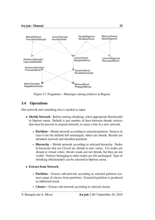
42 Pajek– Manual

Places must be defined first (1..m) then transitions (m + 1..n). What to do
if more than one transition can fire? Two possibilities:
– Random – Transition is chosen randomly.
– Complete – Complete tree of all possible transitions is built - result is
hierarchy. You can choose the maximum depth of the tree, or execute
Petri net as long as possible.
Try for example petri2 from the book of Peterson [55, page 21] or petri52
(see Figure 13) data.
• Refine Partition Refine partition according to selected network (reachabil-
ity).
– Strong ... for directed network.
– Weak ... for undirected network.
• Leader Partition – find clusters of vertices of network inside layers.

3.5 Partition
Only Partition is needed as input.
• Create Constant Partition – Create constant partition of selected dimen-
sion. Default dimension is the size of selected network (if there is one in
memory).
• Create Random Partition – Create random one or two mode partition.
• Binarize – Make binary (0-1) partition from selected partition.
• Fuse Clusters – Fuse selected cluster numbers to a new cluster.
• Canonical Partition – Transform partition to its canonical (unique) form
(vertex 1 is always in class 1, the next vertex with smallest number that is
not in the same class as vertex 1 is in class 2...).
• Canonical Partition [Decreasing frequencies] – Transform partition to its
canonical (unique) form (in class 1 the old class with the highest frequency
will be set, in class 2 the old class with the second highest frequency. . . ).
• Make Network – Generate network from partition.
– Random Network – Generate random network where degrees of ver-
tices are determined using partition.


Pajek– Manual 43

∗ Undirected – partition gives degrees of vertices in undirected net-
work.
∗ Input – partition gives input degrees of vertices.
∗ Output – partition gives output degrees of vertices.
– 2-Mode Network – Generate 2-mode network: first set consists of
vertices (v1 . . . vn ), second set consists of clusters (c0 . . . cm ). If vertex
i is in cluster j the line from vi to cj is generated. If option Existing
Clusters only is selected only clusters containing at least one vertex
are generated as vertices in the second set.
• Make Permutation – Make permutation from selected partition. (first all
vertices with the lowest class number, ...)
• Make Cluster – Transform partition to cluster.
• Make Hierarchy – Transform partition to hierarchy (nested or not).
• Make Vector – Transform partition to vector (V [i] := C[i]).
• Count, Min-Max Vector – info about cluster frequencies and minimum
and maximum vector value according to given partition.

3.6 Partitions
Operations on two partitions. Two partitions must be selected before performing
operations.
• Extract second from first – Extract from first partition vertices that satisfy
criterion (are on specified interval) determined by second partition. This
operation is useful when we have partition that actually saves some infor-
mation about vertices (for example gender). When you get (extract) some
smaller part of the network (for example vertices that are on distances less
than 3 from selected vertex), information about gender would be lost with-
out performing the same operation (extraction) on partition.
• Add Partitions – Add two partitions (useful for example when combining
Input and Output neighbors in acyclic networks).
• Min (C1, C2) – Minimum of two partitions.
• Max (C1, C2) – Maximum of two partitions.
• Fuse Partitions – Fuse two partitions – add second to the end of the first
(useful for 2-mode networks).


44 Pajek– Manual

• Expand – Expand partition to higher (original) dimension.
– First according to Second (Shrink) – Expand first partition accord-
ing to shrinking determined by second partition.
– Insert First into Second according to Third (Extract) – The current
partition was obtained by extracting selected classes defined by the
second partition from the first partition. This sub-partition was mod-
ified. Using this operation we can insert this modified sub-partition
back to the first partition.
• Intersection – of selected partitions.
• Cover with – Let p be a partition, b a binary partition, and c selected cluster
number. Result is new partition q determined in the following way:
if b(v) = 0 then q(v) = p(v) else q(v) = c.
• Merge – Let p and q be partitions and b a binary partition. Result is new
partition s determined in the following way:
if b(v) = 0 then s(v) = p(v) else s(v) = q(v).
• Make Random Network – generate random network with input degrees
determined by the first and output degrees by the second partition.
• Info – Bivariate statistical measures between selected partitions:
– Cramer’s V, Rajski – Report contingency table, compute Cramer’s V
and Rajski coefficients.
– Spearman Rank correlation coefficient.

3.7 Vector
Operations using vector.
• Create Constant Vector – Create constant vector (vector with all values
equal to selected value) of selected dimension. Default dimension is the
size of selected network (if there is one in memory).
• Extract Subvector – Extract subvector from given vector - criterion is class
in the selected partition.
• Shrink Vector – Shrink vector values according to clusters of partition to
new vector – adjusting vector to shrunken network. When shrinking several
values to one value, sum of values, mean, min, max or median value can be
used.


Pajek– Manual 45

• Make Partition – Convert vector to partition:

– by Intervals – according to selected dividing numbers in vector ver-
tices get appropriate class numbers. Intervals can be given by:
∗ First Threshold and Step – Select ﬁrst threshold and step in
which to increase threshold.
∗ Selected Thresholds – Select all thresholds or number of classes
(#) in advance.
– by Truncating (Abs) – partition is absolute and truncated vector.

• Make Permutation – Convert vector to permutation - sorting permutation.

• Make 2-Mode Network – Convert vector to 2-mode network (row or col).

• Transform – Transformations of given vector:

– Multiply by a constant.
– Add Constant to vector values.
– Absolute values of its elements.
– Absolute + Sqrt – square root of its absolute components.
– Truncate – truncated vector.
– Exp – exponential of vector.
– Ln – natural logarithm of vector.
– Power – selected power of vector.
– Normalize
∗ Sum – normalize so that the sum of elements is 1.
∗ Max – normalize so that the maximum element will have value 1.
∗ Standardize – normalize so that arithmetic mean will be 0 and
standard deviation 1.
– Invert – inverse values of vector (exception is that 0 stays 0).

3.8 Vectors
Operations on two vectors. Two vectors must be selected before performing oper-
ations.
• Add Vectors – sum of selected vectors.

• Subtract Second from First – difference of selected vectors.


46 Pajek– Manual

• Multiply Vectors – product of selected vectors.

• Divide First by Second – division of selected vectors.

• Linear Regression – fit the two vectors using linear regression. Results are:
regression line, linear estimates of second vector and corresponding errors.

• Min (V1, V2) – smaller elements in selected vectors.

• Max (V1, V2) – bigger elements in selected vectors.

• Fuse Vectors – fusion of vectors.

• Transform – two vectors to another two vectors:

– Cartesian → Polar – First vector must contain x-coordinates second
y-coordinates. Results are: vector containing polar radius and vector
containing polar angles in degrees.
– Polar → Cartesian – First vector must contain polar radius second
polar angles in degrees. Results are: vector containing x-coordinates
and vector containing y-coordinates.

Results can be (de)normalized to enable direct use in Draw window.

• Info – Pearson correlation coefficient between selected vectors.

3.9 Permutation
Only permutation is needed as input.

• Identity – Create identity permutation of selected dimension. Default di-
mension is the size of selected network (if there is one in memory).

• Random – Create random permutation of selected dimension. Default di-
mension is the size of selected network (if there is one in memory).

• Random 2-Mode – Create random permutation of selected dimension and
number of vertices in the first subset of 2-mode network. Default dimension
is the size of selected network and number of vertices in the first subset (if
there is network and corresponding partition in memory).

• Inverse – Create inverse permutation of selected permutation.

• Mirror – Create mirroring permutation of selected permutation (sort in op-
posite direction).


Pajek– Manual 47

• Make Partition – Create partition into selected number of clusters from
given permutation.

• Make Vector – Transform permutation to vector.

3.10 Permutations
Operation on two permutations.

• Fuse Permuations – Fuse two permutations – add second to the end of the
ﬁrst (useful for 2-mode networks).

3.11 Cluster
Only cluster (and partition) is needed as input.

• Create Empty Cluster – Create cluster without vertices.

• Create Complete Cluster – Create cluster with values 1..n.

• Make Partition – Transform cluster to partition.

• Binarize Partition – Binarize partition according to cluster - make binary
partition of the same dimension as the given partition, vertices that are in
cluster numbers determined by the cluster will go to class 1 other to class 0.
This allows noncontiguous ranges to be selected (other choices in Pajek
need contiguous ranges). Note the exception: In this case cluster represents
set of cluster numbers and not set of vertices numbers.

3.12 Hierarchy
Only hierarchy is needed as input.

• Extract Cluster – Extract cluster from hierarchy - the cluster is whole sub-
tree of selected node in hierarchy.

• Make Network – Converts hierarchy to network (use it for example to draw
hierarchy – drawing by layers). Closed nodes are also taken into account.

• Make Partition – Converts hierarchy to partition (according to closed nodes).

• Make Permutation – Converts hierarchy to permutation.


48 Pajek– Manual

3.13 Options
• Read - Write
– Threshold – Value of line must be higher (absolutely) than the given
threshold to generate line between two vertices.
– Max. vertices to draw – Maximum number of vertices in network to
allow drawing (to prevent long waiting).
– Large Network (Vertices) – Select the threshold number of vertices
that defines very large network. For such networks Pajek (for some
operations), asks if the old network can be destroyed and replaced by
the network that is obtained as a result. In this way we can spare a lot
of memory.
– Read - Save vertices labels? – Read / Save also labels, coordinates,
and other descriptions of vertices or not. If vertices labels are not read
(recommended if network is very large and vertices labels are long)
they can be imported later from input file using
Net/Transform/Add/Vertex Labels from File.
– Save coordinates of vertices? – Save coordinates of vertices to net-
work file (or not).
– Save complete vertex description? – When saving network to out-
put file for each vertex complete description will be written, even if
consequent vertices have the same descriptions (e.g. shapes, time in-
tervals...).
– Check equality of vertex descriptions by reading? – Enables users
to speed up reading large network files according to descriptions of
vertices: Check this option to save space when exactly the same de-
scriptions of vertices are repeated often (e.g. shapes of vertices). Un-
check this option to save time when there are several different desctrip-
tions of vertices in input file (e.g. time stamps in temporal networks).
– Check equality of line descriptions by reading? – Enables users to
speed up reading large network files according to descriptions of lines:
Check this option to save space when exactly the same descriptions of
lines are repeated often (e.g. line pattern Dots/Solid). Uncheck this
option to save time when there are several different desctriptions of
lines in input file (e.g. time stamps in temporal networks).
– Auto Report? – Automatically report all text results to file rep1.rep.
– Ore: Different relations for male and female links – When reading
genealogy as Ore graph generate 2 different types of arcs: arc with re-
lation number 1 (also value 1) represents (god)father to child relation,


Pajek– Manual 49

arc with with relation number 2 (also value 2) represents (god)mother
to child relation.
– Ore: Generate Godparent relation – When reading genealogy as
Ore graph generate also godparent relation (relation number 4) or god-
father (relation number 4) and godmother (relation number 5) rela-
tions.
– GEDCOM – Pgraph – Use pgraph format (nodes are couples or indi-
viduals) when reading genealogies (D. R. White), otherwise nodes are
only individuals.
– Bipartite Pgraph – Generate bipartite pgraph that has squares for
marriages, triangles and circles for individuals.
– Pgraph+labels – Attach also labels of lines to pgraph, when reading
GEDCOM file.
– x / 0 = Specify the result when dividing nonzero value with 0.
– 0 / 0 = Specify the result when dividing 0 with 0.
– Ignore Missing Values in Info/Vector? – When computing descrip-
tive statistics on Vector treat missing values (values larger that 9999997)
as valid numbers.
– Save Files as Unicode UTF8 with BOM? – Instead of saving to
ASCII files save files as Unicode UTF8 files.

• Select Font

– Select Proportional Font – Select proportional font for displaying
Unicode characters (e.g. in Draw window).
– Select Monospaced Font – Select non-proportional font for display-
ing Unicode characters (e.g. in Report window).
– Default Fonts – Use MS Sans Serif for proportional, and Courier New
for monospaced font.

• Blockmodel – Select type of blockmodel for shrinking. Possibilities are:

– 0..Min Number of Links
– 1..Null
– 2..Complete
– 3..Row-Dominant
– 4..Col-Dominant


50 Pajek– Manual

Figure 14: Generalized block types


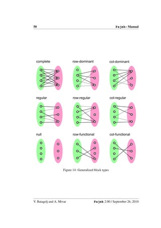
Pajek– Manual 51

– 5..Row-Regular
– 6..Col-Regular
– 7..Regular
– 8..Row-Functional
– 9..Col-Functional
– 10..Degree Density

Look in Batagelj [7] and Doreian, Batagelj, Ferligoj [35].

• Ini File

– Load – Use selected configuration of Pajek which is stored in the
file (*.ini).
– Save – Save the current configuration of Pajek into a file (*.ini).

• Use Old Style Dialogs – If Windows 7 have problems with opening/saving
files check this option.

3.14 Info
• Network – Information about network

– General – General information about network
∗ number of vertices
∗ number of arcs, edges and loops
∗ density of lines
∗ average degree
∗ sort lines according to their values (ascending or descending) to
find the most/least important lines.
– Line Values – Frequency distribution of line values.
– Indices – Different indices on network (chemical and genealogical).
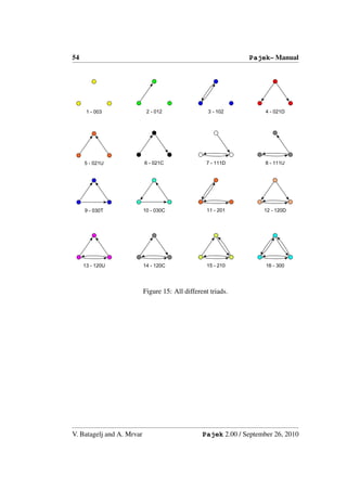
– Triadic Census – Number of different triads in network. See book of
Faust and Wasserman [63] and Figure 15 on page 54.
– Multiple Relations – General information about multiple relations
network
∗ number of relations
∗ number of arcs, edges and total number of lines for each relation


52 Pajek– Manual

– Vertex Label -> Vertex Number – Find vertex number by giving
(part of) its label, or find vertex label for given vertex number.
• Partition – General information about partition. Sort vertices according
to their class numbers (ascending or descending) to see the most important
vertices. Frequency distribution of class numbers. Average, median and
standard deviation of class numbers are also given.
• Hierarchy – General information about hierarchy. Operation is possible
only if node numbers are integers. It returns number of vertices in nodes of
hierarchy (on first level).
• Vector – General information about vector: Vertices sorted according to
their values, average, median, standard deviation and frequency distribution
of vector values into given number of classes (# – number of classes or
selected dividing values can be given).
• Memory – Available memory. Not very accurate.
• About – Information about Pajek version, authors, copyrights. . .

3.15 Tools
• R
– Send to R – Call statistical package R [56] with one vector/network,
vectors/networks selected by cluster or all currently available vectors
and/or networks.
– Locate R – locate position of statistical program R (Rgui.exe or Rterm.exe)
on the disk.
• SPSS
– Send to SPSS – Call statistical package SPSS with one partition, vec-
tor or network, partitions/vectors selected by cluster or all currently
available partitions and vectors.
– Locate SPSS – locate position of statistical program SPSS (runsyntx.exe)
on the disk.
• Web Browser – Select which web browser to open when clicking on vertex
with Shift and Right mouse button.
• Add Program – add new executable program with specified parameters to
the tools menu.


Pajek– Manual 53

• Edit Parameters – edit parameters of selected external program.

• Remove Program – remove selected external program from the tools menu.


54 Pajek– Manual

1 - 003 2 - 012 3 - 102 4 - 021D

5 - 021U 6 - 021C 7 - 111D 8 - 111U

9 - 030T 10 - 030C 11 - 201 12 - 120D

13 - 120U 14 - 120C 15 - 210 16 - 300

Figure 15: All different triads.


Pajek– Draw window 55

4 Draw Window Tools
4.1 Main Window Draw Tool
• Draw - Draw Network. A new window is open, where a new menu appears.
You can edit network by hand (move vertices using left mouse button), se-
lect a part of the picture (using right mouse button and select the area), edit
lines that belong to selected vertex by clicking on vertex using right mouse
button, spin picture using keys X, Y, Z, S, x, y, z, s. Description of Draw
window menu:

• Draw-Partition – Similar to Draw. Colors of vertices represent the classes
in selected partition. Additionally you can put selected vertex or selected
vertices into given class in partition (classes are shown using different col-
ors) by clicking on middle mouse button (or Shift+left button) (increment
class), or together with Alt (or Alt+left button) - decrement class number.
In Figure 20 on page 89 you can see which color represents selected class.
Some additional menu items that were already described appeared (you can
draw network according to layers from partition and optimise energy using
fixed vertices determined using partition). It is also possible to move the
selected class (by clicking close to vertex from that partition).

• Draw-Vector – Sizes of vertices are determined using selected vector.

• Draw-2Vectors – Sizes of vertices are determined using selected two vec-
tors (first for width second for height).

• Draw-Partition-Vector – Colors of vertices are determined using selected
partition, sizes of vertices are determined using selected vector.

• Draw-Partition-2Vectors – Colors of vertices are determined using se-
lected partition, sizes of vertices are determined using selected two vectors
(first for width second for height).

• Draw-SelectAll – Create null partition and draw network using it.

4.2 Layout
Generate layout of the network.

• Circular – Position vertices on circle

1. Original – in order determined by the network.


56 Pajek– Draw window

2. using Permutation – in order determined by current permutation.
3. using Partition – create separate circles for clusters in selected par-
tition. Center of the circle is determined by the arithmetic mean of
positions of vertices in the cluster.
4. Random – in random order.
• Energy – Automatic layout generation.
1. Kamada-Kawai – algorithm for automatic layout generation in the
plane.
(a) Free – Every position in the plane is possible.
(b) Separate Components – Optimize each component separatelly
and tile components at the end.
(c) Fix first and last – First and last vertex are fixed in opposite cor-
ners.
(d) Fix one vertex in the middle - Select vertex which will be fixed
in the middle of the picture.
(e) Selected group only – Only selected part of the picture is taking
into account during optimisation.
(f) Fix selected vertices - Selected vertices (from partition) are fixed
on given positions). This item is visible only if Draw partition is
active.
2. Fruchterman Reingold – another algorithm for automatic layout
generation (faster than Kamada-Kawai).
(a) 2D – optimisation in plane.
(b) 3D – optimisation in space.
(c) Factor – Input factor for optimal distance among vertices when
using Fruchterman Reingold optimisation.
3. Starting positions – for energy drawing (random, circular, given po-
sitions on plane xy, given z coordinates).
• EigenValues – Drawing using eigenvalues/eigenvectors (Lanczos algorithm).
Values of lines can be taken into account or not.

1. 1 1 1 – Select 2 or 3 eigenvalues and algorithm will compute cor-
responding eigenvectors. Eigenvalues may be multiple so there are
many possibilities. Some examples
(a) 1 1 1 – compute 3 eigenvectors that correspond to the first eigen-
value



Figure 16: VRML display of layout determined by eigenvectors

(b) 1 1 2 – compute 2 eigenvectors that correspond to the first eigen-
value and 1 that correspond to the second
(c) 1 2 2 – compute 1 eigenvector that correspond to the first eigen-
value and 2 that correspond to the second
(d) 1 2 3 – compute 1 eigenvector that correspond to the first, 1
that correspond to the second and 1 that correspond to the third
eigenvalue
(e) 1 1 – compute 2 eigenvectors that correspond to the first eigen-
value (2D picture)

• Tile Components – Tile weakly connected components in a plane.

4.3 Layers
Visible only if Draw partition is active. Draw in layers according to partition.
• Type of Layout – Select type of picture (2D – layers in y direction, or 3D
– layers in z direction). According to that, appropriate menu appears.
• In y direction – Draw vertices in layers (y coordinate) inside layers draw
vertices centered-equidistantly (x coordinate), z coordinate is 0.5 for all ver-
tices.



• In y direction+random in x – Same as first option, only vertices are put on
layers in random order not according to vertex numbers.

• In z direction – Draw layers in z direction, live x and y coordinates as they
are.

• In z direction + random in xy – Draw layers in z direction, x and y coor-
dinates get random values

• Averaging x coordinate – Use it after vertices are put on layers in 2D.
Iterativelly compute average x-coordinate of all neighbors and normalize.
Good approximation of global picture, but vertices are put to close to each
other. Use it on all vertices or only on selected one.

• Averaging x and y coordinates – Use it after vertices are put on layers in
3D. Iterativelly compute average x and y coordinates of all neighbors and
normalize. Good approximation of global picture, but vertices are put to
close to each other. Use it on all vertices or only on selected one.

• Tile in x direction – After averaging x coordinate vertices are put to close to
each other, so using this option vertices are repositioned to minimal distance
described in resolution.

• Tile in xy plane – Same as previous, only this option is used when drawing
3D pictures.

• Optimize layers in x direction – Optimize layout in layers using minimiza-
tion of the total length of lines.

1. Forward – go from first to last layer. In the current layer optimize
only layers having numbers equal or one smaller as the current layer
number.
2. Backward – go from last to first layer. In the current layer optimize
only layers having numbers equal or one larger as the current layer
number.
3. Complete – go from first to last layer. In the current layer optimize
only layers having numbers equal or one smaller or one larger as the
current layer number.

• Optimize layers in xy plane – Same as previous, only this option is used
when drawing 3D pictures.



• Resolution – How many additional positions are available on layers. Works
only if Pgraph is selected. The higher the resolution, the better is the result
of optimization, but also slower.

4.4 GraphOnly
Show complete picture without labels and arrows.

4.5 Previous
Draw previous network, and/or partition and/or vector which are loaded in Pajek
(depending on selection in Options/PreviousNext/Apply to).

4.6 Redraw
Redraw network.

4.7 Next
Draw next network, and/or partition and/or vector which are loaded in Pajek
(depending on selection in Options/ PreviousNext/ Apply to).

4.8 ZoomOut
Zoom out (visible only when zooming in layout).

4.9 Options
Additional options for picture layout.

• Transform – Transformations of picture.

1. Fit area
(a) max(x), max(y), max(z) – Draw picture as big as possible to fit
area (resize each coordinate to fit in picture independently).
(b) max(x,y,z) – Resize to fit in area but keep real proportions (re-
size according to largest distance in all three coordinates, e.g.
molecule).
2. Resize – Resize picture (or selected part of it) in all three directions
for selected factor.



3. Translate – Translate picture (or selected part of it) in space.
4. Reflect y axis – Reflect picture (or selected part of it) around y axis.
5. Rotate 2D – Rotate picture (or selected part of it) in xy plane.
6. Fisheye – Fisheye transformation (cartesian or polar) of picture. If no
vertex is selected the middle point of picture (or selected part of it) is
used as focus, otherwise first selected vertex will be used as focus.

• Values of lines – Meaning of values of lines during energy drawing or
eigenvectors computing (no meaning, similarities, dissimilarities (distances)).

• Mark vertices using – Labels can be marked using

1. labels
2. numbers
3. partition clusters (if partition of the same size is also selected)
4. vector values (if vector of the same size is also selected)
5. without labels
6. without labels and arrows
7. cluster only – only vertices belonging to the current Cluster are labeled
in the layout.

• Lines – Select the way the lines are drawn:

1. Draw Lines
(a) Edges – draw edges or not
(b) Arcs – draw arcs or not
(c) Relations – draw all lines (leave empty string) or just lines be-
longing to selected relations, e.g. 1-3,6,10-15.
2. Mark Lines
(a) No – do not mark lines
(b) with Labels
(c) with Values
3. Different Widths – if checked, the width of the lines will be deter-
mined by their line values.
4. GreyScale – if checked, the color in grayscale of lines will be deter-
mined by their line values.



• Size – Determine size of vertices, width of vertices border, width of lines,
size of arrows, size of font or turn them to default values.
Sizes of vertices can be set to autosize (0-average). They can be read from
input file (x fact and y fact) or determined by one vector (currently selected)
or the two currently selected vectors. FontSize can be proportional to values
stored in third partition.

• Colors – Determine color of background, vertices, border of vertices, edges,
arcs and font (of vertices labels and lines labels) or turn them to default
values. Colors of edges/arcs can represent relation number of lines. You
can select which color should represent given class using Relation Colors.
You can also use colors of vertices (ic Red), border of vertices (bc Blue),
arcs and edges (c Green) as defined on input file (see Figure 19, page 88).
FontColor can be determined by values stored in second partition.
Example NET file:

*Vertices 9
1 "a" ic Pink bc Black
2 "b" ic Yellow bc Cyan
3 "c" ic Cyan bc Yellow
4 "d" ic Purple bc Orange
5 "e" ic Orange bc Brown
6 "f" ic Magenta bc Green
7 "g" ic Brown bc Magenta
8 "h" ic Red bc Blue
9 "i" ic Green bc Magenta
*Arcs
1 2 1 c Blue
2 3 1 c Red
3 4 1 c Black
4 5 1 c Yellow
5 6 1 c Gray
6 7 1 c Cyan
7 8 1 c Magenta
8 9 1 c Purple
9 1 1 c Brown

• Layout – Layout options

1. Redraw – Redraw whole network during or/and after moving of se-
lected vertex, and/or redraw if draw window is paint.
2. Real xy proportions – The draw window has always square shape or
not.
3. Arrows in the Middle – Draw arrows in the middle of lines – not at
terminal vertices.
4. Size of vertex 0 – How to handle vertices of size 0 (size of vertex is
determined in input file or using vector)?



(a) Hide vertex – vertices of size 0 are shown or not.
(b) Hide attached lines – lines with one end in vertex of size 0 are
shown or not.
5. Decimal Places – How many decimal places to use when marking
vertices using vectors.
6. Show SubLabel – Select the position of the vertices sublabel that is
shown in network layouts.
• ScrollBar On/Off – Show/Hide the scrollbars in the top left corner of Draw
window. When part of picture is selected, scrollbar is used for moving.
When whole picture is selected, scrollbar is used for spinning (like pressing
keys X, Y, Z, x, y, z – spinning around axis deﬁned by the key, and S – spin
around selected normal)
• Interrupt – Interrupt period during optimisation (stop every ? second, or
not)
• Previous/Next – Select parameters when using Previous or Next commands
for drawing sequence of networks in draw window:
1. Max. number – How many networks to show in sequence. If the
number is higher than number of existing networks the sequence will
stop earlier.
2. Seconds to wait – Seconds to wait between the two layouts.
3. Optimize Layouts – Optimize the current layout or not. If the se-
quence of networks is obtained from the same network, it is useful to
choose Energy/Starting Positions/ Given xy to start optimization with
existing coordinates.
(a) Kamada-Kawai – Optimize the current layout using
Kamada-Kawai algorithm.
(b) 2D Frucht. Rein. – Optimize the current layout using 2D Frucht.
Rein. algorithm.
(c) 3D Frucht. Rein. – Optimize the current layout using 3D Frucht.
Rein. algorithm.
(d) No – Do not optimize the layout, just show the picture.
4. Apply to – Which object (Network, Partition, Vector) will change
when Previous or Next is selected:
(a) Network – The previous / next network in memory is drawn. If
Draw-Partition is selected and the new network matches in di-
mension with selected partition, the same partition will determine



colors of vertices of the new network. If Draw-Vector is selected
and the new network matches in dimension with selected vector,
the same vector will determine sizes of vertices of the new net-
work.
Option can be used to show several networks of equal size using
the same partition/vector.
(b) Partition – The previous / next partition in memory is selected. If
Draw-Partition is selected: The same network is drawn using pre-
vious / next partition (network and partition must match in size).
Option can be used to show several partitions of selected network.
(c) Vector – The previous / next vector in memory is selected. If
Draw-Vector is selected: The same network is drawn using previ-
ous / next vector (network and vector must match in size).
Option can be used to show several vectors of selected network.
By checking several objects (Network, Partition, Vector) at the same
time previous / next networks will be drawn using previous / next parti-
tions and (or) vectors at the same time. All consequent selected objects
must match in size.

• Select all – Select all vertices in window (then possible to put vertices in
given class).

4.10 Export
Export layout of the network to one of the following two or three dimensional
formats:

• 2D – two dimensional exports:

– EPS/PS – Export to EPS format (with or without Clip, or WYSIWYG
[What You See Is What You Get – exported EPS picture is similar to
picture in Draw window – except that colors are Black/White or color
determined by partition]). PS – Export to PS format (similar to EPS
but without header).
– SVG – Export to SVG (Scalable Vector Graphics) format. Additional
controls over layout can be included in SVG or HTML. The plugin for
examining layouts can be obtained from Adobe [1].
Linear or radial gradients (continuously smooth color transitions from
one color to another) can be selected as well – up to three background
colors can be selected in Export/Options window.



1. General – Export to SVG without possibility to choose parts of
the picture.
2. Labels/Arcs/Edges – Export with possibility to turn labels, arcs
and/or edges on/off.
3. Partition – Export to SVG using one or two partitions. One parti-
tion is used by default: the same partition determines classes and
colors. But, if two partitions are defined by Partitions menu, first
partition will determine classes, the second colors of vertices.
(a) Classes – User can turn selected classes and lines among
classes on/off.
(b) Classes with semi-lines – User can turn selected classes on/off.
Lines among classes are drawn as semi-lines.
(c) Nested Classes – Upper classes are nested in lower – when-
ever selected class is turned on all higher classes are turned on
too, and all lower classes are turned off (suitable for showing
cores, for example).
4. Line Values – Export to SVG using values of lines. Threshold
values or number of classes must be given. If you input #n, n
classes of equal size will be generated. According to obtained
thresholds, subsets of lines (and incident vertices) are defined and
can be turned on/off inside web browser.
(a) Classes – User can turn lines of selected value and incident
vertices on/off.
(b) Nested classes – User can turn lines of selected value or
higher (lower) and incident vertices on (off).
(c) Options – Additional options to emphasize the values of lines
using some visual properties.
Different Colors – Subsets of lines are drawn using colors
which are used for partitioning vertices too.
Using GreyScale – The darkness of a line corresponds to its
value.
Different Widths – The width of a line corresponds to its
value.
5. Multiple Relations Network – Export multiple relations network
to SVG. User can show/hide one or more relations in the layout.
6. Current and all Subsequent – If checked the current network
and all subsequent networks will be exported to SVG. For each
network separate html file is generated. Files are given the fol-
lowing names: file001.htm, file002.htm,... Generated html files



get additional links (Previous/Next) to transition among them. If
also next partitions / vectors fit in dimension to dimension of net-
works, partitions will determine color of vertices, vectors will de-
termine sizes of vertices. Subsequent is applied to any combina-
tion of [Network, Partition, Vector] (one of the three objects only,
any pair of them or all three of them) according to selection in
Options/Previous/Next/ Apply to in Draw window.
– Bitmap – Export to Windows bitmap (bmp) format.

• 3D – three dimensional exports:

– X3D – Export to X3D (XML based 3D computer graphics, the suc-
cessor of VRML) format.
– Kinemages – Export to Kinemages format with balls or labels. You
need Mage or King viewer to watch it. A free copy of the Mage soft-
ware can be downloaded from its site [57].
1. Current Network Only – Export only current network to Kine-
mages. Two partitions defined by Partitions menu can be used -
one for generations one for colors.
2. Current and all Subsequent – Export current network and all
subsequent networks (use commands KINEMAGE/Next or Ctrl
N in Mage). If also next partitions/vectors fit in dimension to di-
mension of networks, partitions will determine color of vertices,
vectors will determine sizes of vertices. Subsequent is applied to
any combination of [Network, Partition, Vector] (one of the three
objects only, any pair of them or all three of them) according to
selection in Options/Previous/Next/ Apply to in Draw window.
3. Multiple Relations Network – Export with possibility to hide /
show selected relations.
– VRML – Export to VRML (Virtual Reality) format. For examining
it you need a VRML viewer such as Cortona [29] or (older) Cosmo
player [30].
– MDL MOL file – Export to MDL Molfile format. You need Chime
plugin (Chemscape Chime) for Netscape to explore it [50].

• Options – EPS, SVG, X3D and VRML default options (see section on Ex-
ports to EPS/SVG/X3D/VRML).
• Append to Pajek project file – Add current network to the end of selected
project file (used by program PajekToSvgAnim).



– Select file – Select project file.
– Append – Append to project file.

4.11 Spin
• Spin around – Spin network around selected normal.

• Perspective – Distant vertices are drawn smaller (or not).

• Normal – Normal vector to spin around.

• Step in degrees – Step in degrees when showing rotation.

4.12 Move
Give additional constraints on hand vertex moving:

• Fix – Fix (do not allow) moving in x or y direction, or do not allow changing
distance from center (circulating).

• Grid – Define (x, y) positions on grid, these become feasible positions for
vertices during moving by hand.

• Circle – Define (x, y) positions on concentric circles, these become feasible
positions for vertices during moving by hand.

• Grasp – Determine which additional vertices are moving when clicking
with left mouse button close to vertex in given class. Vertices that will be
moved are in the:

1. Closest Class Only
2. Closest Class and Higher
3. Closest Class and Lower

4.13 Info
– Select aesthetic properties of the current layout to compute:

• Closest Vertices

• Smallest Angle

• Shortest/Longest Line



• Number of crossings if lines

• Vertex Closest to Line

• All Properties

Remember that coordinates of vertices must be between 0 and 1!


68 Exports to EPS/SVG/X3D/VRML

5.1 Defaults
If you have no labels in Draw window when you call Export there will also be no
labels in EPS/SVG picture, otherwise numbers/labels like in Draw window will
be shown. If you are looking at the picture using Draw/Partition, the same colors
will be automatically used in EPS/SVG picture too.

5.2 Parameters in EPS, SVG, X3D, and VRML Defaults Win-
dow
Window is divided into 5 frames, two on the left and three on the right.
Note that settings you made in this window are overwritten if the parameters
are specified in Pajek input (NET) file.

Top frame on the left – EPS/SVG Vertex Default
This frame defines default drawing of vertices when we export layouts to EPS and
SVG:

• Interior Color – interior color of vertices (see Figure 19, page 88). If
drawing using Partition is used, partition colors will overwrite the specified
interior color.

• Border Color – color of the borderline of vertices.

• Label Color – color of label of vertices.

• Border Width – width of the borderline of vertices.

• Label Position: Radius /Angle – position where the label will be dis-
played:

– Radius – distance of beginning of vertex label from vertex center –
first polar parameter.
– Angle – position of vertex label in degrees - second polar parameter
(0..360).

If radius is equal to 0, the label will be centered, otherwise it will be left
aligned on the specified position.

• Fontsize – size of font of vertices labels.


Exports to EPS/SVG/X3D/VRML 69

• Label Angle – angle in which vertex labels will be displayed: if angle is
smaller than 360, it means relative according to horizontal line (0 – horizon-
tally); otherwise it is relative to center of the layout (360 – concentrically).
The latter is useful when all vertices are drawn in concentric circle(s) using
Layout/Circular.
• x/y Ratio – ratio between size of vertex in x and y direction (e.g., value 1
for circle, value larger/smaller than 1 for ellipse).
• Shape – default shape of vertex (ellipse, box, or diamond).
• Shapes file – default shapes file, double click to change it.
• Export options overwrite shapes file – if checked: options selected in this
window overwrite options defined in shapes file, otherwise default values
for each shape are defined in selected shapes file.

Bottom frame on the left – EPS/SVG Line Default
This frame defines default drawing of lines when we export layouts to EPS and
SVG:

• Edge Color – color of edges.
• Edge Width – width of edges.
• Arc Color – color of arcs.
• Arc Width – width of arcs.
• Pattern – pattern for drawing lines (Solid or Dots).
• Arrow Size – size of arrows.
• Arrow Position – distance of arrow from terminal vertex: If distance is
between 0 and 1, it means relative distance according to arc length, e.g.: 0 –
arrow touching the terminal vertex; 0.5 – arrow in the middle of the arc. If
distance is larger than 1 it means absolute distance from the terminal vertex
(this is useful if you want to have all arcs on the same distance from terminal
vertex, regardless of arcs length)
• Label Color – color of line labels.
• Label Angle – angle in which label of line will be displayed: if angle is
smaller than 360, it means relative to direction of line (0 – parallel to line);
otherwise it is relative to horizontal line (360 – horizontally).



• Label Position – position of the center of line label – position is point on
the line - distance of the center of line label from terminal vertex (see also
Arrow Position)
• Fontsize – size of font of line labels.
• Label Position: Radius /Angle – position where the center of line label
will be displayed according (relative) to Label Position:
– Radius – distance of center of line label from point defined by Label
Position - first polar parameter.
– Angle – position of label in degrees - second polar parameter (0..360).
• Only straight lines – drawing bidireced and multiple lines without curves.

Top frame on the right
This frame defines some additional defaults when we export layouts to EPS, SVG,
X3D, or VRML:
• EPS, SVG, X3D, VRML Size of Vertices – default size of vertices when
exporting to X3D/VRML (valid for EPS and SVG exports as well).
• X3D/VRML Size of Lines – width of lines in X3D/VRML.
• EPS: Use RGB colors instead of CMYK – in description of colors in EPS
file RGB is used (default is CMYK).
• SVG: 3D Effect on Vertices – if selected, gradient will be applied to get
3D look of vertices.

Middle frame on the right – Background Colors
This frame defines background color when exporting to EPS/SVG/X3D/VRML
and gradients (continuously smooth color transitions from one color to another)
when exporting layouts to SVG/X3D:
• Bckg. Color 1 – Background color for layout in EPS/SVG/X3D/VRML.
• Bckg. Color 2 – the second color for SVG/X3D export. No – means without
second color, otherwise selected gradient will be used.
• Bckg. Color 3 – the third color for SVG/X3D export – gradient.
• Gradients – type of gradient to use in SVG (No, Linear, or Radial). In X3D
only Radial gradient is supported.



Bottom frame on the right
This frame deﬁnes some additional defaults when we export layouts to EPS:

• Left, Right, Top, Bottom – additional border around layout when exporting
to EPS (only when EPS Clip format is selected)

• Border Color – color of borderline of layout. It is used for export to SVG
as well. No – means without borderline.

• Border Radius – radius of borderline of layout (if greater than 0 it means
oval instead of rectangle).

• Border Width – width of borderline of layout.

Figure 17: Spider / Kriˇevec; Photo: Stana.
z



5.3 Exporting pictures to EPS/SVG – defining parameters in
input file
Definition of Network (and its picture) on Input ASCII File
For every vertex and line we can specify in details how it should be drawn (colors,
shapes, sizes, patterns, rotations, widths...).
A kind of standardized language is used for describing networks. The follow-
ing reserved words are used:
1. *Vertices n – definition of vertices follows. n is number of vertices. Each
vertex is described using following description line:
vertex num label [x y z] [shape] [changes of default parameters]
Explanation:

• vertex num – vertex number (1, 2, 3 . . . n)
• label – if label starts with character A..Z or 0..9 first blank determines
end of the label (e.g., vertex1), labels consisting of more words must
be enclosed in pair of special characters (e.g., ”vertex 1”)
• x, y, z – coordinates of vertex (between 0 and 1)
• shape – shape of object which represents vertex. Shapes are defined
in file SHAPES.CFG (ellipse, box, diamond, triangle, cross, empty)
Description of parameters in shapes.cfg:
– SHAPE s – s is external name of vertex (used in Pajek network
file)
– sh – sh can be ellipse, box, diamond, triangle, cross, empty. This
is the name of PostScript procedure that actually draws object
(procedure is defined in drawnet.pro).
– s size – default size
– x fact – magnification in x direction
– y fact – magnification in y direction
– phi – rotation in degrees of object in + direction (0..360)
– r – parameter used for rectangle and diamond for describing ra-
dius of corners (r = 0 – rectangle, r > 0 – roundangle)
– q – parameter used for diamonds – ratio between top and middle
side of diamond (try q 0.01, q 0.5, q 2, ...)
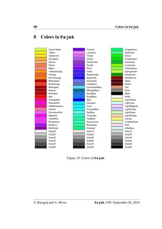
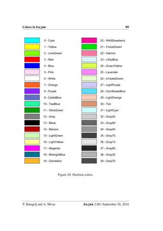
– ic – interior color of vertex. See Figure 19, page 88 for the list of
possible colors.
– bc – boundary color of vertex



– bw – boundary width of vertex
– lc – label color
– la – label angle in degrees (0..360)
– lr – distance of beginning of vertex label from vertex center (ra-
dius – first polar parameter)
– lphi – position of label in degrees (0..360) (angle phi – second
polar parameter)
– fos – font size
– font – PostScript font used for writing labels (Helvetica, Courier,
...)
– HOOKS – positions where edges can join the selected shape - ac-
cording to s size. Three different ways to specify these positions:
(a) CART – x y – positions in Cartesian coordinates (x,y)
(b) POLAR – r phi – positions in polar coordinates, phi is posi-
tive angle (0..360)
(c) CIRC – r phi1 – iteration of positions in polar coordinates r
– radius, phi = k ∗ phi1, k = 1, 2, ..; k ∗ phi1 ≤ 360

Default values can be changed for each vertex in definition line, example:
1 ”vertex one” 0.3456 0.1234 0.5 box ic White fos 20
Explanation: White box will represent vertex 1, label (vertex one) will be
displayed using font size 20.

2. *Arcs (or *Edges) – definition of arcs (edges). Format:
v1 v2 value [additional parameters]
Explanation:

• v1 – initial vertex number
• v2 – terminal vertex number
• value – value of arc from v1 to v2

These three parameters must always be present. If no other parameter is
specified, the default arc will be black, straight, solid arc with following
exceptions:

• if value is negative, dotted line will be used instead of solid,
• if arc is a loop (arc to itself) bezier loop will be drawn,
• if bidirected arc exists two curved bezier arcs will be drawn.



Arrow will be drawn at the end of the edge (at terminal vertex).
As we mentioned, hooks are used to specify exact position where line joins
vertices.
Additional parameters:

• w – width of line
• c – color of line
• p – pattern of line (Solid, Dots)
• s – size of arrow
• a – type (shape) of arrow (A or B)
• ap – position of arrow
– ap = 0 – arrow at terminal vertex
– 0 < ap ≤ 1 – proportional distance from terminal vertex (accord-
ing to line length)
– ap > 1 – absolute distance
• l – line label (e.g. ”line 1 2”)
• lp – label position (look at ap)
• lr – label radius (position of center text from point on edge )
• lphi – label radius (angle of center text according to point on edge ) (lr
and lphi are polar coordinates)
• lc – label color
• la – label angle
(0 < la < 360 – relative to edge, la ≥ 360 – absolute angle according
to x axis)
• fos – font size of label
• font – PostScript font used for writing labels (Helvetica, Courier, ...)
• h1 – hook at initial vertex (0 – center, -1 the closest, 1, 2.. user deﬁned)
• h2 – hook at terminal vertex
• a1 – angle at initial vertex (Bezier)
• k1 – velocity at initial vertex (Bezier)
• k2 – velocity at terminal vertex (Bezier)
• a2 – angle at terminal vertex (Bezier)



Special shapes of lines can be defined using combinations of alpha1, k1,
alpha2, k2:

• alpha1 = alpha2 = 0, k1 ≥ 0, k2 ≥ 0 – straight line (default)
• alpha1 = alpha2 = 0, k1 = −1, k2 > 0 – oval edge with radius k2
(measure of radius is absolute as explained above)
• alpha1 = alpha2 = 0, k1 = −1, k2 < 0 – second possible oval edge
with radius −k2
• alpha1 = alpha2 = 0, k1 = −2, k2 > 0 – circular arc with radius k2
in positive direction
• alpha1 = alpha2 = 0, k1 = −2, k2 < 0 – second possible circular
arc with radius −k2 in positive direction
• alpha1 = alpha2 = 0, k1 = −3, k2 > 0 – circular arc with radius k2
in negative direction
• alpha1 = alpha2 = 0, k1 = −3, k2 < 0 – second possible circular
arc with radius −k2 in negative direction
• alpha1 = alpha2 = 0, k1 = −4 – double edge
• alpha1 or alpha2 = 0, k1 > 0, k2 > 0 – Bezier curve (if alpha1
and alpha2 have different signs line goes from one to another side of
straight line connecting both vertices, if alpha1 and alpha2 have the
same sign – line stays on the same side of straight line connecting both
vertices)

3. *Edges – definition of edges.
The same parameters as for arcs can be used, except that type (a), size (s)
and position (ap) have no meaning for edges.

PS and EPS
• PS – Export to Postscript (.PS) without header (drawnet.pro). Use it to spare
space, if you have many pictures and your word processor enables you to
define the header separately (like in LTEX).
A

• EPS – Export into file with Encapsulated PostScript description (.EPS).
Drawnet.pro is already inserted in the beginning. The picture is complete,
you can include it into text, make it bigger or smaller (without losing qual-
ity), rotate it, print it on Postscript printer, view it with GhostScript viewer,
convert it to PDF, JPG...



An example
*Vertices 4
1 "ellipse" 0.120 0.285 0.5 ellipse x_fact 5 y_fact 3 fos 20 ic LightYellow lc Red
2 "box" 0.818 0.246 0.5 box x_fact 5 y_fact 3 fos 20 ic LightCyan lc Blue
3 "diamond" 0.368 0.779 0.5 diamond x_fact 7 y_fact 3 fos 20 ic LightGreen lc Black
4 "triangle" 0.835 0.833 0.5 triangle x_fact 9 y_fact 3 fos 20 ic LightOrange lc Brown lr 30 lphi 200
*Arcs
1 1 1 h2 0 w 3 c Blue s 2 a1 -130 k1 0.6 a2 -130 k2 0.6 ap 0.25 l "Bezier loop" lc OliveGreen fos 20 lr 13 lp 0.5 la 360
2 1 1 h2 1 a1 120 k1 1 a2 10 k2 0.8 ap 0 l "Bezier arc" lphi 270 la 180 lr 13 lp 0.5
1 2 1 h2 -1 a1 40 k1 2 a2 -30 k2 0.8 ap 0 l "Bezier arc" lphi 90 la 0 lp 0.75
4 2 -1 l "Straight dotted arc" p Dots c Red
*Edges
1 3 1 l "Straight edge" lp 0.4
3 4 1 l "Straight edge"

You have to set some options in Pajek’s draw window: for example
Options / Lines / Mark Lines / with labels
to activate the display of line labels.

c
Bezier loop er ar
Bezi

box
ellipse

Be
zi er
arc

Straight dotted arc
St
ra
igh
te
dg
e

diamond Straight edge

triangle

Figure 18: Example picture

5.4 Using Unicode in Pajek’s pictures
Sometimes we would like to use in Pajek’s picture some characters from unusual
alphabets (special symbols, Cyrillic, Greek, Arabic, Chinese, ...). They are avail-
able in Unicode. Pajek supports Unicode UTF8 ﬁles with BOM from version 2.00
on.



Some hints on using Unicode in Pajek:

• Using the free Unicode editor BabelPad we prepare the Unicode version
of the *.NET file. Use the U tool (Unicode table) to enter the Unicode
characters.

• Using the BabelPad option File/Save as/UTF8 and checking Byte
Order Mark you save network in a Unicode file.
You can use also File/Save as/ASCII plus decimal NCR. In
this way we transform Unicode file into an ASCII file in which the Uni-
code characters are represented using numeric codes &#dddd;.
Any of the two files generated can be read by Pajek and proper Unicode
characters will appear in Draw, Report and other windows provided that you
select proper proportional and monospaced font in Options/Select
Font in Pajek Main menu. We suggest to use Arial Unicode MS or
Lucida Sans Unicode (one of them usually comes with Windows) for
proportional font and GNU Unifont for monospaced font. Courier New
can be used too.
When saving networks they are stored as ASCII files by default (nonASCII
characters are stored as &#dddd;) unless you check Options/Read-Write/Save
Files as Unicode UTF8 with BOM.
The file is used in Pajek 2.00 (or higher) to produce picture. The picture is
exported in the SVG format.

ανδρει
ανδρει

⑤⑨④②⑦

⑤⑨④②⑦ Vlado
Vlado

焹焓燝牕犫獨

焹焓燝牕犫獨
गङथफञऑक
♔♕♖♗♘♙ गङथफञऑक
♔♕♖♗♘♙
∰∈∀≋∞⊚
∰∈∀≋∞⊚
‫זלגהשעצ‬
‫זלגהשעצ‬
Андреј
‫ﻛﺼﺘﺒﺨﻴﺮي‬ ‫ﻛﺼﺘﺒﺨﻴﺮي‬ Андреј
Pajek Pajek

• The SVG picture can be opened in the free drawing program InkScape.
Here we can make some additional enhancements of the picture.



• In InkScape we can, using the option File/Save as/pdf or eps, save
the picture in the desired format PDF or EPS or some other) with labels con-
taining Unicode characters. Note that the PDF (1.4 or higher) also supports
the transparency. The EPS ﬁle can be inserted in Word document.

A set of example ﬁles is available in ZIP.
Similar approach can be used also for 3D models in X3D. For their inspection
we recommend the use of Instant Player.


Using Macros in Pajek 79

6 Using Macros in Pajek
6.1 What is a Macro?
A macro enables you to record a sequence of primitive Pajek commands into a
file. You can use this file later to execute the saved sequence of commands without
selecting one by one.

6.2 How to record a Macro?
1. First load all objects (networks, partitions,...) which will be used by a
macro.

2. Select objects which will be used in macro (for example, network which
will be first used must be shown in Network ComboBox).

3. Choose Macro/Record and select the name of macro file (default extension
is .mcr).

4. Use Pajek as usual to define a sequence of commands. We advise to
add additional comments to macro file using Macro/Add Message. When
running macro this comments are displayed in Report window and help you
to follow the macro execution.

5. At the end select Macro/Record again to stop recording.

6.3 How to execute the Macro?
1. First load object(s) that will be used as input in macro execution.

2. Choose Macro/Play and select the macro file.

6.4 Example
The following macro performs topological sort of an acyclic network:

NETBEGIN 2
CLUBEGIN 1
PERBEGIN 1
CLSBEGIN 1
HIEBEGIN 1
VECBEGIN 1
NETPARAM 1



Msg Depth Partition
C 1 DEP 1 (10)
Msg Make Permutation
P 1 MPER 1 (10)
Msg Reordering network
N 2 REOR 1 1 (10)
The first seven commands store the current state of ComboBoxes. The acyclic
network on which we want to execute topological sort must be at the top of Net-
work ComboBox before starting the macro.

6.5 List of macros available in installation file
6.5.1 Macros prepared for genealogies and other acyclic networks
• Path – find shortest chain (undirected path) between the two vertices.
• Descendants – find all vertices ’later’ than selected vertex (in a p-graph).
• Ancestors – find all vertices ’before’ the selected vertex (in a p-graph).
• Cognatic3 – find vertices three generations ’before’ and three generations
’after’ the selected vertex (in a p-graph).
• Cognatic – find all reachable vertices ’before’ and all ’after’ the selected
vertex (in a p-graph).
• Layers, Layers1, Layers2 – draw acyclic network in layers (different al-
gorithms).
• zLayers – draw acyclic network in layers in z direction.
• LongestPatrilineage – find the longest patrilineage in Ore-genealogy. The
genealogy must be read with the option Ore graph: 1-Male, 2-Female
links checked.

• LongestMatrilineage – find the longest matrilineage in Ore-genealogy. The
genealogy must be read with the option Ore graph: 1-Male, 2-Female
links checked.

• NumDescendants – for each vertex compute the size of output domain
(number of descendants in Ore-graph).
• NumAncestors – for each vertex compute the size of input domain (number
of ancestors in Ore-graph).


Using Macros in Pajek 81

6.5.2 Macros prepared for computing derived kinship relations
Pajek generates three relations when reading genealogy as Ore graph with the
option Ore graph: 1-Male, 2-Female links checked:
1 : is a father of
2 : is a mother of
3 : is a spouse of
Other kinship relations can be obtained from these relations by running macros.
Gender partition is also result of reading genealogy and is input to the following
macros.

4 : is a parent of
5 : is a child of
6 : is a son of
7 : is a daughter of
8 : is a husband of
9 : is a wife of
10 : is a sibling of
11 : is a brother of
12 : is a sister of
13 : is an uncle of
14 : is an aunt of
15 : is a semisibling of

Using macro add all relations you can add all above relations at once.
As a test/example file you can use */pajek/data/family.ged

6.6 Repeating last command
Macro submenu enables to run the last command executed by Pajek several times
applied to different successive objects, as well.
Example: after loading 100 networks in Pajek, execute degree partition on
the first network and run Repeat Last Command by typing 99 to compute degree
partition on all other networks.
Commands that include several objects can be run as well (e.g. extracting sub-
networks according to selected partition(s)). There are 3 different possibilities for
extracting from the set of networks (possibilities are selected by fixing appropriate
objects):

• for all networks extracting is determined by the same partition (increment-
ing applied to network, not applied to partition – partition is fixed)



• for all networks extracting is determined by another partition (incrementing
applied to network and to partition – nothing is fixed)

• for one network several extractions are determined by different partitions
(incrementing not applied to network, applied to partition – network is
fixed)

Important: Always first execute the command on the first loaded object(s).
Repeating will start with object(s) that have object number(s) one higher than the
object(s) on which the command was executed.
If the result of the command is also a constant, all constants are stored in a
vector. In Pajek the following constants exist: number of vertices, arcs, edges,
network densities, centralization indices, diameter, relinking index, correlation
and contingency coefficients, number of fragments, main core number, number
of components, length of critical path, maximum flow, distance between vertices,
number of islands, minimum and maximum value in partition / hierarchy, mini-
mum, maximum, arithmetic mean, median and standard deviation in vector.


Blockmodeling in Pajek 83

7 Blockmodeling in Pajek
The blockmodeling option is an embedding of the programs for optimization ap-
proach to generalized blockmodeling MODEL2 and TwoMODEL from package
STRAN – STRucture ANalysis [9] into Pajek.
The blockmodeling command seeks for the best partition of a given network
satisfying given types of blocks – generalized blockmodeling [7, 35]. The block-
model can be built inside Pajek (if User Defined is selected) and/or its description
can be stored in MDL file. The impact of errors in each block can be controlled
using penalty weights.
The option supports also generalized blockmodeling of two-mode networks
[34].
The maximum size of a network on which the command can be applied is 250
vertices. But the real limit is time complexity – already on 100 vertices optimiza-
tion can last some hours.
The results of the command are stored as partitions. They can be displayed as
a picture
Draw / Draw-Partition
and
Layout / Energy / Kamada-Kawai / Free
or
Layout / Circular / using Partition
The result can be displayed also in the matrix form. This requires two steps:
Partition / Make Permutation
File / Network / Export Matrix to EPS /
Using Permutation enter file name; yes

7.1 MDL files
The structure of a MDL file is evident from the following example

*MODEL Tina
9
0 3 100 0 1 2 3 4
*CONSTRAINTS
1 100 2 1
4 100 1 3
*EOM
The first character in each line should be a star * or a blank.
The last character in a line should not be a blank.



A number in the second line is number of clusters. In the case of two-mode
network two numbers should be given in this line – number of row-clusters and
number of col-clusters. The other data are the same for both type of networks.
The following lines have the structure

i j penalty t1 t2 . . . tk

When i, j > 0 the line prescribes that the block (i, j) can be of types t1 , t2 . . . tk .
The types are coded as follows

0 - - null 7 rfn - row-function
1 com - complete 8 cfn - col-function
2 rdo - row-dominant 9 den - density
3 cdo - col-dominant 10 dnc - do not care
4 reg - regular 11 one - non-null
5 rre - row-regular 12 sym - symmetric
6 cre - col-regular

Lines with i = 0 deﬁnes the types of of parts of model matrix:

• j = 0: diagonal (for one-mode networks only);

• j = 1: upper triangle (for one-mode networks only);

• j = 2: lower triangle (for one-mode networks only);

• j = 3: complete matrix.

In the case of several lines describing the same block the last prescription
prevails.
Lines following *CONSTRAINTS deﬁne additional constraints in blockmodel.
Constraints have the form

k penalty i j

with the following meaning

• k = 1: i ∈ Cj – vertex i belongs to cluster Cj ;

• k = 2: i ∈ Cj – vertex i does not belong to cluster Cj ;
/

• k = 3: C(i) = C(j) – vertices i and j belong to the same cluster;

• k = 4: C(i) = C(j) – vertices i and j belong to different clusters;

• k = 5: i ≤ |C(j)| – cluster Cj contains at least i vertices;



• k = 6: i ≥ |C(j)| – cluster Cj contains at most i vertices.

Be careful in the case of two mode network for constraints of type k = 5 and
k = 6 (constraints on min/max number of vertices in selected cluster): If there
are r row-clusters and c col-clusters in blockmodel, then use numbers in the range
1 . . . r to define constraint on row-cluster and numbers in the range r + 1 . . . r + c
to define constraint on col-cluster.
The violations of constraints contribute to criterion function with a term

+ # of violations × penalty

The values of penalties have to be in the range 0 to 1000.

7.2 Examples of MDL files
7.2.1 Regular blocks

*MODEL Regular
10
0 3 1 0 1 4
*EOM

7.2.2 Diagonal blocks (clustering)

*MODEL Diagonal
10
0 3 100 0
0 0 1 0 1 4
*EOM

7.2.3 Acyclic model (up)

*MODEL Hierarchy
9
0 1 1 0 5 6
0 0 10 0 1 4 12
0 2 100 0
*EOM

7.2.4 Acyclic model with symmetric clusters (down)

*MODEL SymHiera
9



0 0 10 0 1 12
0 1 100 0
0 2 1 0 11
*EOM

7.2.5 Center-Periphery

*MODEL Center-Periphery
2
0 3 1 0 11
2 2 10 0
1 1 100 0 1 4
*EOM

7.2.6 Regular path

*MODEL Regular Path
9
0 0 10 0 1 4
1 2 10 0 1 4
2 3 10 0 1 4
3 4 10 0 1 4
4 5 10 0 1 4
5 6 10 0 1 4
6 7 10 0 1 4
7 8 10 0 1 4
8 9 10 0 1 4
*EOM

7.2.7 Regular chain

*MODEL Regular Chain
9
0 0 10 0 1 4
1 2 10 0 1 4
2 3 10 0 1 4
3 4 10 0 1 4
4 5 10 0 1 4
5 6 10 0 1 4
6 7 10 0 1 4
7 8 10 0 1 4



8 9 10 0 1 4
2 1 10 0 1 4
3 2 10 0 1 4
4 3 10 0 1 4
5 4 10 0 1 4
6 5 10 0 1 4
7 6 10 0 1 4
8 7 10 0 1 4
9 8 10 0 1 4
*EOM

7.2.8 2-mode ’standard model’ for Davis.net

*MODEL UserDefined
2 3
1 1 1 1
1 2 1 1
1 3 100 0
2 1 100 0
2 2 1 1
2 3 1 1
*EOM


88 Colors in Pajek

8 Colors in Pajek

GreenYellow Fuchsia JungleGreen
Yellow Lavender SeaGreen
Goldenrod Thistle Green
Dandelion Orchid ForestGreen
Apricot DarkOrchid PineGreen
Peach Purple LimeGreen
Melon Plum YellowGreen
YellowOrange Violet SpringGreen
Orange RoyalPurple OliveGreen
BurntOrange BlueViolet RawSienna
Bittersweet Periwinkle Sepia
RedOrange CadetBlue Brown
Mahogany CornflowerBlue Tan
Maroon MidnightBlue Gray
BrickRed NavyBlue Black
Red RoyalBlue White
OrangeRed Blue LightYellow
RubineRed Cerulean LightCyan
WildStrawberry Cyan LightMagenta
Salmon ProcessBlue LightPurple
CarnationPink SkyBlue LightGreen
Magenta Turquoise LightOrange
VioletRed TealBlue Canary
Rhodamine Aquamarine LFadedGreen
Mulberry BlueGreen Pink
RedViolet Emerald LSkyBlue
Gray05 Gray10 Gray15

Figure 19: Colors in Pajek.


Colors in Pajek 89

0 - Cyan 20 - WildStrawberry

1 - Yellow 21 - ForestGreen

2 - LimeGreen 22 - Salmon

3 - Red 23 - LSkyBlue

4 - Blue 24 - GreenYellow

5 - Pink 25 - Lavender

6 - White 26 - LFadedGreen

7 - Orange 27 - LightPurple

8 - Purple 28 - CornflowerBlue

9 - CadetBlue 29 - LightOrange

10 - TealBlue 30 - Tan

11 - OliveGreen 31 - LightCyan

12 - Gray 32 - Gray20

13 - Black 33 - Gray60

14 - Maroon 34 - Gray40

15 - LightGreen 35 - Gray75

16 - LightYellow 36 - Gray10

17 - Magenta 37 - Gray85

18 - MidnightBlue 38 - Gray30

19 - Dandelion 39 - Gray70

Figure 20: Partition colors.


90 Citing Pajek

9 Citing Pajek
For citing Pajek you may consider:

• V. Batagelj, A. Mrvar: Pajek – Program for Large Network Analysis.
Home page: http://vlado.fmf.uni-lj.si/pub/networks/pajek/

• W. de Nooy, A. Mrvar, V. Batagelj: Exploratory Social Network Analysis
with Pajek, Structural Analysis in the Social Sciences 27, Cambridge Uni-
versity Press, 2005. ISBN:0521602629. CUP, Amazon.

• V. Batagelj, A. Mrvar: Pajek – Analysis and Visualization of Large Net-
works. In J¨ nger, M., Mutzel, P. (Eds.): Graph Drawing Software. Springer
u
(series Mathematics and Visualization), Berlin 2003. 77-103. ISBN 3-540-
00881-0. Springer, Amazon, preprint

• V. Batagelj, A. Mrvar: Pajek – Program for Large Network Analysis. Con-
nections, 21(1998)2, 47-57. preprint

Figure 21: Gartenkreuzspinne / Araneus diadematus; Photo: Stefan Ernst


References 91

References
[1] Adobe SVG viewer. http://www.adobe.com/svg/
http://www.adobe.com/svg/viewer/install

[2] Ahmed, A., Batagelj, V., Fu, X., Hong, S.-H., Merrick, D., Mrvar, A. (2007):
Visualisation and analysis of the Internet movie database. Asia-Pacific Sym-
posium on Visualisation 2007 (IEEE Cat. No. 07EX1615), 17-24.

[3] Albert R., Barabasi A.L.: Topology of evolving networks: local events and
universality.
http://xxx.lanl.gov/abs/cond-mat/0005085

[4] Batagelj V.: Papers on network analysis.
http://vlado.fmf.uni-lj.si/pub/networks/doc/

[5] Batagelj V.: Workshop on Network Analysis, Sydney, Australia: 14th to
17th June 2005; at Nicta (National ICT Australia).
http://vlado.fmf.uni-lj.si/pub/networks/doc/#NICTA

[6] Batagelj V.: Some new procedures in Pajek. Dagstuhl seminar 05361,
Dagstuhl, Germany, Sept 5-9, 2005.
http://vlado.fmf.uni-lj.si/pub/networks/doc/dagstuhl/NewProcs.pdf

[7] Batagelj, V. (1997) Notes on blockmodeling. Social Networks 19, 143-155.

[8] Batagelj V.: Efficient Algorithms for Citation Network Analysis.
http://arxiv.org/abs/cs.DL/0309023

[9] Batagelj V.: MODEL 2. http://vlado.fmf.uni-lj.si/pub/networks/

[10] Batagelj V. (2009): Social Network Analysis, Large-Scale. R.A. Meyers, ed.,
Encyclopedia of Complexity and Systems Science, Springer 2009: 8245-
8265. http://www.springerlink.com/content/tp3w7237m4624462/

[11] Batagelj V. (2009): Complex Networks, Visualization of. R.A. Meyers, ed.,
Encyclopedia of Complexity and Systems Science, Springer 2009: 1253-
1268. http://www.springerlink.com/content/m472707688618h17/

[12] Batagelj V., Brandes U. (2005): Efficient Generation of Large Random Net-
works. Physical Review E 71, 036113, 1-5.

[13] Batagelj, V., Ferligoj, A., and Doreian, P. (1992), Direct and Indirect Meth-
ods for Structural Equivalence, Social Networks, 14, 63–90.


92 References

[14] Batagelj, V., Doreian, P., and Ferligoj, A. (1992) An Optimizational Ap-
proach to Regular Equivalence. Social Networks 14, 121-135.

[15] Batagelj, V, Ferligoj, A, Doreian, P (2007): Indirect blockmodeling of 3-way
networks. Selected contributions in data analysis and classiﬁcation, Springer,
Berlin, 151-159.

[16] Batagelj, V., Kejar, N., Korenjak-erne, S. (2008): Analysis of the Cus-
tomers? Choice Networks: An Application on Amazon Books and CDs
Data. Metodoloˇki zvezki/Advances in Methodology and Statistics 4 (2):
s
191-204.

[17] Batagelj V., Mrvar A.: Pajek.
http://vlado.fmf.uni-lj.si/pub/networks/pajek/

[18] Batagelj V., Mrvar A. (2000) Some Analyses of Erd˝ s Collaboration Graph.
o
Social Networks, 22, 173-186

[19] Batagelj V., Mrvar A. (2001) A Subquadratic Triad Census Algorithm for
Large Sparse Networks with Small Maximum Degree. Social Networks, 23,
237-243

[20] Batagelj V., Mrvar A. (2008) Analysis of Kinship Relations With Pajek. So-
cial Science Computer Review 26(2), 224-246, 2008.

[21] Batagelj V., Mrvar A., Zaverˇnik M. (1999) Partitioning Approach to Visual-
s
ˇ r
ization of Large Graphs. In: Kratochvil J. (Ed.) GD’99, Stiˇin Castle, Czech
Republic. LNCS 1731. Springer-Verlag, 90-97.

[22] Batagelj V., Mrvar A., Zaverˇnik M. (2002) Network analysis of texts. Lan-
s
guage Technologies, Ljubljana, p. 143-148.
http://nl.ijs.si/isjt02/zbornik/sdjt02-24bbatagelj.pdf

[23] Batagelj V., Zaverˇnik M. (2002): Generalized Cores.
s
http://arxiv.org/abs/cs.DS/0202039

[24] Batagelj, V. and Zaverˇnik, M. (2007): Short Cycles Connectivity. Discrete
s
Math 307 (3-5): 310-318.
http://arxiv.org/abs/cs.DS/0308011

[25] Bollobas B.: Random Walks on Graphs,

[26] Broder A. etal. (2000): Graph structure in the web.
http://www.almaden.ibm.com/cs/k53/www9.final/


References 93

[27] Burt R.S. (1992): Structural Holes. The Social Structure of Competition.
Cambridge MA: Harvard University Press.

[28] Butts, C.T. (2002) sna: Tools for Social Network Analysis.
http://cran.at.r-project.org/src/contrib/PACKAGES.html#sna

[29] Cortona Player (2006)
http://www.parallelgraphics.com/products/cortona/

[30] Cosmo Player (2002) http://ca.com/cosmo/

[31] de Nooy W., Mrvar A., Batagelj V. (2002) Exploratory Social Network Anal-
ysis With Pajek. Structural Analysis in the Social Sciences 27, Cambridge
University Press, 2005. ISBN:0521602629. CUP, Amazon.

[32] Doreian P., Mrvar A. (1996) A Partitioning Approach to Structural Balance.
Social Networks, 18. 149-168

[33] Doreian, P., Batagelj, V., Ferligoj, A. (2000) Symmetric-acyclic decomposi-
tions of networks. J. classif., 17(1), 3-28.

[34] Doreian P., Batagelj V., Ferligoj A. (2004) Generalized blockmodeling of
two-mode network data. Social Networks 26, 29-53.

[35] Doreian P., Batagelj V., Ferligoj A.: Generalized Blockmodeling, Struc-
tural Analysis in the Social Sciences 25, Cambridge University Press, 2005.
ISBN:0521840856. CUP, Amazon.

[36] Dremelj P., Mrvar A., Batagelj V. (2002) Analiza rodoslova dubrovaˇ kog
c
vlasteoskog kruga pomo´ u programa Pajek. Anali Dubrovnik XL, HAZU,
c
Zagreb, Dubrovnik, 105-126 (in Croat).

[37] GEDCOM 5.5.
http://homepages.rootsweb.com/˜pmcbride/gedcom/55gctoc.htm

[38] Ghostscript, Ghostview and GSview. http://www.cs.wisc.edu/˜ghost/

[39] Gibbons A. (1985) Algorithmic Graph Theory. Cambridge University Press.

[40] Grossman J. (2002) The Erd˝ s Number Project.
o
http://www.oakland.edu/˜grossman/erdoshp.html

[41] Hall, B.H., Jaffe, A.B. and Tratjenberg M.: The NBER U.S. Patent Citations
Data File. NBER Working Paper 8498 (2001).
http://www.nber.org/patents/


94 References

[42] Hamberger, K., Houseman, M., Daillant, I., White, D.R., Barry, L. (2004)
Matrimonial Ring Structures. Math. & Sci. hum. / Mathematics and Social
Sciences, 42(4), 83-119.
http://www.ehess.fr/revue-msh/pdf/N168R965.pdf

[43] Hummon, N.P., Doreian, P. (1989) Connectivity in a citation network: The
development of DNA theory. Social Networks, 11, 39–63.

[44] Jones B. (2002). Computational geometry database.
http://compgeom.cs.uiuc.edu/˜jeffe/compgeom/biblios.html

[45] Kejˇ ar, N., Nikoloski, Z., Batagelj, V. (2008): Probabilistic Inductive
z
Classes of Graphs. Journal of Mathematical Sociology 32: 85-109.

[46] Kleinberg J. (1998) Authoritative sources in a hyperlinked environment. In
Proc 9th ACMSIAM Symposium on Discrete Algorithms, p. 668-677.
http://www.cs.cornell.edu/home/kleinber/auth.ps

[47] Knuth, D. E. (1993) The Stanford GraphBase. Stanford University, ACM
Press, New York. ftp://labrea.stanford.edu/pub/sgb/

[48] LOCKS: CRA Analyses of News Stories on the Terrorist Attack. Arizona
State University. http://locks.asu.edu/terror/

[49] McCabe, T. Computer Science Approaches: Visualization Tools and
Software Metrics. in Survey Automation. NAP, 2003, p. 116-136.
http://books.nap.edu/books/0309089301/html/116.html

[50] MDL Information Systems, Inc. (2002) http://www.mdli.com/

[51] James Moody home page (2002)
http://www.soc.sbs.ohio-state.edu/jwm/

[52] Murtagh, F. (1985) Multidimensional Clustering Algorithms, Compstat lec-
tures, 4, Vienna: Physica-Verlag.

[53] Pajek’s datasets:
http://vlado.fmf.uni-lj.si/pub/networks/data/

[54] D.M. Pennock etal. (2002) Winners dont’t take all, PNAS, 99/8, 5207-5211.

[55] Peterson J. L.: Petri Net Theory and the Modeling of Systems.

[56] The R Project for Statistical Computing. http://www.r-project.org/


References 95

[57] Richardson D.C., Richardson J.S. (2002) The Mage Page.
http://kinemage.biochem.duke.edu/index.html

[58] Scott, J. (2000) Social Network Analysis: A Handbook, 2nd edition. Lon-
don: Sage Publications.

[59] Seidman S. B. (1983) Network structure and minimum degree, Social Net-
works, 5, 269–287.

[60] Tarjan, R. E. (1983) Data Structures and Network Algorithms. Society for
Industrial and Applied Mathematics Philadelphia, Pennsylvania.

[61] UCINET (2002) http://www.analytictech.com/

[62] The United States Patent and Trademark Ofﬁce.
http://patft.uspto.gov/netahtml/srchnum.htm

[63] Wasserman S., Faust K. (1994). Social Network Analysis: Methods and Ap-
plications. Cambridge University Press, Cambridge.

[64] White D.R., Batagelj V., Mrvar A. (1999) Analyzing Large Kinship and Mar-
riage Networks with Pgraph and Pajek. Social Science Computer Review,
17 (3), 245-274

[65] Wilson, R.J., Watkins, J.J. (1990) Graphs: An Introductory Approach. New
York: John Wiley and Sons.

[66] W3C SVG page. http://www.w3.org/Graphics/SVG


PajekManual

More Related Content

What's hot

Viewers also liked

Similar to PajekManual

More from Kids N Caboodle

PajekManual