Downloaded 14 times


![CABI is a trading name of CAB International
CABI
Nosworthy Way
Wallingford
Oxfordshire, OX10 8DE
UK
CABI
38 Chauncy Street
Suite 1002
Boston, MA 02111
USA
Tel: +44 (0)1491 832111
Fax: +44 (0)1491 833508
E-mail: info@cabi.org
Website: www.cabi.org
Tel: +1 800 552 3083 (toll free)
E-mail: cabi-nao@cabi.org
© CAB International 2015. All rights reserved. No part of this publication
may be
reproduced in any form or by any means, electronically,
mechanically, by photocopying, recording or otherwise, without the
prior permission of the copyright owners.
A catalogue record for this book is available from the British Library,
London, UK.
Library of Congress Cataloging-in-Publication Data
International Symposium of Modelling in Pig and Poultry Production
(2013 : São Paulo, Brazil), author.
Nutritional modelling for pigs and poultry / edited by N.K. Sakomura,
R.M. Gous, I.
Kyriazakis, and L. Hauschild.
p. ; cm.
Includes bibliographical references and index.
ISBN 978-1-78064-411-0 (alk. paper)
I. Sakomura, N. K. (Nilva Kazue), editor. II. Gous, R. (Rob), editor. III.
Kyriazakis, I. (Ilias), editor. IV. Hauschild, L. (Luciano), editor. V. C.A.B.
International, issuing body. VI. Title.
[DNLM: 1. Animal Nutritional Physiological Phenomena--Congresses.
2. Poultry--
physiology--Congresses. 3. Animal Husbandry--
methods--
Congresses. 4. Models,
Biological--Congresses. 5. Swine--
physiology--
Congresses. SF 494]
SF494
636.5089239--dc23
2014011160
ISBN-13: 978 1 78064 411 0
Commissioning editor: Julia Killick
Editorial assistant: Alexandra Lainsbury
Production editor: Lauren Povey
Typeset by SPi, Pondicherry, India.
Printed and bound in the UK by CPI Group (UK) Ltd, Croydon, CR0 4YY.](https://image.slidesharecdn.com/nutritionalmodellingforpigsandpoultry-240127070709-ba59d9b4/85/Nutritional-modelling-for-pigs-and-poultry-pdf-5-320.jpg)


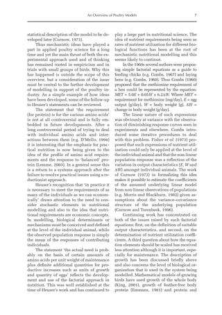
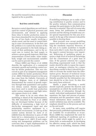
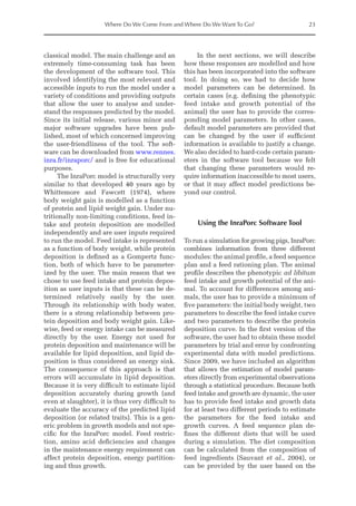

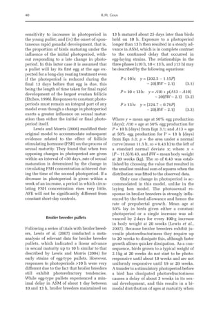
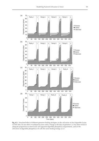
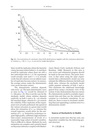
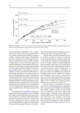
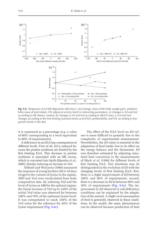
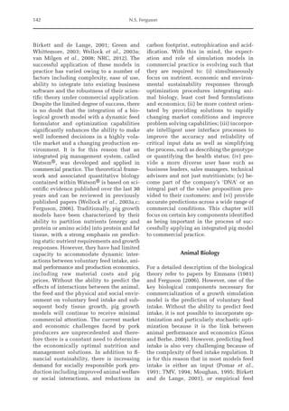
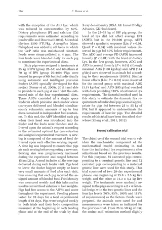
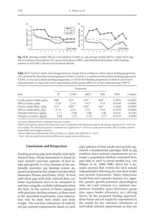
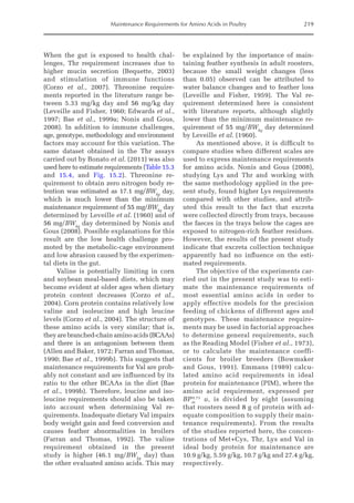
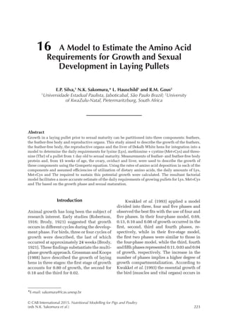
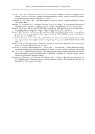
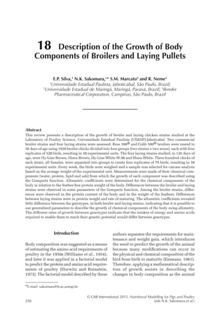
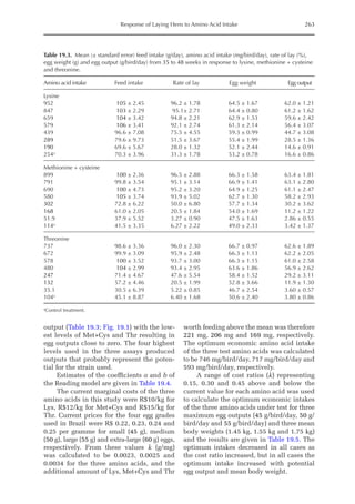
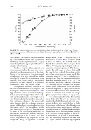
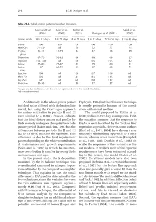
![78 F. Liebert
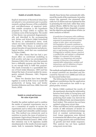
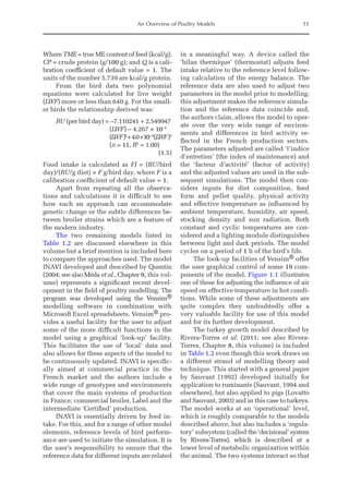
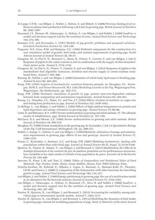
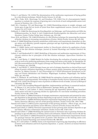
estimation of model parameters (NDmax
T, NMR)
and the evaluation of dietary protein quality
(parameter b), results of these N response ex-
periments are also useful in extending the data-
base of AA requirement studies. For these
applications, a valid definition of the limiting
AA in the diet under study is a prerequisite.
In this case, the shape of the NR-curve is
not only a function of NI, but also of the daily
intake of the limiting AA (LAAI) as a part of
the feed protein fraction. For that important
application, Eqn 6.1 is logarithmically trans-
formed (natural logarithm, ln), providing
Eqns 6.3 and 6.4, respectively:
NI = [lnNRmax
T – ln(NRmax
T – NR)]:b
(6.3)
b = [lnNRmax
T – ln(NRmax
T – NR)]:NI
(6.4)
The model parameters NRmax
T and NMR
for the genotype and the observed data for
NR are used to calculate NI and b, respect-
ively. The derived NI (Eqn 6.3) gives the
daily quantity of dietary protein (in terms
of NI as defined above) needed to yield the
intended level of growth performance (in
terms of NR, as defined above) at a given or
observed dietary protein quality (in terms of
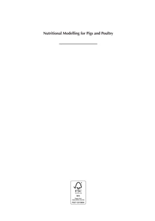
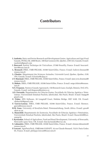
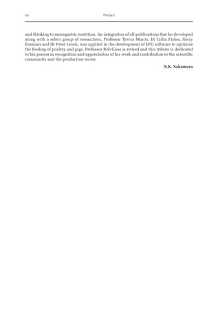
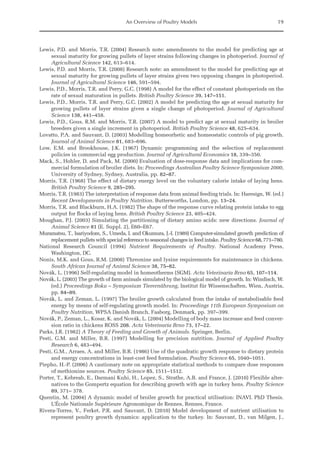
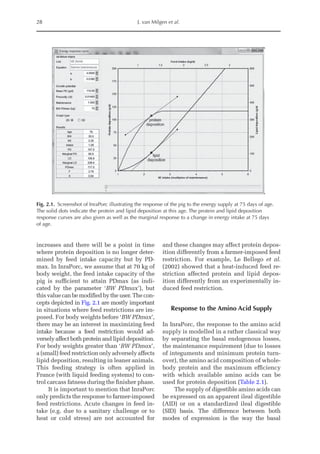
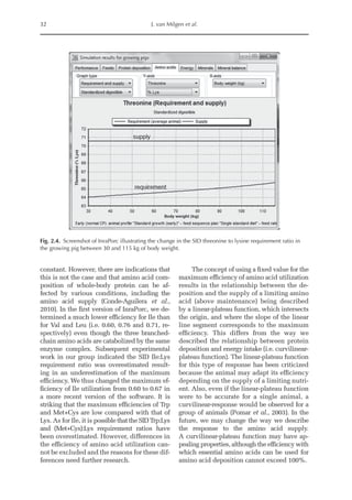
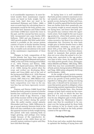
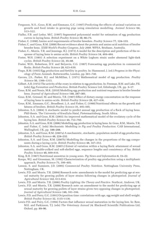
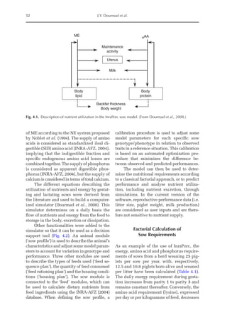
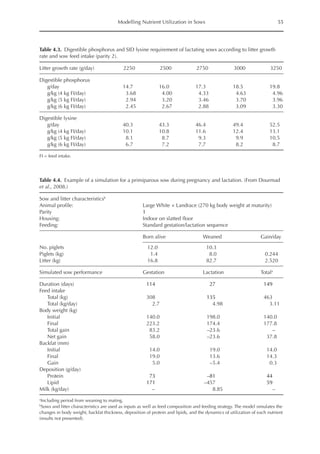
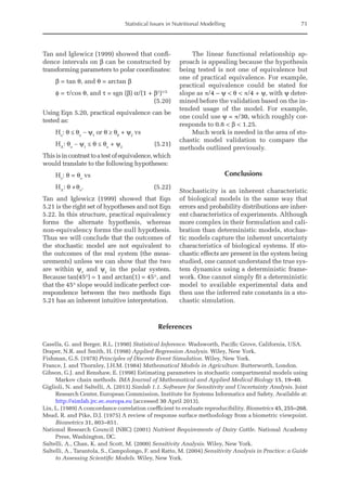
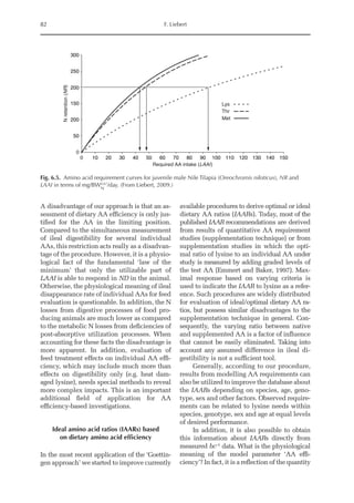
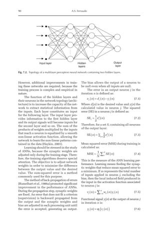
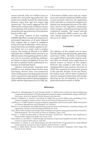
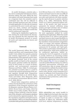
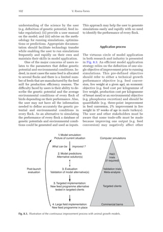
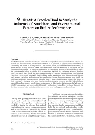
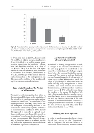
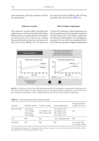
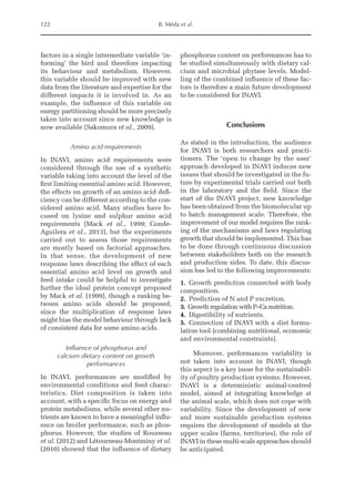
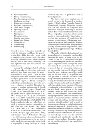
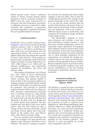
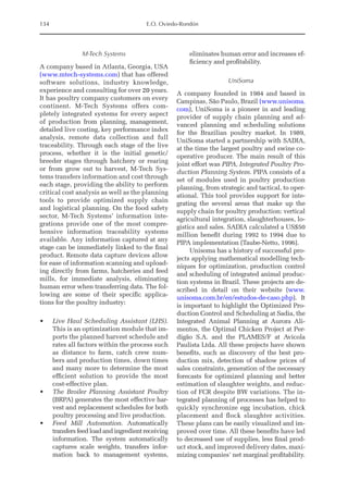
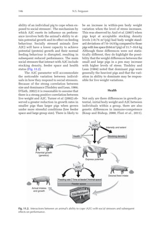
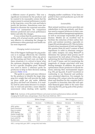
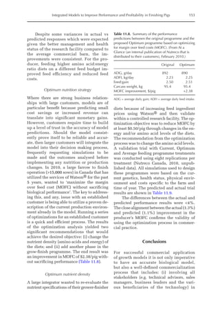
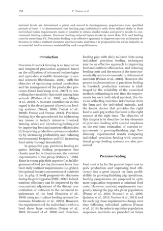
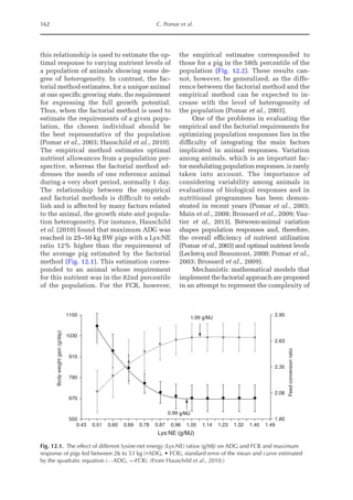
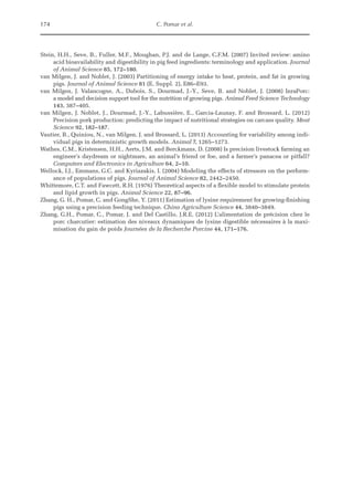
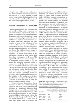
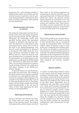
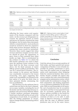
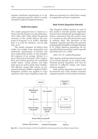
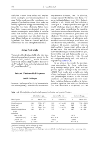
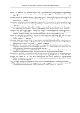
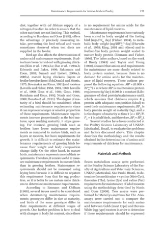
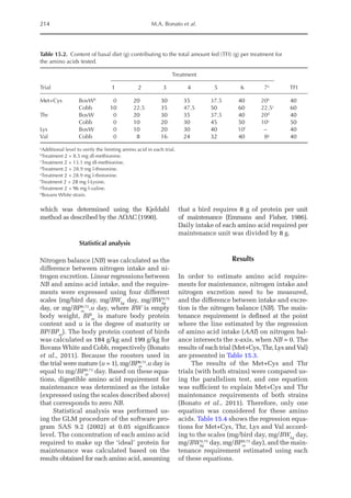
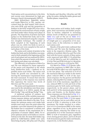
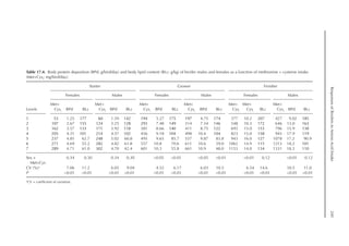
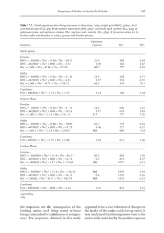
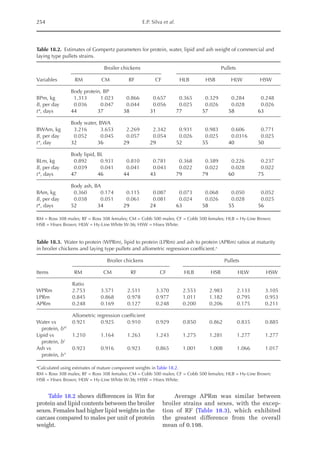
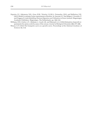
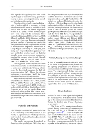
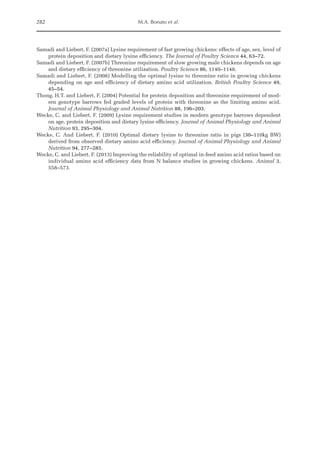
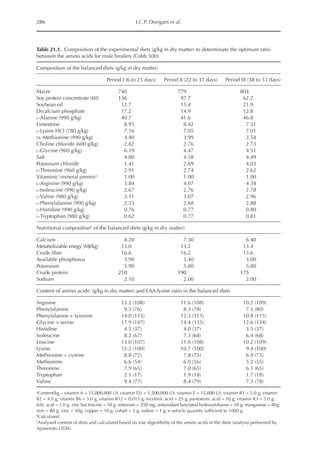
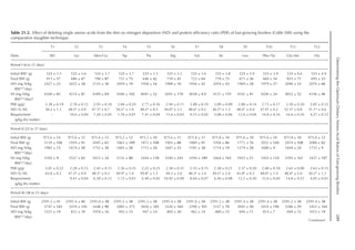
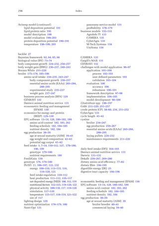
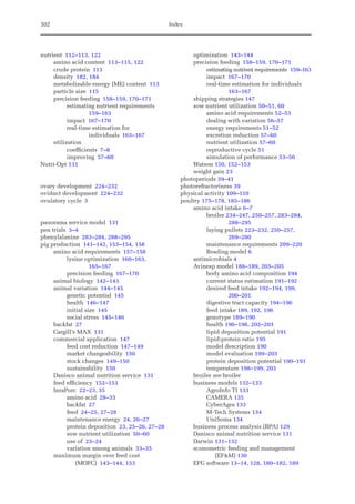
Table 6.3. Diet composition and analysed nutrients of the experimental diets (g/kg as fed basis) with lysine
in limiting position. (From Experiment 1, starter period, Pastor et al., 2013.)
Ingredient N1 N2 N3 N4 N5 N6 N7 N8
Wheat starch 794 691 587 484 308 205 103 0.00
Wheat 72.4 121 169 217 265 314 362 410
SPC 61.8 103 144 185 226 268 309 350
Wheat gluten 10.5 17.4 24.4 31.4 38.4 45.3 52.3 59.3
Fish meal 6.43 10.7 15.0 19.3 23.6 27.9 32.2 36.4
DCP 28.5 26.0 23.5 21.0 18.5 16.0 13.5 11.0
Soybean oil 10.0 13.5 17.0 20.3 97.0 99.5 103 105
Premix 10.0 10.0 10.0 10.0 10.0 10.0 10.0 10.0
NaCl 2.50 2.50 2.50 2.40 2.30 2.20 2.10 2.06
CaCO3
2.30 3.20 4.00 4.70 5.70 6.50 7.20 8.00
dl-Met 0.90 1.51 2.11 2.71 3.32 3.92 4.52 5.12
l-Val 0.30 0.50 0.70 0.89 1.09 1.29 1.49 1.69
l-Thr 0.18 0.29 0.41 0.53 0.65 0.76 0.88 1.00
l-Trp 0.01 0.02 0.02 0.03 0.04 0.05 0.05 0.06
Analysed (g/kg DM)
Crude ash 5.03 5.30 5.55 5.78 6.01 6.26 6.51 6.77
Crude protein 6.46 10.8 15.2 19.7 24.1 28.6 33.2 37.8
Crude fat 1.43 1.99 2.56 3.11 11.6 12.1 12.7 13.3
Crude fibre 0.79 1.04 1.29 1.55 1.76 2.03 2.28 2.55
Starch 74.5 69.2 64.0 58.7 46.5 41.2 35.7 30.2
ME (MJ/kg DM)1 14.18 14.18 14.18 14.18 15.74 15.74 15.74 15.74
a
Calculated, based on WPSA (1984).
Table 6.4. Summarized results of protein quality assessment of lysine limiting chicken diets with graded
dietary protein supply. (From Experiment 1, starter and grower period, Pastor et al., 2013.)
Diet N1 N2 N3 N4 N5 N6 N7 N8
Starter period
b-value (b·10–6
) 196 –a
219 213 200 192 203 204
Grower period
b-value (b·10–6
) 197 197 196 198 195 202 206 187
a
Not detectable, outliers due to feed refusal.](https://image.slidesharecdn.com/nutritionalmodellingforpigsandpoultry-240127070709-ba59d9b4/85/Nutritional-modelling-for-pigs-and-poultry-pdf-93-320.jpg)
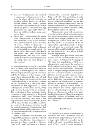
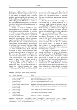
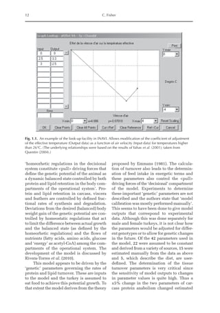
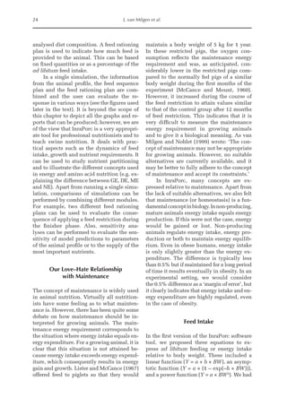
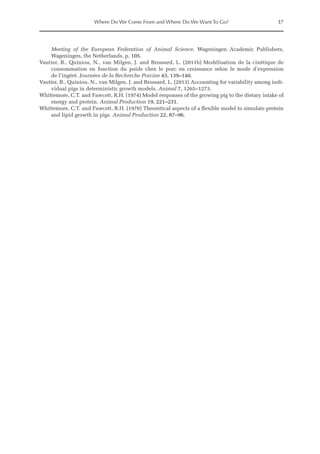
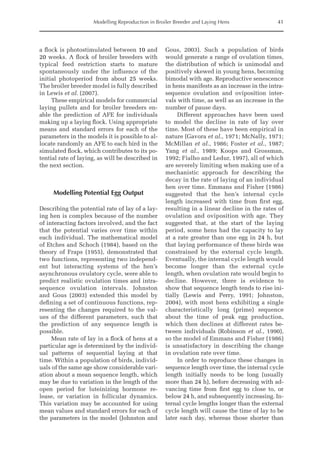
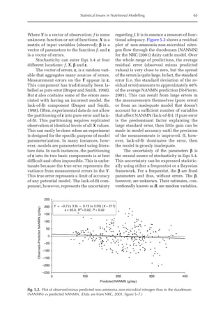
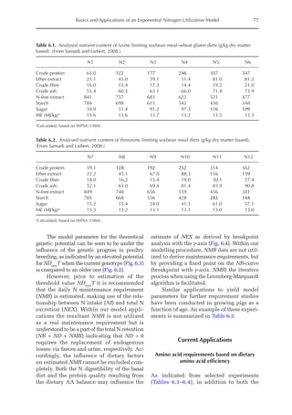
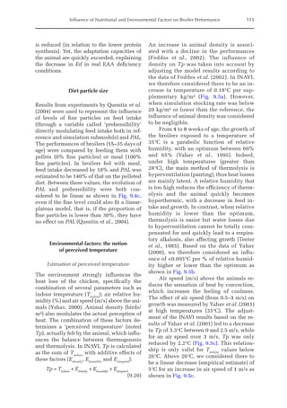
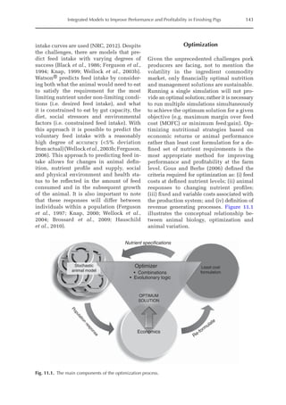
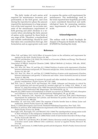
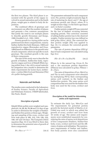
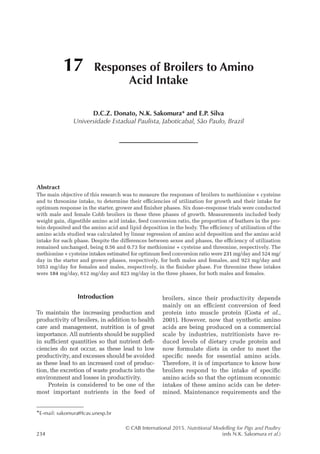
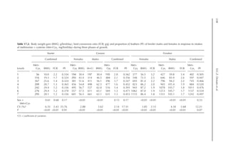
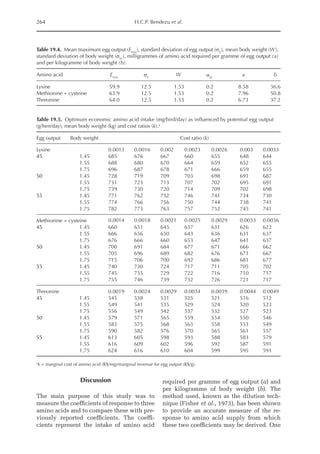
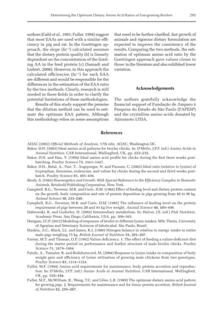
![80 F. Liebert
the animal’s response (ND, NR) generally N
balance or N deposition data from body ana-
lyses are useful. However, factors influen-
cing each of the above procedures may yield
differing results for N balance and N depos-
ition, respectively. This fact is well known
among scientists working in this field, but a
solution to the problem has not as yet been
found. This problem is not specifically re-
lated to the ‘Goettingen approach’ and con-
sequently it will not be discussed further. To
eliminate possible effects of such discrepan-
cies between procedures when quantifying
ND, only applications in growing chickens
and fattening pigs utilizing N balance studies
will be presented below.
Equations 6.1–6.4 have demonstrated
earlier model applications where the main
focus was on questions of complex protein
evaluation and where the AA composition
of the feed protein was not of top priority.
When the emphasis of the model changes
to AA-based applications a further import-
ant transformation is required: the func-
tion needs to be adapted because the inde-
pendent variable determining the resultant
dietary protein quality (b) is the concen-
tration of the limiting AA in the dietary
protein (c). This fundamental connection,
already discussed above, needs to be
‘translated’ into the traditional model ap-
plications.
The ‘key-translator’ to provide this pre-
condition is Eqn 6.5, in which the daily in-
take of the LAA from NI and dietary concen-
tration of the LAA in the feed protein is
calculated:
LAAI = (NI·16):c (6.5)
Where LAAI = daily intake of the LAA in mg/
BWkg
0.67
; c = concentration of the LAA in the
feed protein in g/16g N; and NI = according to
Eqn 6.2.
NR = NRmax
T (1 − e−LAAI·16·b:c
) (6.6)
Where b:c (= bc–1
) = observed dietary
efficiency of the LAA; LAAI = according to
Eqn 6.5; NR = according to Eqn 6.2.
Logarithmic transformation of Eqn 6.6,
according to the mathematical treatment of
Eqn 6.1 as earlier described, yields the basic
Eqn 6.7, which is generally applied for as-
sessing quantitative AA requirements. An
important precondition is that experimental
data are available that describe the NR re-
sponse to a defined intake of limiting AA
(LAAI) at a defined dietary efficiency of the
LAA (bc–1
):
LAAI =
[lnNRmax
T − ln(NRmax
T − NR)]:
16bc−1
(6.7)
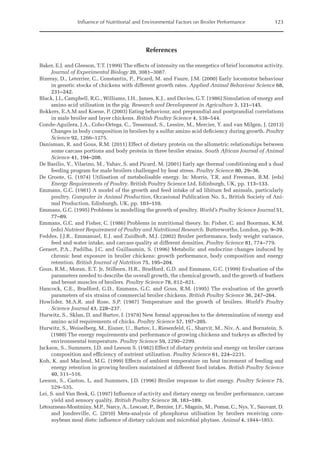
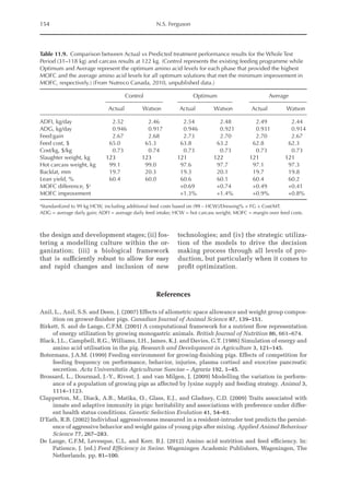
As pointed out with Eqn 6.3 this applica-
tion, which makes use of increasing perform-
ance over a desired range of NR, is of great
interest for tabulating individual AA re-
quirements. Consequently, it is crucial to
plot the desired range as a percentage of
NRmax
T (or NDmax
T) and to utilize the abso-
lute daily deposition data for further model
calculation of AA requirements taking into
account the dietary AA efficiency. An ex-
tended example of this application for grow-
ing fattening pigs is summarized in Table 6.6,
which also shows that the dietary efficiency
of the AA under study can be modulated.
Therefore, an observed value for the dietary
AA efficiency could be increased or lowered
but also gradually changed (Table 6.6) to
express the implications on derived AA
requirements.
Equation 6.7 makes it possible to derive
requirement data for individual AAs under
the precondition that their efficiency (bc–1
)
was measured and validated in a limiting
position of the protein under study. The
question arises as to how this validation
could be achieved. In the case of lysine-,
methionine- or threonine-limiting diets,
based on knowledge of their quantitative and
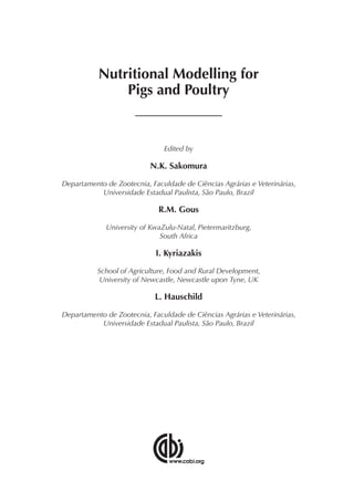
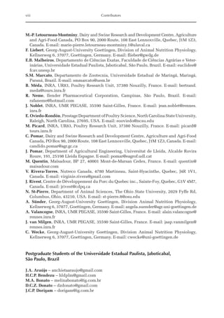
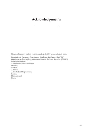
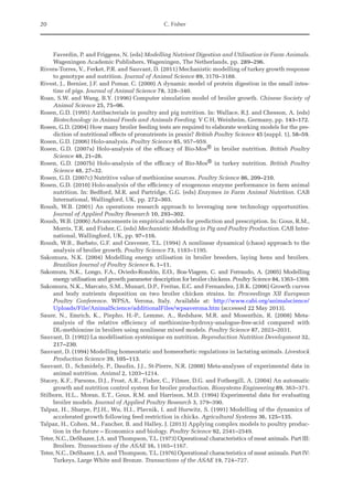
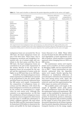
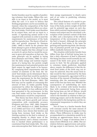
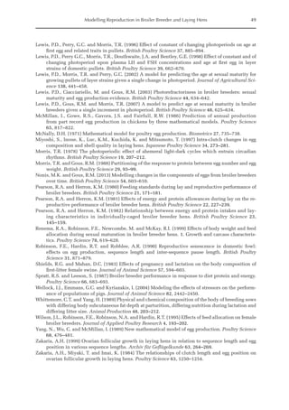
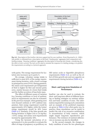
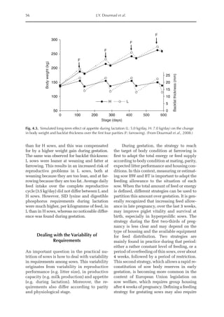
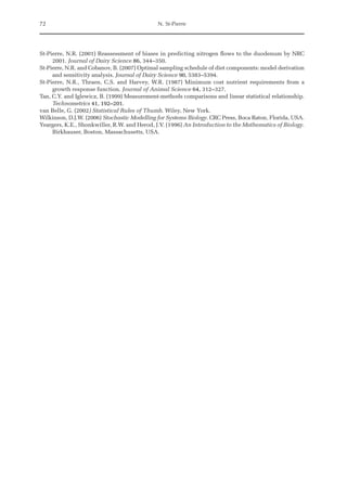
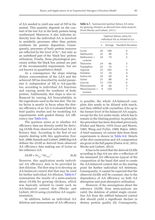
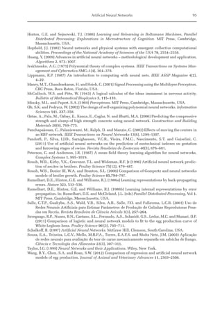
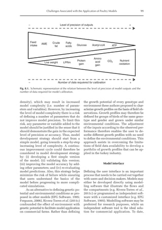
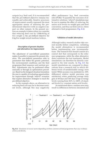
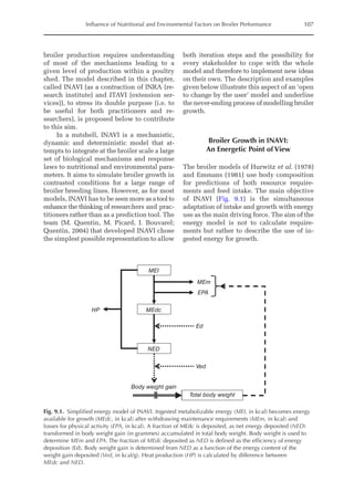
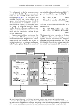
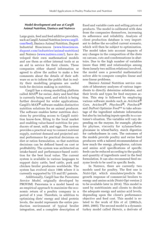
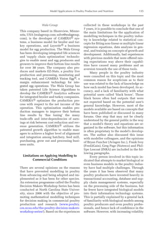
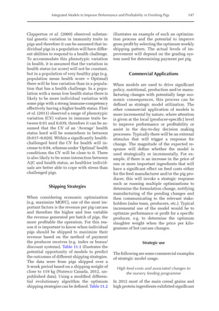
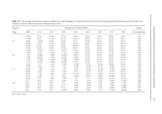
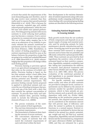
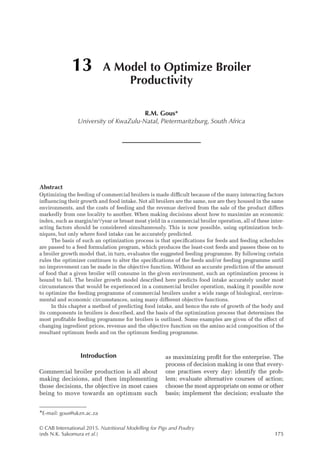
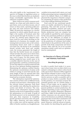
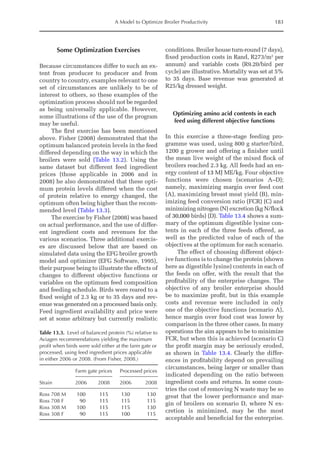
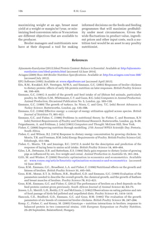
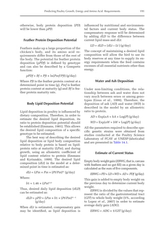
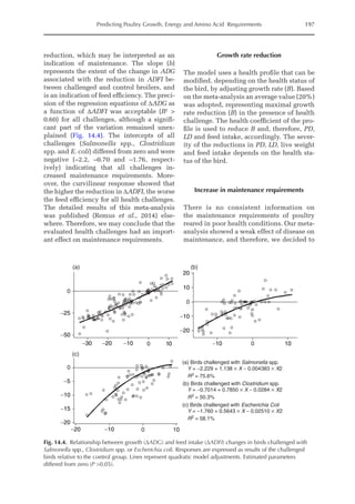
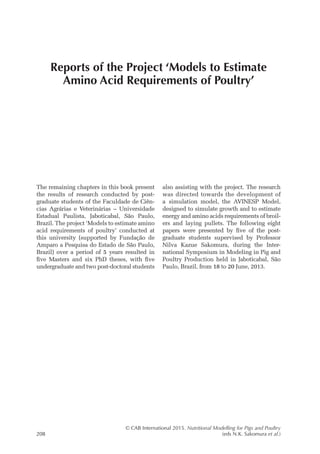
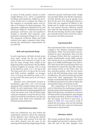
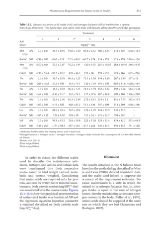
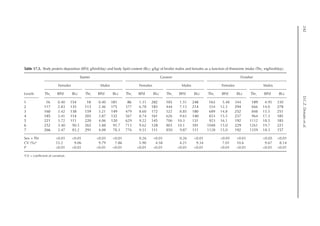
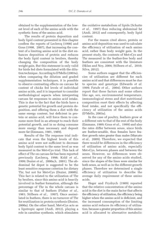
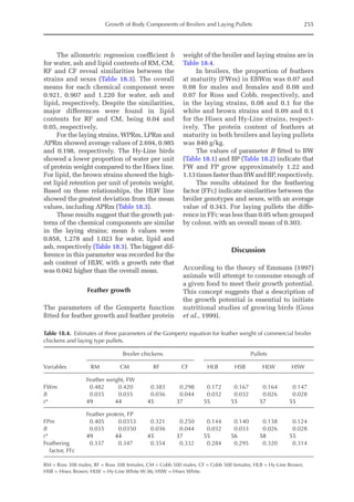
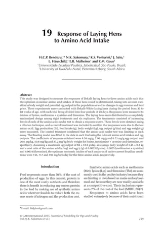
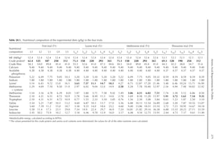
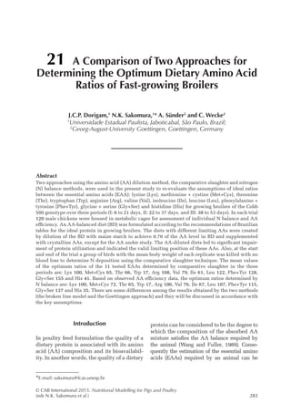
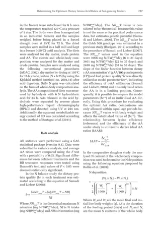
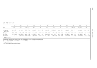
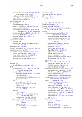
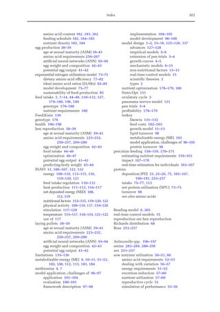
Table 6.5. Observed model parameters (NMR,NRmax
T)
for modern genotype growing barrows depending
on BW. (From Wecke and Liebert, 2009.)
Body
weight (kg)a
NMRb
(mg/BWkg
0.67
)
NRmax
Tb,c
(mg/BWkg
0.67
)
31.9 424 4124
51.6 399 3365
75.5 368 2732
95.4 342 2352
113.8 318 2067
a
Mean BW of the pigs during experimental periods.
b
NMR (mg/BWkg
0.67
) = –1.2863 × BW (kg) + 464.78.
c
NRmax
T (mg/BWkg
0.67
) = –1619.3 × ln BW (kg) + 9733.6.](https://image.slidesharecdn.com/nutritionalmodellingforpigsandpoultry-240127070709-ba59d9b4/85/Nutritional-modelling-for-pigs-and-poultry-pdf-95-320.jpg)
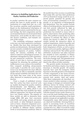
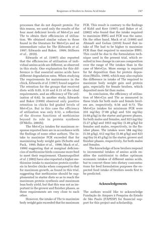
![194 L. Hauschild et al.
composition (ideal protein) to supply its main-
tenance requirements, and Pm is protein
weight at maturity (kg).
In this equation, maintenance require-
ments are related to body protein content,
which is more appropriate to express re-
quirements, because lipid content may be
different even among birds with similar
body weights.
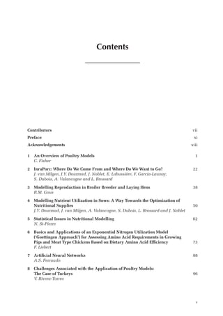
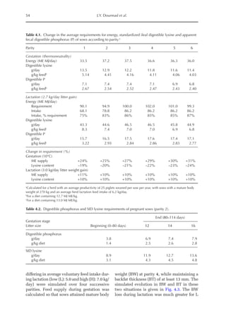
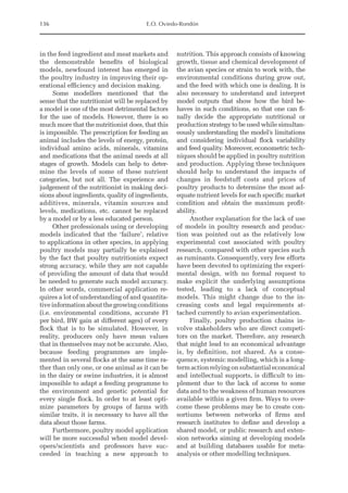
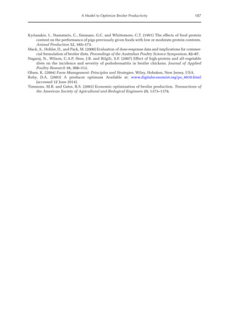
In order to determine maintenance re-
quirements for each amino acid using this
approach, the equation considers body pro-
tein amino acid profile (AAb), as shown in
Table 14.2.
AAm = [(Pm–0.27
) + (0.08 × Pt × AAb)]
(mg/day)
Where AAm is the requirement of a specific
amino acid (AA) for maintenance.
Another important aspect of the model
is that maintenance and body growth com-
ponents were divided into specific ratios to
feather-free body and to feathers, because
feather growth characteristics are different
from the rest of the body and are influenced
by genotype, sex and age, among other factors
(Emmans and Fisher, 1986). Protein require-
ments for feather maintenance are considered
to be proportional to feather losses (Martin
et al., 1994). According to Emmans (1989)
these losses are equivalent to 0.01g/g of
feathers daily. Thus, amino acid require-
ments for feather maintenance (AAmf) were
calculated as:
AAmf = 0.01 × FPt × AAf (mg/day)
Where AAf is amino acid content of feather
protein (Table 14.2).
In order to determine amino acid re-
quirements for growth the factorial equation
takes into account the amino acid profiles
of both body and feather protein and an effi-
ciency of amino acid utilization for body
and feather protein deposition of 0.8. Con-
sidering all the above-mentioned aspects, a
general equation was built to estimate amino
acid requirements:
AA = AAm + AAmf + (AAb × PD/k)
+ (AAf × PDf/k) (mg/day)
Where AA is digestible amino acid require-
ment and k is the efficiency of the utiliza-
tion of that amino acid for feather-free body
deposition and feather deposition. The model
estimates the requirements for the following
amino acids: lysine, methionine, methio-
nine + cystine, threonine, tryptophan, isoleu-
cine, leucine, valine, phenylalanine, histidine
and arginine.
In order to determine the amount of
feed required for potential growth the di-
gestible amino acid content (AAd) must be
known. Therefore, the desired intake to
supply amino acid requirements is calcu-
lated as:
dFIAA
= AAd/AA (g/day)
Physical Capacity of the
Digestive Tract
Nutrient intake by poultry may be limited
by dietary fibre content due to the physical
limitations of their digestive tract, particu-
larly during early growth stages. To account
for the effect of dietary fibre on feed intake,
a meta-analysis was performed by taking
into account four studies (Nascimento et al.,
1998; Bellaver et al., 2004; Montazer-Sadegh
et al., 2008; Sara et al., 2009). In those stud-
ies, broilers were fed diets with different
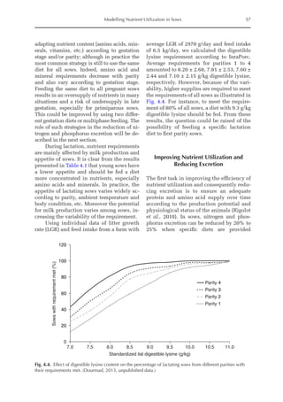
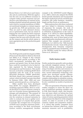
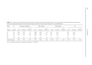
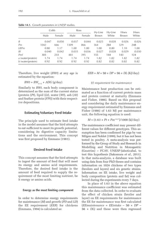
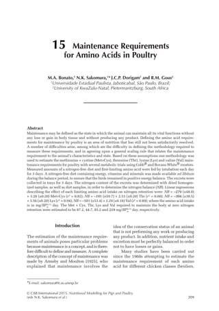
Table 14.2. Amino acid composition of the body
and feather for chickens.a
(From Stilborn et al.,
1997, 2010.)
Amino acid Body Feather
Arginine 6.51 6.65
Cystine 1.00 7.46
Histidine 2.41 0.71
Isoleucine 3.94 4.60
Leucine 7.19 7.87
Lysine 6.87 1.97
Methionine 2.16 0.69
Phenylalanine 3.79 4.66
Tyrosine 2.74 2.59
Threonine 4.07 4.80
Tryptophan 0.69 0.74
Valine 4.67 6.14
Alanine 6.26 4.09
Glycine 7.86 7.04
a
Means for male and female.](https://image.slidesharecdn.com/nutritionalmodellingforpigsandpoultry-240127070709-ba59d9b4/85/Nutritional-modelling-for-pigs-and-poultry-pdf-209-320.jpg)
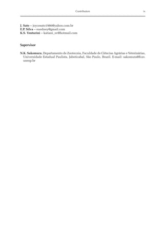
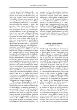
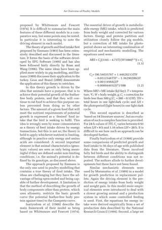
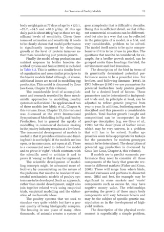
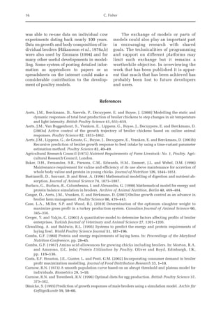
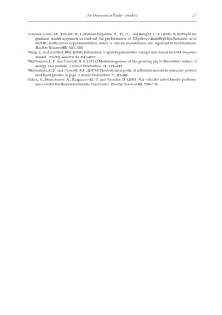
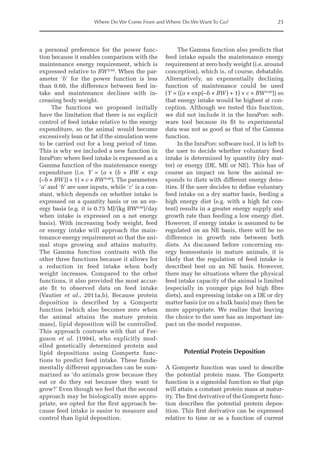
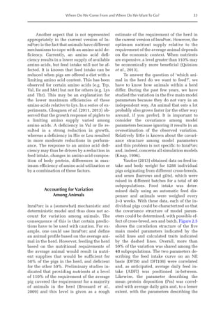
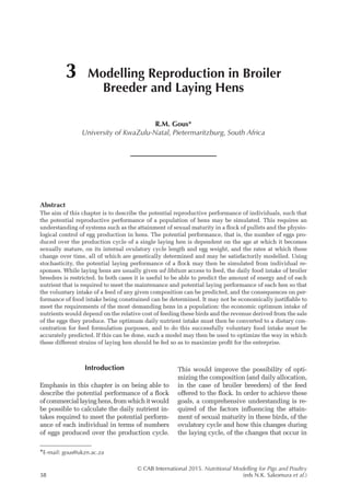
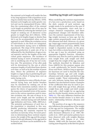
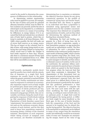
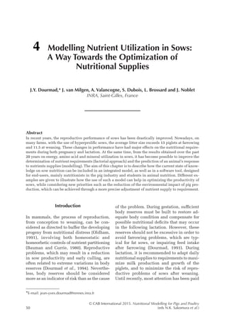
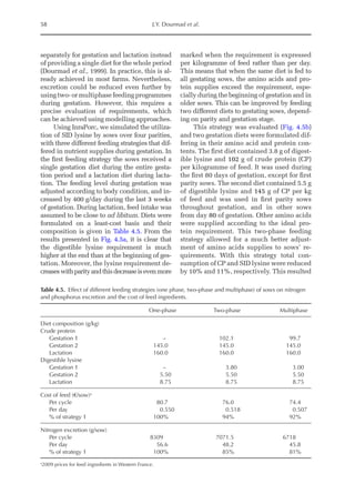
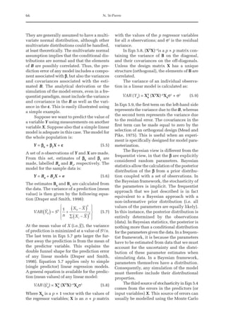
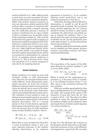
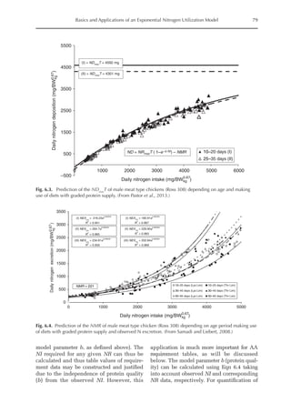
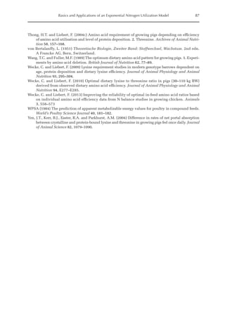
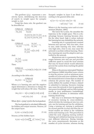
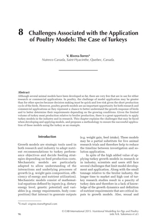
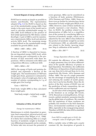
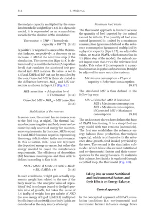
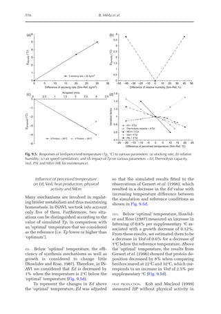
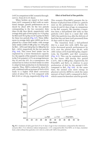
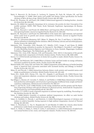
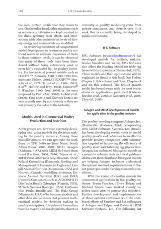
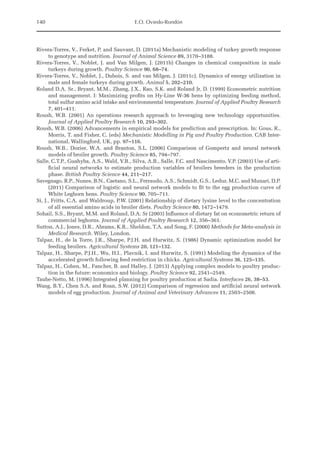
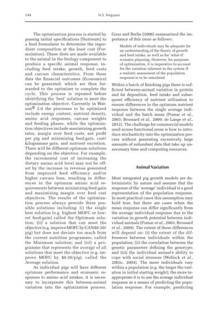
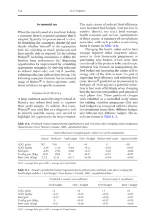
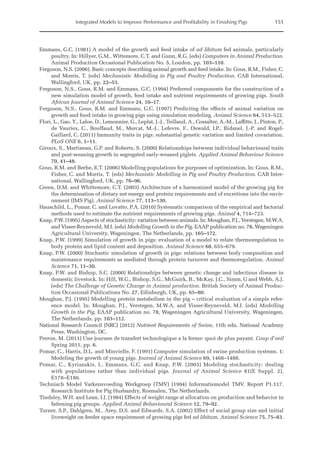
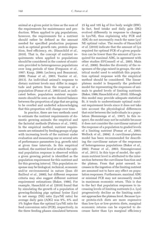
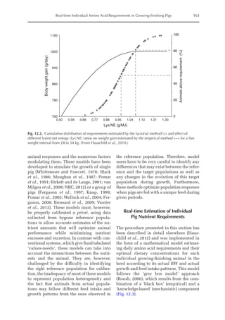
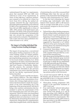
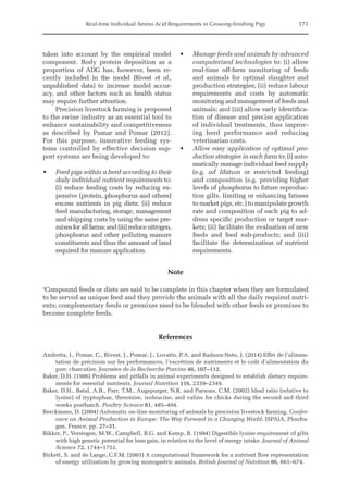
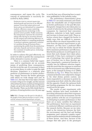
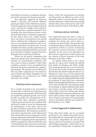
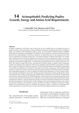
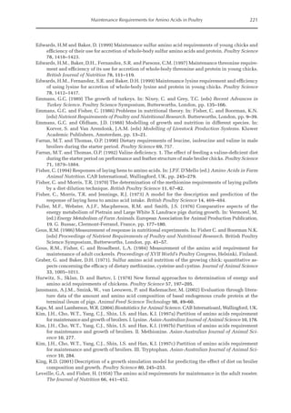
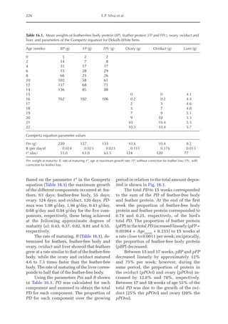
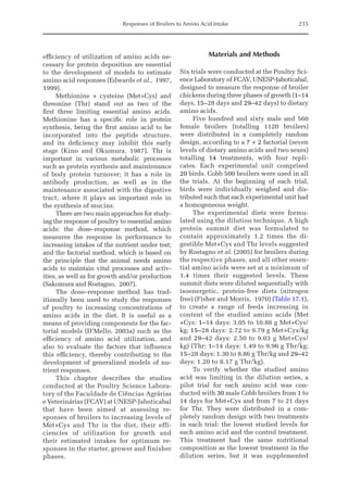
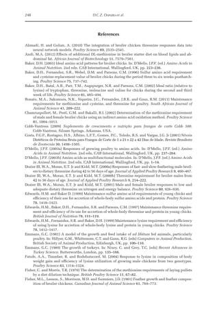
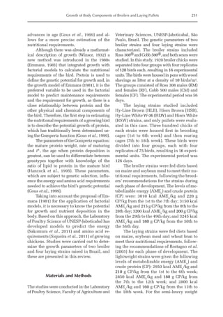
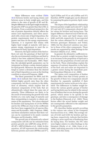
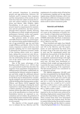
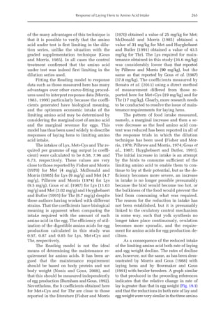
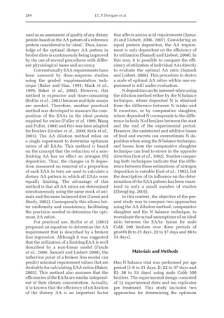
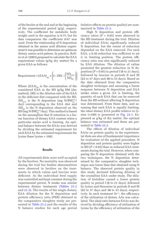
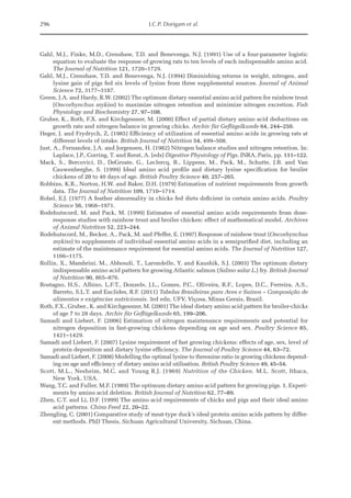
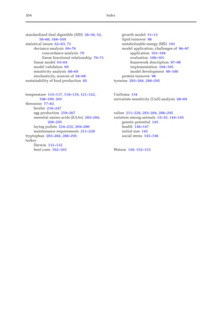
![Predicting Poultry Growth, Energy and Amino Acid Requirements 195
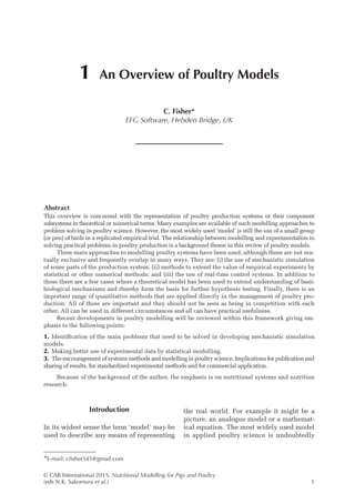
total dietary fibre contents (TDF). Feed in-
take reduction (rFI) of birds fed diets with
TDF increasing levels was expressed as a
percentage relative to a control diet (con-
ventional diet containing corn and soybean
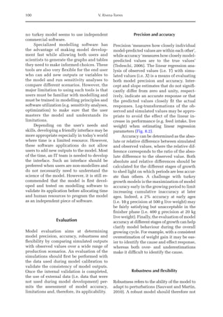
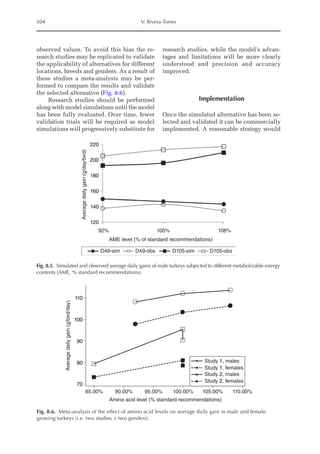
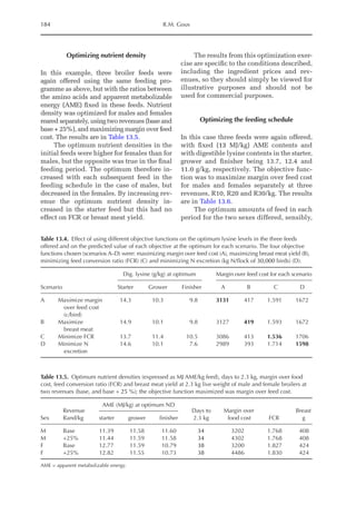
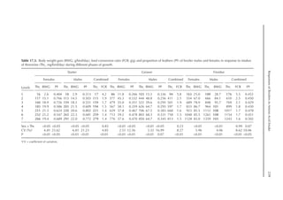
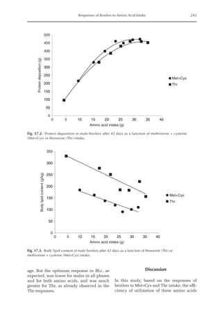
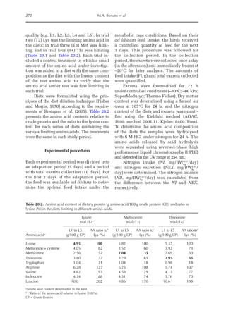
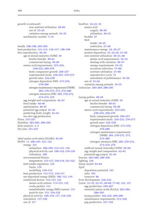
meal). Data on rFI were regressed against
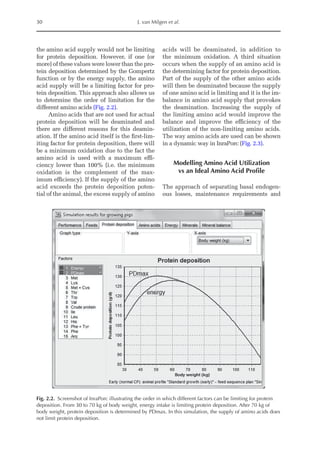
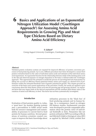
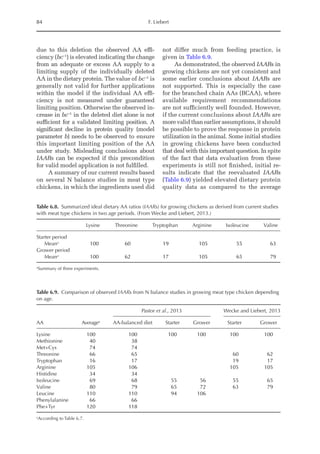
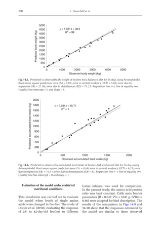
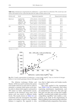
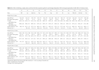
TDF content (Fig. 14.3).
The equation estimates feed intake reduc-
tion as a function of TDF percentage in the diet:
rFI =
[100 + (17.6 + 0.52 × (36 –TDF))]/
100 (%)
Total dietary fibre content (TDF) of the feed-
stuffs in the model may be obtained using
the equation of Bellaver et al. (2004):
TDF = 2212.56 – 0.0492 × EM – 1.103 ×
ADF – 7.053 × EE – 9.196 × MM(%)
Where ADF is acid-detergent fibre, EE is
ether extract and MM is ashes.
In order to correct feed intake according
to physical capacity, based on the effect of
dietary fibre, the following equation is applied:
cFI = rFI × mFI (g/day)
Where cFI is feed intake corrected for phys-
ical capacity and mFI is maximum feed in-
take. In order to calculate mFI, daily feed
intake was related to protein weight (x).
The equation for each genetic strain is pre-
sented below:
Cobb male: mFI = –0.0006279x2
+ 0.71542x + 1.7489 (g/day)
Cobb female: mFI = –0.001146346x2
+ 0.8735x + 7.7553 (g/day)
Ross male: mFI = –0.000482069x2
+ 0.66129x + 8.708551 (g/day)
Ross female: mFI = –0.0007711x2
+ 0.74407x + 9.24998 (g/day)
Hy-Line white: mFI = –0.0002677x2
+ 0.34919x + 6.2229 (g/day)
Hy-Line brown: mFI = –0.000666269x2
+ 0.44387x + 5.6498 (g/day)
Hisex white: mFI = –0.0005078x2
+ 0.40907x + 5.07180 (g/day)
Hisex brown: mFI = –0.0003668x2
+ 0.38615x + 4.89426 (g/day)
One aspect that must be considered in the
model is the hypothesis confirmed by Gous
et al. (2012) that chickens of any age attempt
to maintain the body lipid to protein ratio
determined by their genetic potential by
long-term regulation mechanisms. Therefore,
feed intake will always depend on the bird’s
current state. According to this theory, which
was first proposed by Emmans (1981), when
an animal has more body lipid than its genet-
ically determined lipid:protein ratio, the
extra amount of lipid will be used as an en-
ergy source whenever possible. In a recent
study, Gous et al. (2012) observed that for a
given feed, body lipid reserves in broilers in-
creased at first due to the need to consume
Fig. 14.3. Effect of total dietary fibre on broiler feed intake.
5
0
0
Feed
intake
reduction
(%)
Total dietetic fibre (%)
−5
−10
−15
−20
–25
10 20 30 40 50](https://image.slidesharecdn.com/nutritionalmodellingforpigsandpoultry-240127070709-ba59d9b4/85/Nutritional-modelling-for-pigs-and-poultry-pdf-210-320.jpg)

Maximum EHL is usually constant and sev-
eral times greater than EHLmin
. In the study
of Simmons et al. (1997) an equation was
derived to calculate the external effects of
temperature and ventilation on body heat
production. That study was carried out to
determine latent HP in 35- and 42-day-old
broilers subjected to different air velocities
and temperatures under conditions similar
to those found in commercial settings. The
authors estimated 12 polynomial equations
to predict latent HP as a function of air
speed and temperature. Those equations
were re-parameterized in a single equation
to predict latent HP (kJ/day) as a function of
air velocity, temperature (T, ºC) and body
weight.
EHLmax
=
BW × [9.4434 × (Vel – 0.0215)
× T] (kJ/day)
Where Vel = air velocity (m/s).
In order to determine thermal environ-
ment effects on growth rate and feed intake,
THP is compared with THLmax
and THLmin
.
THP is calculated as the difference between
energy intake and energy retention for pro-
tein and fat deposition:
THP = (aFI × ME) – [(23.8 × PD)
+ (39.6 × LD)] (kJ/day)
Comparing maximum or minimum THL with
THP indicates whether the birds are too
hot, too cold or comfortable, and enables](https://image.slidesharecdn.com/nutritionalmodellingforpigsandpoultry-240127070709-ba59d9b4/85/Nutritional-modelling-for-pigs-and-poultry-pdf-213-320.jpg)
![Predicting Poultry Growth, Energy and Amino Acid Requirements 199
adequate voluntary feed intake and growth
rates to be calculated.
Response to environmental conditions
When heat produced by the bird is greater
than the maximum it can lose (THP THLmax
)
to the environment the bird is hot and, there-
fore, will attempt to reduce THP to THLmax
.
In this case, feed intake declines to main-
tain the heat production balance:
aFI = dFIe
– (THP – THLmax
)/ME (g/day)
The impact of aFI reduction on PD and LD
depends on whether amino acid intake is
still sufficient to meet pPD (PDAA
) require-
ments, given that PD is determined by:
PDAA
= [(AAintake – AAm) × k]/AAb
(g/day)
Lipid deposition (LD) is estimated as the
difference between energy intake and energy
retained for PD and lost as heat.
LD = [(aFI × ME) – THP – (23.8 × PD)]/
39.6 (g/day)
When the amount of heat loss is greater than
heat production (THP THLmin
) the bird is
cold. In this case extra heat will be neces-
sary to maintain body temperature and en-
sure THP = THLmin
. The energy difference
between THLmin
and THP causes mainten-
ance requirements to increase and feed in-
take will therefore increase by:
ExtraFI = (THLmin
– THP)/ME (g/day)
If (ExtraFI + aFI) cFI (bulk constraint)
then feed intake will decline to cFI, and PD
and LD will be adjusted accordingly, as pre-
viously discussed under constrained feed
intake.
Model Evaluation
Under adequate nutritional supply
Estimating growth and body composition
The ability of the model to estimate body
weight and cumulative feed intake (CFI)
was evaluated by comparing measured
and predicted data. The model was cali-
brated to predict the observed BW and CFI
of each genetic strain. All strains were fed
according to the feeding phases applied in
the original experiment. All feeds con-
tained 11.5 MJ EE/kg and were assumed to
contain all other nutrients in excess, in-
cluding Lys. For the evaluation, observed
and predicted data for each strain were
compiled according to chicken strain
(broiler and pullet). The quality of fit was
tested by the procedure of Theil (1966)
in which the mean squared prediction
error (MSPE) is calculated as the sum of
squares of differences between simulated
and observed measurements divided by
the number of experimental observations.
MSPE was decomposed into error in cen-
tral tendency, error due to regression (ER)
and error due to disturbances, and expressed
as MSPE%, as suggested by Benchaar et al.
(1998).
Simulated and observed values were
similar across all feeding periods both for
body weight and cumulative feed intake of
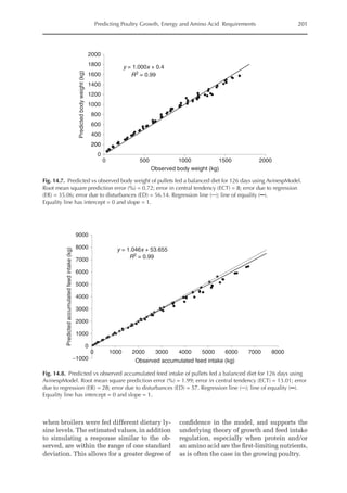
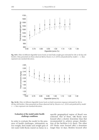
broilers and pullets (Figs 14.5, 14.6, 14.7
and 14.8). Model accuracy, as estimated by
MSPE, was 0.01 (broilers) and 0.72 kg (pul-
lets) for BW and 0.68 (broilers) and 1.99 kg
(pullets) for CFI. Deviations between ob-
served and predicted performance values
were small, which is consistent with the
fact that model parameters were estimated
for each strain and chicken type. However,
the slope between the predicted and ob-
served BW (broilers) and CFI (pullets) was
1.04, which is higher than 1 (P 0.001), in-
dicating that the model slightly underesti-
mated these parameters during the first
feeding phase, and slightly overestimated
them in older birds. In fact, more than 20%
of the observed error between predicted and
observed BW and CFI is given by the diffe-
rence between the slopes (ER error).
Because unique parameters (mainten-
ance coefficient, energy cost for protein and
lipid deposition, etc.) were applied both for
meat-type and layer-type chickens, except
for those used for bird description, the
model was able to obtain growth and intake
estimates very close to observed values.](https://image.slidesharecdn.com/nutritionalmodellingforpigsandpoultry-240127070709-ba59d9b4/85/Nutritional-modelling-for-pigs-and-poultry-pdf-214-320.jpg)

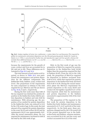
![Model to Estimate the Amino Acid Requirements in Laying Pullets 225
in the model. The model is described by
Eqn 16.3:
AAI =
[(AAmc
× BPm0.73
× u)
+ (FPL × FP × AAf
)] + [(AAc
× PDc
)/k + (AAf
× PDf
)/k + AAc
× (PDOva
+ PDOvi
+ PDLiv
)/k](16.3)
Where AAI is the digestible amino acid
requirement (mg/day); AAmc
is the amino
acid requirement for the maintenance of
feather-free body protein (mg × BPm0.73
× u);
BPm0.73
is the metabolic body protein weight
at maturity (kg); u is the degree of maturity
of feather-free body protein (u = BPt/BPm);
FPL is the feather protein loss (0.04 g/day);
FP or FPc is the feather protein weight (g/day);
AAf is the amino acid content of feather pro-
tein (mg/g); AAc
is the amino acid content of
feather-free body protein (mg/g); PDc
is the
rate of deposition of feather-free body (g/day);
PDf
is the rate of protein deposition in the
feathers (g/day); PDOva
is the rate of protein
deposition in the ovary (g/day); PDOvi
is
the rate of protein deposition in the oviduct
(g/day); PDLiv
is the rate of protein deposition
in the liver (g/day); and k is the efficiency
of utilization of amino acid for protein de-
position.
Laying hens lose a significant amount
of feathers during growth (Silva, 2012). The
daily loss of feathers may be regarded as the
maintenance requirement for feathers, as sug-
gested by Emmans (1989). The amino acid
composition for feather protein maintenance
was considered to be equal to its concentra-
tion in feather protein.
Coefficients for calculating the mainten-
ance requirements of the feather-free body
for Lys, Met+Cys and Thr were obtained from
studies conducted at UNESP-Jaboticabal. The
Lys requirement was calculated as 174 mg
× BPm0.73
× u (Siqueira et al., 2011), the co-
efficient for Met+Cys requirement was 93.5
and for Thr, 44.7 (Bonato et al., 2011).
The coefficient used to describe the ef-
ficiency of utilization of Lys (kLys
), Met+Cys
(kMet+Cys
) and Thr (kThr
) was 0.80 for all three
amino acids.
The contents of Lys, Met+Cys and Thr
in feathers and in the feather-free body were
measured by Silva (2012) to be 18.7 mg/g,
89.2 mg/g and 44.3 mg/g protein, respectively,
in feathers (AAf
) and 67.8 mg/g, 33.3 mg/g and
40.4 mg/g, respectively, in the feather-free
body (AAc
).
Estimating the requirements
The Lys, Met+Cys and Thr requirements were
estimated by applying the parameters for
Dekalb White hens using the Martin et al.
(1994) model (Model 1) and then making
corrections for feather growth and the inclu-
sion of organs (Model 2).
Model 1: based on Martin et al. (1994)
(M1):
AAI =
[(AAmc
× BPm0.73
× u)
+ (FPL × FP × AAf
)]
+ [(AAc
× PDc
)/k + (AAf
× PDf
)/k](16.4)
Model 2: corrected for feather loss and the
growth of reproductive organs and liver (M2):
AAI =
[(AAmc
× BPm0.73
× u)
+ (FPL × FP × AAf
)]
+ [(AAc
× PDc
)/k
+ (AAf
× PDf
)/k + AAc
× (PDOva
+ PDOvi
+ PDLiv
)/k](16.5)
Results
Description of the growth parameters
The growth parameters for the protein weights
of feathers, feather-free body and ovary, ovi-
duct and liver of Dekalb White hens are given
in Table 16.1. At maturity (Pm) the total pro-
tein weight of the bird was 382 g. Of this, 0.57
corresponded to the feather-free body, 0.35
to feathers, 0.03 to the ovary, 0.03 to the oviduct
and 0.02 to the liver.
The correction for feather loss applied
to the observed weights resulted in a 4% in-
crease in the protein weight of feathers (PFm;
Table 16.1). This correction enabled an ap-
proximation to be made of the real feather
weight, which is of considerable importance
when determining the amount of each amino
acid required for the growth of feathers, espe-
cially cystine.](https://image.slidesharecdn.com/nutritionalmodellingforpigsandpoultry-240127070709-ba59d9b4/85/Nutritional-modelling-for-pigs-and-poultry-pdf-240-320.jpg)
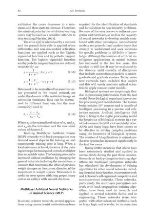
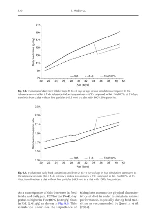
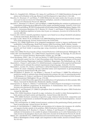
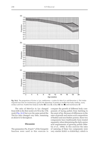
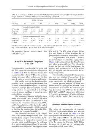
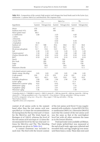
![Model to Estimate the Amino Acid Requirements in Laying Pullets 227
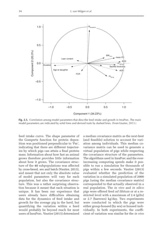
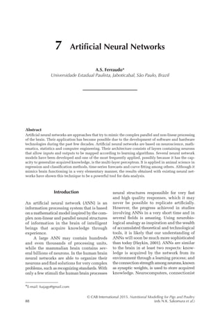
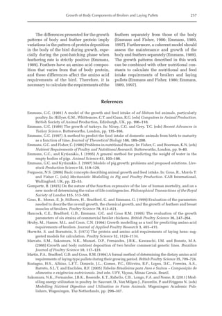
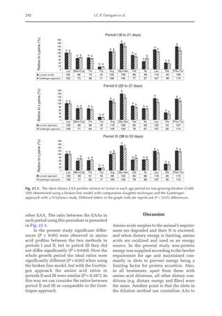
The increase in the proportion of liver
protein (pPLiv) during the growth peak in
the sexual maturity phase is less representa-
tive when the factors are analysed together,
but an analysis of the isolated organ is
shown in Fig. 16.2. A separate approach re-
veals that after the maximum growth rate of
the ovary and oviduct, there was an increase
in pPLiv from the 18th week, according to
the broken line equation: pPLiv%=1.46 –
0.45 × (18 – Age(weeks)
) for Age 18th week,
when Age ≥15th and ≤18th, pPLiv = 1.46.
Models used to estimate amino acid
requirements
Considering the growth parameters and coef-
ficients obtained, the models for Lys, Met+Cys
and Thr are presented below:
For Lys:
AAI =
[(173 × BPm0.73
× u)
+ (0.04 × FP × 18.7)]
+ [(67.8 × PDc
)/0.8
+ (18.7 × PDf
)/0.8 + 67.8
× (PDOva
+ PDOvi
+ PDLiv
)/0.8](16.6)
0.0
0.2
0.4
0.6
0.8
1.0
1 4 7 10 13 16 19 22 25
Relative
deposition
rate
(g/kg)
Age (weeks)
Fig. 16.1. Rate of protein deposition in each of the protein components of the body over time relative to the
total amount deposited. Feather-free body .. . ; feathers . . ; ovary ; oviduct ..............; and
liver .
0.000
0.005
0.010
0.015
0.020
0.025
0.030
0.035
0.040
0.045
0.050
15 17 19 21 23 25
Relative
deposition
(g/kg)
Age (weeks)
Fig. 16.2. Protein deposition in the liver as a proportion (g/kg) of the total amount deposited in the body
(feather-free body + feathers + ovary + oviduct + liver). Observed values ; predicted values .](https://image.slidesharecdn.com/nutritionalmodellingforpigsandpoultry-240127070709-ba59d9b4/85/Nutritional-modelling-for-pigs-and-poultry-pdf-242-320.jpg)
![228 E.P. Silva et al.
For Met+Cys:
AAI =
[(93.5 × BPm 0.73
× u)
+ ( 0.04 × FP × 89.2)]
+ [(33.3 × PDc
)/0.8
+ (89.2 × PDf
)/0.8
+ 33.3 × (PDOva
+ PDOvi
+ PDLiv
)/0.8] (16.7)
For Thr:
AAI =
[(44.7 × BPm0.73
× u)
+ (0.04 × FP × 44.3)]
+ [(40.4 × PDc
)/0.8
+ (44.3 × PDf
)/0.8 + 40.4
× (PDOva
+ PDOvi
+ PDLiv
)/0.8]
(16.8)
Where AAI is the digestible amino acid
requirement (mg/day); 173, 93.5 and 44.7 are
the respective Lys, Met+Cys and Thr require-
ments for maintaining the feather-free pro-
tein body weight; BPm is the protein weight
of the feather-free body at maturity (kg), u is
the degree of maturity of the feather-free body
protein (u = BPt/BPm); 0.04 is the protein
loss of the feathers (0.04 g/day); FP or FPc is
feather protein weight (g/day); 18.7
, 89.2 and
44.3 mg/g are the respective Lys, Met+Cys
and Thr contents in the feather protein; 67.8
mg/g, 33.3 mg/g and 40.4 mg/g are the respect-
ive Lys, Met+Cys and Thr contents in the
protein of the feather-free body; PDc
, PDf
,
PDOva
, PDOvi
and PDLiv
are the respective pro-
tein depositions of the feather-free body,
feathers, ovary, oviduct and liver (g/day); and
0.8 is the efficiency of amino acid utilization
for protein deposition.
Models for determining requirements
The factorial model described estimates the
intake of Lys, Met+Cys and Thr required to
maintain the feather-free body protein, to
meet the requirements for feather loss and
to deposit protein in the feather-free body,
the feathers and the ovary, oviduct and liver
using the value 0.8 for the efficiency of util-
ization of the three amino acids for protein
growth. The weekly requirements through-
out growth are shown in Table 16.2.
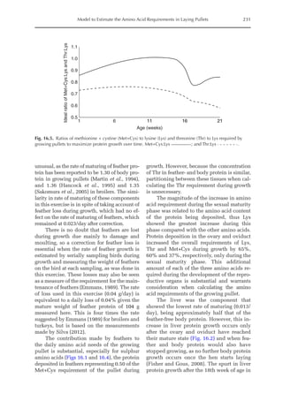
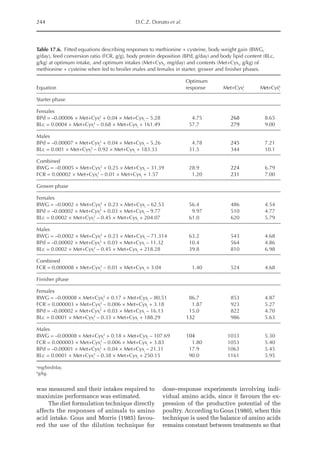
Differences in the estimates of the daily
intakes required for Lys, Met+Cys and Thr
predicted by models M1 and M2 are illus-
trated in Fig. 16.3. The correction for feather
loss is evident to the 13th week of age and
differs for each amino acid. Although the
weekly differences appear to be minimal, the
cumulative differences for Lys, Met+Cys and
Thr to the 13th week of age sum to 6%, 28%
and 18%, respectively.
From the 15th week, the differences
between models M1 and M2 are greater
Table 16.2. Predicted lysine (Lys), methionine + cystine (Met+Cys) and threonine (Thr) requirements
(mg/day) of laying-type pullets during the growing period.
Age Lysine Methionine + cystine Threonine
(Week) M1a
M2b
M1a
M2b
M1a
M2b
1 84 84 71 72 61 61
3 143 144 128 130 106 107
5 193 193 179 182 144 146
7 219 220 209 214 165 167
9 221 222 216 222 166 169
11 207 209 205 211 154 156
13 185 186 182 188 134 136
15 161 165 156 163 112 116
17 139 229 131 179 91 147
19 120 163 108 133 74 101
21 104 116 90 98 59 67
23 93 97 75 79 48 51
25 84 86 63 66 40 42
a
Model 1 based on Martin et al. (1994).
b
Model 2 corrected for feather loss and growth of reproductive organs and liver.](https://image.slidesharecdn.com/nutritionalmodellingforpigsandpoultry-240127070709-ba59d9b4/85/Nutritional-modelling-for-pigs-and-poultry-pdf-243-320.jpg)
![252 E.P. Silva et al.
strains, the following values were used:
2950 kcal AMEn
/kg and 210 g CP/kg from
the 1st to the 6th week; 2850 kcal AMEn
/kg
and 170 g CP/kg from the 7th to the 12th
week; and 2750 kcal AMEn
/kg and 160 g CP/
kg from the 13th to the 18th week.
Every week, the birds were weighed and
sample animals were selected for slaughter
based on the average weight of each experi-
mental unit. After a fasting period of 24 h the
sampled birds were individually weighed
and euthanized using CO2
, and feather sam-
ples were collected. The weight of feathers
was determined by the difference between
the weight of the fasted bird and the weight
of the defeathered carcass.
The defeathered carcasses were ground
to obtain homogeneous samples. An aliquot
of each sample was set aside for subsequent
pre-drying. The samples were then ground in
a micro-mill and analysed for nitrogen con-
tent (Kjeldahl method, crude protein = nitro-
gen × 6.25), ether extract (petroleum ether in
Soxhlet equipment), dry matter (oven at
105°C) and ash (muffle at 550°C). The feather
samples were chopped with scissors and sub-
jected to the same chemical analyses.
To describe the growth of the major body
components, the Gompertz function was used
(Gompertz, 1825).
Wt = Wm × e{– e
[–B × (t – t*)
]}
Where t is the age in days; Wt is the weight at
time t, kg; Wm is the weight at maturity, kg;
B is the rate of maturing per day; t* is the age
at which the growth rate peaks, days; and e is
the numerical base of Euler.
The absolute growth rate (dW/dt) and
weight gain or deposition of various chem-
ical components (g/day) can be calculated
using the following equation:
dW/dt = B × Wt × ln(Wm/Wt)
The absolute growth rate increases until it
reaches a maximum rate, at which point Wt
is 0.368 of Wm and t coincides with t*. After
this age, growth rate decreases as Wt ap-
proaches Wm.
Considering B, Wm and the numerical
base e, the maximum rate of deposition
(dW/dtmax) is calculated to be dW/dtmax = B
× Wm/e, in kg/day. The maximum weight
(Wmax) is Wmax = Wm/e.
Allometric coefficients were obtained
from the relationship between the natural
logarithm (ln) of the chemical component
weights (ln Cq): protein, water, lipid and ash
as a function of the natural logarithm of the
protein weight (ln BP), according to the fol-
lowing equation:
ln Cq = a + b × ln BP
The feathering factor (FFc) was calculated as
described by Gous et al. (1999), considering
the relationship of the weight at maturity (Wm)
of the feathers (FW) and body protein (BP).
FFc = 0.84 × FWm/BPm2/3
Results
Growth of the body
The results presented here describe the growth
potential of broiler and laying strains in
terms of body weight, feather weight and
chemical composition. The parameters of the
Gompertz function fitted for each genotype
have biological meaning and therefore allow
comparisons to be made between the growth
parameters of each strain and sex. Table 18.1
shows the values of empty body weight (EBW)
and empty feather-free weight (EFFW) for
each strain.
The parameter Wm for EBW of males
and females differed by approximately 2.08 kg.
Females were smaller; however, the param-
eters B and t* indicate that their growth was
more precocious than that of males. The
broiler lines can be ranked by precocity in
the following order: CF, RF, CM and RM, with
maximum weight gain (WGmax) occurring
at 28, 35, 35 and 42 days, respectively.
For the laying strains, the brown (HLB
and HSB) and white (HLW and HSW) strains
showed distinct patterns of growth. Based on
Wm, white strains were lighter by approxi-
mately 0.5 kg or 0.75 relative to the brown
strains. The parameter B is related to early
growth and consequently to a decrease in
the time required to reach sexual maturity.
The HLW strain showed higher B and t* val-
ues compared to the other strains for both
EBW and EFFW. No differences were ob-
served among the brown strains regarding](https://image.slidesharecdn.com/nutritionalmodellingforpigsandpoultry-240127070709-ba59d9b4/85/Nutritional-modelling-for-pigs-and-poultry-pdf-267-320.jpg)
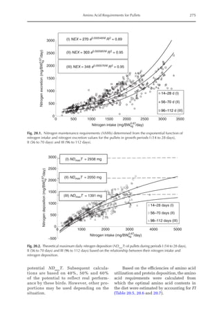
![Amino Acid Requirements for Pullets 273
Nitrogen maintenance requirement (NMR)
and maximum of theoretical potential
for nitrogen deposition (NDmax
T)
NMR (mg/BWkg
0.67
/day) was estimated by fit-
ting an exponential function of NI and NEX
(NEX = NMR·eb·NI
). NMR is the result of an ex-
trapolation when the NI is equal to zero; e is
the basic number of the natural logarithm;
and b is the equation parameter that repre-
sents the slope of the exponential function.Ni-
trogen retention (NR, mg/BWkg
0.67
/day) is the
sum of ND and NMR, and the theoretical max-
imum for daily nitrogen
retention (NRmax
T,
mg/BWkg
0.67
/day) is the threshold value of the
exponential function between NI and ND, i.e.:
NR = NRmax
T × (1 – e–b × NI
)
Or:
ND = NRmax
T × (1 – e–b × NI
) – NMR
Data obtained from the four trials were used
to determine NMR, NRmax
T, and NDmax
T, the
latter being calculated as the difference be-
tween NRmax
T and NMR. PDmax
T was calcu-
lated as NDmax
T × 6.25.
Because these parameters express the
theoretical potential for protein deposition
of the genotype studied, data from the four
trials were combined for further analysis.
Amino acid efficiency
The efficiencies of utilization of the test
amino acids (bc–1
) were calculated using
data from T2, T3 and T4, which involved
individual limiting amino acids according
to the following equation:
b = [ln NRmax
T – ln (NRmax
T – NR)]/NI
Where b is the slope of the exponential func-
tion resulting from graded amino acid or pro-
tein supply and indicates the dietary protein
quality independent of NI.
The amino acid intake needed for a
given NR is determined using the following
equation, as derived by transformation of
the basic function, with NI being replaced
by intake of the LAA:
LAAI = [ln NRmax
T – ln
(NRmax
T – NR)]/16 ·bc –1
Where LAAI is the daily intake of the limit-
ing amino acid (mg/BWkg
0.67
) needed for the
intended response level (NR); and bc–1
is the
linear slope resulting from the regression of
the concentration of the LAA (c = g amino
acid/100 g CP) in the feed protein on protein
quality b. The bc–1
considered was in the
linear range, where in each trial an amino
acid was limiting. The conversion factor for
NI based on the amino acid is given by the
equation NI = 16 LAAI/c.
Amino acid requirements
NRmax
T is the theoretical maximum or poten-
tial for nitrogen retention. In practice, it is
impossible for the birds to achieve this theor-
etical threshold. Consequently, graded pro-
portions of the potential (e.g. 40%, 50% and
60% of NDmax
T) were used to calculate the
Lys, Met and Thr requirements for pullets.
Statistical analysis
The Gauss method of the NLIN procedure in
SAS software (version 9.2) was used to esti-
mate the parameter values in the above
equations. This method considers the sum
of the least squares of the distances between
the model and each point.
Results
Nitrogen balance
We studied chickens of the Dekalb White
strain throughout the same growth periods
in each of the trials. Therefore, the results
for all of the nitrogen balance periods within
equal age periods are summarized in Table 20.3.
As the content of the limiting nutrient
increased, the values for the NI, NEX and
nitrogen balance (ND) also increased. Birds
fed L1 had lower feed intake and body
weight compared to those fed diets with
higher protein contents, and the values of
these variables were almost constant for the
latter birds.](https://image.slidesharecdn.com/nutritionalmodellingforpigsandpoultry-240127070709-ba59d9b4/85/Nutritional-modelling-for-pigs-and-poultry-pdf-288-320.jpg)
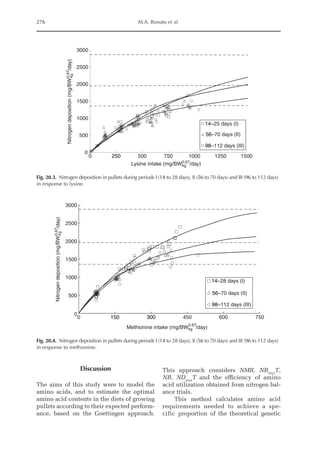
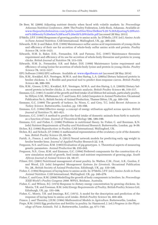
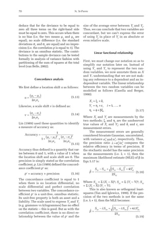
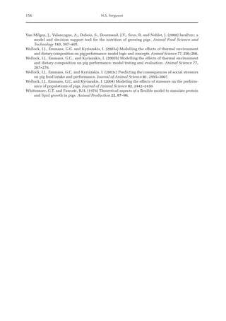
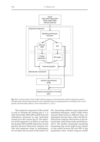
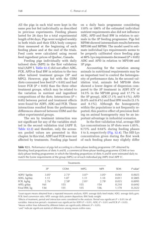
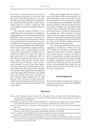
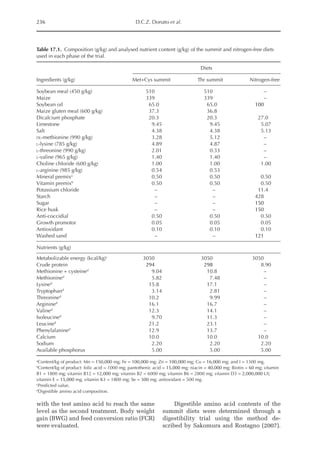
![Amino Acid Requirements for Pullets 277
potential for daily protein deposition.
Therefore, a description of the potential ni-
trogen deposition of various strains is indis-
pensable. As in other approaches for growth
studies, the increased deposition of nitro-
gen or protein with age was considered
here. Unlike other approaches, the descrip-
tion of nitrogen retention was separated
into two parts, the first being the NMR,
which is independent of nitrogen intake
and appears to be specific for each genotype,
and the second part is the physiological
response boundary for given nitrogen de-
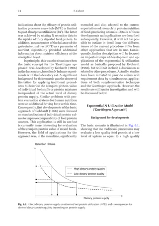
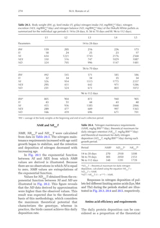
position rates.
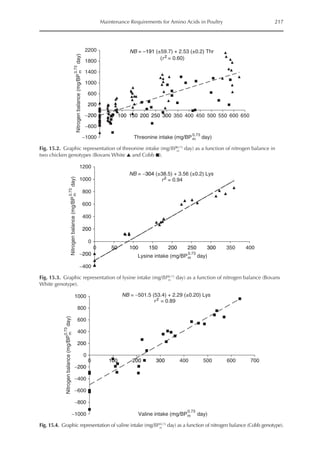
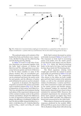
The average value for NMR, based on
the three growth phases studied, was 307
mg/BWkg
0.67
/day, with NMR being extrapo-
lated from NI = 0. The equivalent value for
3000
2500
2000
1500
1000
500
0
0 150 300 450 600 750
14–28 days (I)
56–70 days (II)
98–112 days (III)
Threonine intake (mg/BWkg /day)
0.67
Nitrogen
deposition
(mg/BW
kg
/day)
0.67
Fig. 20.5. Nitrogen deposition in pullets during periods I (14 to 28 days), II (56 to 70 days) and III (96 to 112
days) in response to threonine.
Table 20.5. Calculated amino acid requirements and optimal dietary contents of Lys, Met and Thr for pullets
during growth period I (14 to 28 days, mean BW = 222 g) depending on protein deposition (PD) and
observed amino acid efficiency.
Lys Met Thr
Efficiency of AA (bc–1
)a
50 170 100
PD (g/day)b
2.9 3.7 4.4 2.9 3.7 4.4 2.9 3.7 4.4
AA requirementc
mg/BWkg
0.67
/day 651 884 1168 190 257 340 304 413 546
mg/day (at mean BW) 238 322 426 69 94 124 111 151 199
Optimal dietary content (g/kg)d
9.50 12.9 17.1 2.77 3.75 4.96 4.44 6.03 7.96
a
Efficiency of amino acid utilization (bc–1
) considering that b = [ln NRmax
T – ln (NRmax
T – NR)]/NI and c = protein content of
the feed.
b
Protein deposition values at 40%, 50% and 60% of the theoretical maximum for the daily nitrogen deposition (NDmax
T).
c
Amino acid requirements were calculated using the equation LAAI = [ln NRmax
T – ln (NRmax
T – NR)]/16bc–1
.
d
For a daily feed intake of 25 g according to the pullet management guide.](https://image.slidesharecdn.com/nutritionalmodellingforpigsandpoultry-240127070709-ba59d9b4/85/Nutritional-modelling-for-pigs-and-poultry-pdf-292-320.jpg)
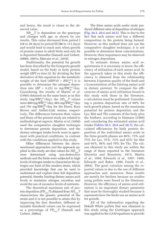
![278 M.A. Bonato et al.
laying hens determined by Filardi et al.
(2000) was 178 mg/BWkg
0.75
/day. Our values
were also higher than the 153 mg/BWkg
0.75
/
day for Passeriformes (Allen and Hume,
2001) and 171 mg/BWkg
0.67
/day for slow-
growing broilers (Samadi and Liebert, 2007b);
however, they were 18% higher than the
values determined for broilers (Samadi and
Liebert, 2006a).
According to Reeds and Lobley (1980),
when nitrogen is absent from the diet (NI = 0),
catabolism or degradation of body protein
occurs in order to maintain the pool of free
amino acids for protein synthesis according
to the metabolic priorities; the result of this
degradation process is quantified in the
NMR, so that differences found in NMR
values can be associated with protein syn-
thesis and degradation rates of different
genotypes.
According to the traditional method de-
scribed by Sakomura and Rostagno (2007)
NMR is determined by positive and nega-
tive NB responses. The negative balance is
limited by the rate of protein degradation,
which tends to increase endogenous losses
and hence NMR. Thus, with this approach,
the positive NB is used to determine NMR,
Table 20.7. Calculated amino acid requirements and optimal dietary contents of Lys, Met and Thr for pullets
during growth period III (96 to 112 days, mean BW = 920 g), depending on protein deposition (PD) and
observed amino acid efficiency.
Lys Met Thr
Efficiency of amino acid (bc–1
)a
100 350 180
PD (g/day)b
4.1 5.1 6.2 4.1 5.1 6.2 4.1 5.1 6.2
Amino acid requirementc
mg/BWkg
0.67
/day 309 419 554 91 123 162 177 240 318
mg/day (at mean BW) 292 397 524 86 116 154 167 227 300
Optimal dietary content (g/kg)4=d
4.00 5.43 7.18 1.51 2.05 2.71 2.10 2.85 3.76
a
Efficiency of amino acid utilization (bc–1
) considering that b = [ln NRmax
T – ln (NRmax
T – NR)]/NI and c = protein content of
the feed.
b
Protein deposition values at 40%, 50% and 60% of the theoretical maximum for the daily nitrogen deposition (NDmax
T).
c
Amino acid requirements were calculated using the equation LAAI = [ln NRmax
T – ln (NRmax
T – NR)]/16bc–1
.
d
Daily feed intake at 65 g according to the pullet management guide.
Table 20.6. Calculated amino acid requirements and optimal dietary contents of Lys, Met and Thr for pullets
during growth period II (56 to 70 days, mean BW = 582 g), depending on protein deposition (PD) and
observed amino acid efficiency.
Lys Met Thr
Efficiency of AA (bc–1
)a
90 230 160
PD (g/day)b
4.1 5.1 6.1 4.1 5.1 6.1 4.1 5.1 6.1
AA requirementc
mg/BWkg
0.67
/day 374 507 671 141 192 253 196 266 351
mg/day (at mean BW) 260 353 467 98 133 176 136 185 245
Optimal dietary content (g/kg)d
5.78 7.85 10.4 2.18 2.96 3.92 3.03 4.11 5.43
a
Efficiency of amino acid utilization (bc–1
) considering that b = [ln NRmax
T – ln (NRmax
T – NR)]/NI and c = protein content of
the feed.
b
Protein deposition values at 40%, 50% and 60% of the theoretical maximum for the daily nitrogen deposition (NDmax
T).
c
Amino acid requirements were calculated using the equation LAAI = [ln NRmax
T – ln (NRmax
T – NR)]/16bc–1
.
d
For a daily feed intake of 45 g according to the pullet management guide.](https://image.slidesharecdn.com/nutritionalmodellingforpigsandpoultry-240127070709-ba59d9b4/85/Nutritional-modelling-for-pigs-and-poultry-pdf-293-320.jpg)

The document is a compilation of papers presented at the International Symposium of Modelling in Pig and Poultry Production, held in June 2013 in Brazil, addressing nutritional modeling in these sectors. It aims to enhance the application of modeling techniques among Brazilian academics and agro-businesses, covering various aspects, including nutrient utilization and growth predictions. Key contributors include researchers and experts from institutions like Universidade Estadual Paulista and the University of Kwazulu-Natal.


![OSTA TRAINING-introduction [Autosaved].pptx](https://cdn.slidesharecdn.com/ss_thumbnails/ostatraining-introductionautosaved-240507111126-2f0d1553-thumbnail.jpg?width=640&height=640&fit=bounds)


