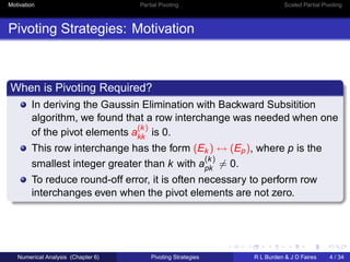
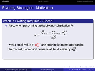
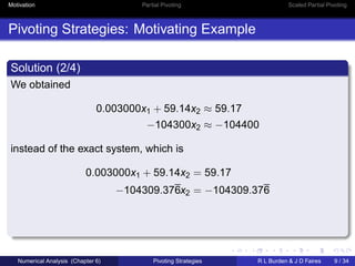
Direct Methods for Solving Linear Systems
Pivoting Strategies
Numerical Analysis (9th Edition)
R L Burden & J D Faires
Beamer Presentation Slides
prepared by
John Carroll
Dublin City University
c 2011 Brooks/Cole, Cengage Learning
Motivation Partial Pivoting Scaled Partial Pivoting
Outline
1 Why Pivoting May be Necessary
Numerical Analysis (Chapter 6) Pivoting Strategies R L Burden & J D Faires 2 / 34
Motivation Partial Pivoting Scaled Partial Pivoting
Outline
1 Why Pivoting May be Necessary
2 Gaussian Elimination with Partial Pivoting
Numerical Analysis (Chapter 6) Pivoting Strategies R L Burden & J D Faires 2 / 34
Motivation Partial Pivoting Scaled Partial Pivoting
Outline
1 Why Pivoting May be Necessary
2 Gaussian Elimination with Partial Pivoting
3 Gaussian Elimination with Scaled Partial (Scaled-Column) Pivoting
Numerical Analysis (Chapter 6) Pivoting Strategies R L Burden & J D Faires 2 / 34
Motivation Partial Pivoting Scaled Partial Pivoting
Outline
1 Why Pivoting May be Necessary
2 Gaussian Elimination with Partial Pivoting
3 Gaussian Elimination with Scaled Partial (Scaled-Column) Pivoting
Numerical Analysis (Chapter 6) Pivoting Strategies R L Burden & J D Faires 3 / 34
Motivation Partial Pivoting Scaled Partial Pivoting
Pivoting Strategies: Motivation
When is Pivoting Required?
Numerical Analysis (Chapter 6) Pivoting Strategies R L Burden & J D Faires 4 / 34
Motivation Partial Pivoting Scaled Partial Pivoting
Pivoting Strategies: Motivation
When is Pivoting Required?
In deriving the Gaussin Elimination with Backward Subsitition
algorithm, we found that a row interchange was needed when one
of the pivot elements a
(k)
kk is 0.
This row interchange has the form (Ek ) ↔ (Ep), where p is the
smallest integer greater than k with a
(k)
pk 6= 0.
To reduce round-off error, it is often necessary to perform row
interchanges even when the pivot elements are not zero.
Numerical Analysis (Chapter 6) Pivoting Strategies R L Burden & J D Faires 4 / 34
Motivation Partial Pivoting Scaled Partial Pivoting
Pivoting Strategies: Motivation
When is Pivoting Required? (Cont’d)
If a
(k)
kk is small in magnitude compared to a
(k)
jk , then the magnitude
of the multiplier
mjk =
a
(k)
jk
a
(k)
kk
will be much larger than 1.
Numerical Analysis (Chapter 6) Pivoting Strategies R L Burden & J D Faires 5 / 34
Motivation Partial Pivoting Scaled Partial Pivoting
Pivoting Strategies: Motivation
When is Pivoting Required? (Cont’d)
If a
(k)
kk is small in magnitude compared to a
(k)
jk , then the magnitude
of the multiplier
mjk =
a
(k)
jk
a
(k)
kk
will be much larger than 1.
Round-off error introduced in the computation of one of the terms
a
(k)
kl is multiplied by mjk when computing a
(k+1)
jl , which compounds
the original error.
Numerical Analysis (Chapter 6) Pivoting Strategies R L Burden & J D Faires 5 / 34
Motivation Partial Pivoting Scaled Partial Pivoting
Pivoting Strategies: Motivation
When is Pivoting Required? (Cont’d)
Also, when performing the backward substitution for
xk =
a
(k)
k,n+1 −
Pn
j=k+1 a
(k)
kj
a
(k)
kk
with a small value of a
(k)
kk , any error in the numerator can be
dramatically increased because of the division by a
(k)
kk .
Numerical Analysis (Chapter 6) Pivoting Strategies R L Burden & J D Faires 6 / 34
Motivation Partial Pivoting Scaled Partial Pivoting
Pivoting Strategies: Motivation
When is Pivoting Required? (Cont’d)
Also, when performing the backward substitution for
xk =
a
(k)
k,n+1 −
Pn
j=k+1 a
(k)
kj
a
(k)
kk
with a small value of a
(k)
kk , any error in the numerator can be
dramatically increased because of the division by a
(k)
kk .
The following example will show that even for small systems,
round-off error can dominate the calculations.
Numerical Analysis (Chapter 6) Pivoting Strategies R L Burden & J D Faires 6 / 34
Motivation Partial Pivoting Scaled Partial Pivoting
Pivoting Strategies: Motivation
Example
Apply Gaussian elimination to the system
E1 : 0.003000x1 + 59.14x2 = 59.17
E2 : 5.291x1 − 6.130x2 = 46.78
using four-digit arithmetic with rounding, and compare the results to
the exact solution x1 = 10.00 and x2 = 1.000.
Numerical Analysis (Chapter 6) Pivoting Strategies R L Burden & J D Faires 7 / 34
Motivation Partial Pivoting Scaled Partial Pivoting
Pivoting Strategies: Motivating Example
Solution (1/4)
The first pivot element, a
(1)
11 = 0.003000, is small, and its
associated multiplier,
m21 =
5.291
0.003000
= 1763.66
rounds to the large number 1764.
Numerical Analysis (Chapter 6) Pivoting Strategies R L Burden & J D Faires 8 / 34
Motivation Partial Pivoting Scaled Partial Pivoting
Pivoting Strategies: Motivating Example
Solution (1/4)
The first pivot element, a
(1)
11 = 0.003000, is small, and its
associated multiplier,
m21 =
5.291
0.003000
= 1763.66
rounds to the large number 1764.
Performing (E2 − m21E1) → (E2) and the appropriate rounding
gives the system
0.003000x1 + 59.14x2 ≈ 59.17
−104300x2 ≈ −104400
Numerical Analysis (Chapter 6) Pivoting Strategies R L Burden & J D Faires 8 / 34
Motivation Partial Pivoting Scaled Partial Pivoting
Pivoting Strategies: Motivating Example
Solution (2/4)
We obtained
0.003000x1 + 59.14x2 ≈ 59.17
−104300x2 ≈ −104400
Numerical Analysis (Chapter 6) Pivoting Strategies R L Burden & J D Faires 9 / 34
Motivation Partial Pivoting Scaled Partial Pivoting
Pivoting Strategies: Motivating Example
Solution (2/4)
We obtained
0.003000x1 + 59.14x2 ≈ 59.17
−104300x2 ≈ −104400
instead of the exact system, which is
0.003000x1 + 59.14x2 = 59.17
−104309.376x2 = −104309.376
The disparity in the magnitudes of m21a13 and a23 has introduced
round-off error, but the round-off error has not yet been propagated.
Numerical Analysis (Chapter 6) Pivoting Strategies R L Burden & J D Faires 9 / 34
Motivation Partial Pivoting Scaled Partial Pivoting
Pivoting Strategies: Motivating Example
Solution (3/4)
Backward substitution yields
x2 ≈ 1.001
which is a close approximation to the actual value, x2 = 1.000.
Numerical Analysis (Chapter 6) Pivoting Strategies R L Burden & J D Faires 10 / 34
Motivation Partial Pivoting Scaled Partial Pivoting
Pivoting Strategies: Motivating Example
Solution (3/4)
Backward substitution yields
x2 ≈ 1.001
which is a close approximation to the actual value, x2 = 1.000.
However, because of the small pivot a11 = 0.003000,
x1 ≈
59.17 − (59.14)(1.001)
0.003000
= −10.00
contains the small error of 0.001 multiplied by
59.14
0.003000
≈ 20000
This ruins the approximation to the actual value x1 = 10.00.
Numerical Analysis (Chapter 6) Pivoting Strategies R L Burden & J D Faires 10 / 34
Motivation Partial Pivoting Scaled Partial Pivoting
Pivoting Strategies: Motivating Example
Solution (4/4)
This is clearly a contrived example and the graph shows why the error
can so easily occur.
x1
E1
E2
10
210
Approximation
(210, 1.001) Exact solution
(10, 1)
x2
For larger systems it is much more difficult to predict in advance when
devastating round-off error might occur.
Numerical Analysis (Chapter 6) Pivoting Strategies R L Burden & J D Faires 11 / 34
Motivation Partial Pivoting Scaled Partial Pivoting
Outline
1 Why Pivoting May be Necessary
2 Gaussian Elimination with Partial Pivoting
3 Gaussian Elimination with Scaled Partial (Scaled-Column) Pivoting
Numerical Analysis (Chapter 6) Pivoting Strategies R L Burden & J D Faires 12 / 34
Motivation Partial Pivoting Scaled Partial Pivoting
Gaussian Elimination with Partial Pivoting
Meeting a small pivot element
Numerical Analysis (Chapter 6) Pivoting Strategies R L Burden & J D Faires 13 / 34
Motivation Partial Pivoting Scaled Partial Pivoting
Gaussian Elimination with Partial Pivoting
Meeting a small pivot element
The last example shows how difficulties can arise when the pivot
element a
(k)
kk is small relative to the entries a
(k)
ij , for k ≤ i ≤ n and
k ≤ j ≤ n.
To avoid this problem, pivoting is performed by selecting an
element a
(k)
pq with a larger magnitude as the pivot, and
interchanging the kth and pth rows.
This can be followed by the interchange of the kth and qth
columns, if necessary.
Numerical Analysis (Chapter 6) Pivoting Strategies R L Burden & J D Faires 13 / 34
Motivation Partial Pivoting Scaled Partial Pivoting
Gaussian Elimination with Partial Pivoting
The Partial Pivoting Strategy
Numerical Analysis (Chapter 6) Pivoting Strategies R L Burden & J D Faires 14 / 34
Motivation Partial Pivoting Scaled Partial Pivoting
Gaussian Elimination with Partial Pivoting
The Partial Pivoting Strategy
The simplest strategy is to select an element in the same column
that is below the diagonal and has the largest absolute value;
specifically, we determine the smallest p ≥ k such that
a
(k)
pk = max
k≤i≤n
|a
(k)
ik |
and perform (Ek ) ↔ (Ep).
In this case no interchange of columns is used.
Numerical Analysis (Chapter 6) Pivoting Strategies R L Burden & J D Faires 14 / 34
Motivation Partial Pivoting Scaled Partial Pivoting
Gaussian Elimination with Partial Pivoting
Example
Apply Gaussian elimination to the system
E1 : 0.003000x1 + 59.14x2 = 59.17
E2 : 5.291x1 − 6.130x2 = 46.78
using partial pivoting and 4-digit arithmetic with rounding, and compare
the results to the exact solution x1 = 10.00 and x2 = 1.000.
Numerical Analysis (Chapter 6) Pivoting Strategies R L Burden & J D Faires 15 / 34
Motivation Partial Pivoting Scaled Partial Pivoting
Gaussian Elimination with Partial Pivoting
E1 : 0.003000x1 + 59.14x2 = 59.17
E2 : 5.291x1 − 6.130x2 = 46.78
Solution (1/3)
Numerical Analysis (Chapter 6) Pivoting Strategies R L Burden & J D Faires 16 / 34
Motivation Partial Pivoting Scaled Partial Pivoting
Gaussian Elimination with Partial Pivoting
E1 : 0.003000x1 + 59.14x2 = 59.17
E2 : 5.291x1 − 6.130x2 = 46.78
Solution (1/3)
The partial-pivoting procedure first requires finding
max
n
|a
(1)
11 |, |a
(1)
21 |
o
= max {|0.003000|, |5.291|} = |5.291| = |a
(1)
21 |
This requires that the operation (E2) ↔ (E1) be performed to produce
the equivalent system
E1 : 5.291x1 − 6.130x2 = 46.78,
E2 : 0.003000x1 + 59.14x2 = 59.17
Numerical Analysis (Chapter 6) Pivoting Strategies R L Burden & J D Faires 16 / 34
Motivation Partial Pivoting Scaled Partial Pivoting
Gaussian Elimination with Partial Pivoting
E1 : 5.291x1 − 6.130x2 = 46.78,
E2 : 0.003000x1 + 59.14x2 = 59.17
Solution (2/3)
Numerical Analysis (Chapter 6) Pivoting Strategies R L Burden & J D Faires 17 / 34
Motivation Partial Pivoting Scaled Partial Pivoting
Gaussian Elimination with Partial Pivoting
E1 : 5.291x1 − 6.130x2 = 46.78,
E2 : 0.003000x1 + 59.14x2 = 59.17
Solution (2/3)
The multiplier for this system is
m21 =
a
(1)
21
a
(1)
11
= 0.0005670
and the operation (E2 − m21E1) → (E2) reduces the system to
5.291x1 − 6.130x2 ≈ 46.78
59.14x2 ≈ 59.14
Numerical Analysis (Chapter 6) Pivoting Strategies R L Burden & J D Faires 17 / 34
Motivation Partial Pivoting Scaled Partial Pivoting
Gaussian Elimination with Partial Pivoting
5.291x1 − 6.130x2 ≈ 46.78
59.14x2 ≈ 59.14
Solution (3/3)
Numerical Analysis (Chapter 6) Pivoting Strategies R L Burden & J D Faires 18 / 34
Motivation Partial Pivoting Scaled Partial Pivoting
Gaussian Elimination with Partial Pivoting
5.291x1 − 6.130x2 ≈ 46.78
59.14x2 ≈ 59.14
Solution (3/3)
The 4-digit answers resulting from the backward substitution are the
correct values
x1 = 10.00 and x2 = 1.000
Numerical Analysis (Chapter 6) Pivoting Strategies R L Burden & J D Faires 18 / 34
Motivation Partial Pivoting Scaled Partial Pivoting
Gaussian Elimination/Partial Pivoting Algorithm (1/4)
To solve the n × n linear system
E1 : a11x1 + a12x2 + · · · + a1nxn = a1,n+1
E2 : a21x1 + a22x2 + · · · + a2nxn = a2,n+1
.
.
.
.
.
.
En : an1x1 + an2x2 + · · · + annxn = an,n+1
Numerical Analysis (Chapter 6) Pivoting Strategies R L Burden & J D Faires 19 / 34
Motivation Partial Pivoting Scaled Partial Pivoting
Gaussian Elimination/Partial Pivoting Algorithm (1/4)
To solve the n × n linear system
E1 : a11x1 + a12x2 + · · · + a1nxn = a1,n+1
E2 : a21x1 + a22x2 + · · · + a2nxn = a2,n+1
.
.
.
.
.
.
En : an1x1 + an2x2 + · · · + annxn = an,n+1
INPUT number of unknowns and equations n; augmented
matrix A = [aij] where 1 ≤ i ≤ n and 1 ≤ j ≤ n + 1.
OUTPUT solution x1, . . . , xn or message that the linear
system has no unique solution.
Numerical Analysis (Chapter 6) Pivoting Strategies R L Burden & J D Faires 19 / 34
Motivation Partial Pivoting Scaled Partial Pivoting
Gaussian Elimination/Partial Pivoting Algorithm (2/4)
Step 1 For i = 1, . . . , n set NROW(i) = i (Initialize row pointer)
Step 2 For i = 1, . . . , n − 1 do Steps 3–6 (Elimination process)
Numerical Analysis (Chapter 6) Pivoting Strategies R L Burden & J D Faires 20 / 34
Motivation Partial Pivoting Scaled Partial Pivoting
Gaussian Elimination/Partial Pivoting Algorithm (2/4)
Step 1 For i = 1, . . . , n set NROW(i) = i (Initialize row pointer)
Step 2 For i = 1, . . . , n − 1 do Steps 3–6 (Elimination process)
Step 3 Let p be the smallest integer with i ≤ p ≤ n and
|a(NROW(p), i)| = maxi≤j≤n |a(NROW(j), i)|
(Notation: a(NROW(i), j) ≡ aNROWi ,j)
Step 4 If a(NROW(p), i) = 0 then
OUTPUT(‘no unique solution exists’)
STOP
Step 5 If NROW(i) 6= NROW(p) then set NCOPY = NROW(i)
NROW(i) = NROW(p)
NROW(p) = NCOPY
(Simulated row interchange)
Numerical Analysis (Chapter 6) Pivoting Strategies R L Burden & J D Faires 20 / 34
Motivation Partial Pivoting Scaled Partial Pivoting
Gaussian Elimination/Partial Pivoting Algorithm (3/4)
Step 6 For j = i + 1, . . . , n do Steps 7 & 8
Numerical Analysis (Chapter 6) Pivoting Strategies R L Burden & J D Faires 21 / 34
Motivation Partial Pivoting Scaled Partial Pivoting
Gaussian Elimination/Partial Pivoting Algorithm (3/4)
Step 6 For j = i + 1, . . . , n do Steps 7 & 8
Step 7 Set
m(NROW(j), i) = a(NROW(j), i)/a(NROW(i), i)
Numerical Analysis (Chapter 6) Pivoting Strategies R L Burden & J D Faires 21 / 34
Motivation Partial Pivoting Scaled Partial Pivoting
Gaussian Elimination/Partial Pivoting Algorithm (3/4)
Step 6 For j = i + 1, . . . , n do Steps 7 & 8
Step 7 Set
m(NROW(j), i) = a(NROW(j), i)/a(NROW(i), i)
Step 8 Perform
(ENROW(j) − m(NROW(j), i) · ENROW(i)) → (ENROW(j))
Step 9 If a(NROW(n), n) = 0 then
OUTPUT(‘no unique solution exists’)
STOP
Numerical Analysis (Chapter 6) Pivoting Strategies R L Burden & J D Faires 21 / 34
Motivation Partial Pivoting Scaled Partial Pivoting
Gaussian Elimination/Partial Pivoting Algorithm (4/4)
Step 10 Set xn = a(NROW(n), n + 1)/a(NROW(n), n)
(Start backward substitution)
Numerical Analysis (Chapter 6) Pivoting Strategies R L Burden & J D Faires 22 / 34
Motivation Partial Pivoting Scaled Partial Pivoting
Gaussian Elimination/Partial Pivoting Algorithm (4/4)
Step 10 Set xn = a(NROW(n), n + 1)/a(NROW(n), n)
(Start backward substitution)
Step 11 For i = n − 1, . . . , 1
set xi =
a(NROW(i), n + 1) −
Pn
j=i+1 a(NROW(i), j) · xj
a(NROW(i), i)
Step 12 OUTPUT (x1, . . . , xn) (Procedure completed successfully)
STOP
Numerical Analysis (Chapter 6) Pivoting Strategies R L Burden & J D Faires 22 / 34
Motivation Partial Pivoting Scaled Partial Pivoting
Gaussian Elimination with Partial Pivoting
Can Partial Pivoting fail?
Numerical Analysis (Chapter 6) Pivoting Strategies R L Burden & J D Faires 23 / 34
Motivation Partial Pivoting Scaled Partial Pivoting
Gaussian Elimination with Partial Pivoting
Can Partial Pivoting fail?
Each multiplier mji in the partial pivoting algorithm has magnitude
less than or equal to 1.
Numerical Analysis (Chapter 6) Pivoting Strategies R L Burden & J D Faires 23 / 34
Motivation Partial Pivoting Scaled Partial Pivoting
Gaussian Elimination with Partial Pivoting
Can Partial Pivoting fail?
Each multiplier mji in the partial pivoting algorithm has magnitude
less than or equal to 1.
Although this strategy is sufficient for many linear systems,
situations do arise when it is inadequate.
The following (contrived) example illusrates the point.
Numerical Analysis (Chapter 6) Pivoting Strategies R L Burden & J D Faires 23 / 34
Motivation Partial Pivoting Scaled Partial Pivoting
Gaussian Elimination with Partial Pivoting
Example: When Partial Pivoting Fails
The linear system
E1 : 30.00x1 + 591400x2 = 591700
E2 : 5.291x1 − 6.130x2 = 46.78
is the same as that in the two previous examples except that all the
entries in the first equation have been multiplied by 104.
Numerical Analysis (Chapter 6) Pivoting Strategies R L Burden & J D Faires 24 / 34
Motivation Partial Pivoting Scaled Partial Pivoting
Gaussian Elimination with Partial Pivoting
Example: When Partial Pivoting Fails
The linear system
E1 : 30.00x1 + 591400x2 = 591700
E2 : 5.291x1 − 6.130x2 = 46.78
is the same as that in the two previous examples except that all the
entries in the first equation have been multiplied by 104.
The partial pivoting procedure described in the algorithm with 4-digit
arithmetic leads to the same incorrect results as obtained in the first
example (Gaussian elimination without pivoting).
Numerical Analysis (Chapter 6) Pivoting Strategies R L Burden & J D Faires 24 / 34
Motivation Partial Pivoting Scaled Partial Pivoting
Gaussian Elimination with Partial Pivoting
E1 : 30.00x1 + 591400x2 = 591700
E2 : 5.291x1 − 6.130x2 = 46.78
Apply Partial Pivoting
Numerical Analysis (Chapter 6) Pivoting Strategies R L Burden & J D Faires 25 / 34
Motivation Partial Pivoting Scaled Partial Pivoting
Gaussian Elimination with Partial Pivoting
E1 : 30.00x1 + 591400x2 = 591700
E2 : 5.291x1 − 6.130x2 = 46.78
Apply Partial Pivoting
The maximal value in the first column is 30.00, and the multiplier
m21 =
5.291
30.00
= 0.1764
leads to the system
30.00x1 + 591400x2 ≈ 591700
−104300x2 ≈ −104400
which has the same inaccurate solutions as in the first example:
x2 ≈ 1.001 and x1 ≈ −10.00.
Numerical Analysis (Chapter 6) Pivoting Strategies R L Burden & J D Faires 25 / 34
Motivation Partial Pivoting Scaled Partial Pivoting
Outline
1 Why Pivoting May be Necessary
2 Gaussian Elimination with Partial Pivoting
3 Gaussian Elimination with Scaled Partial (Scaled-Column) Pivoting
Numerical Analysis (Chapter 6) Pivoting Strategies R L Burden & J D Faires 26 / 34
Motivation Partial Pivoting Scaled Partial Pivoting
Gaussian Elimination with Scaled Partial Pivoting
Scaled Partial Pivoting
Numerical Analysis (Chapter 6) Pivoting Strategies R L Burden & J D Faires 27 / 34
Motivation Partial Pivoting Scaled Partial Pivoting
Gaussian Elimination with Scaled Partial Pivoting
Scaled Partial Pivoting
Scaled partial pivoting places the element in the pivot position that
is largest relative to the entries in its row.
The first step in this procedure is to define a scale factor si for
each row as
si = max
1≤j≤n
aij
If we have si = 0 for some i, then the system has no unique
solution since all entries in the ith row are 0.
Numerical Analysis (Chapter 6) Pivoting Strategies R L Burden & J D Faires 27 / 34
Motivation Partial Pivoting Scaled Partial Pivoting
Gaussian Elimination with Scaled Partial Pivoting
Scaled Partial Pivoting (Cont’d)
Assuming that this is not the case, the appropriate row
interchange to place zeros in the first column is determined by
choosing the least integer p with
|ap1|
sp
= max
1≤k≤n
|ak1|
sk
and performing (E1) ↔ (Ep).
Numerical Analysis (Chapter 6) Pivoting Strategies R L Burden & J D Faires 28 / 34
Motivation Partial Pivoting Scaled Partial Pivoting
Gaussian Elimination with Scaled Partial Pivoting
Scaled Partial Pivoting (Cont’d)
Assuming that this is not the case, the appropriate row
interchange to place zeros in the first column is determined by
choosing the least integer p with
|ap1|
sp
= max
1≤k≤n
|ak1|
sk
and performing (E1) ↔ (Ep).
The effect of scaling is to ensure that the largest element in each
row has a relative magnitude of 1 before the comparison for row
interchange is performed.
Numerical Analysis (Chapter 6) Pivoting Strategies R L Burden & J D Faires 28 / 34
Motivation Partial Pivoting Scaled Partial Pivoting
Gaussian Elimination with Scaled Partial Pivoting
Scaled Partial Pivoting (Cont’d)
In a similar manner, before eliminating the variable xi using the
operations
Ek − mkiEi , for k = i + 1, . . . , n,
we select the smallest integer p ≥ i with
|api|
sp
= max
i≤k≤n
|aki|
sk
and perform the row interchange (Ei) ↔ (Ep) if i 6= p.
Numerical Analysis (Chapter 6) Pivoting Strategies R L Burden & J D Faires 29 / 34
Motivation Partial Pivoting Scaled Partial Pivoting
Gaussian Elimination with Scaled Partial Pivoting
Scaled Partial Pivoting (Cont’d)
In a similar manner, before eliminating the variable xi using the
operations
Ek − mkiEi , for k = i + 1, . . . , n,
we select the smallest integer p ≥ i with
|api|
sp
= max
i≤k≤n
|aki|
sk
and perform the row interchange (Ei) ↔ (Ep) if i 6= p.
The scale factors s1, . . . , sn are computed only once, at the start
of the procedure.
They are row dependent, so they must also be interchanged when
row interchanges are performed.
Numerical Analysis (Chapter 6) Pivoting Strategies R L Burden & J D Faires 29 / 34
Motivation Partial Pivoting Scaled Partial Pivoting
Gaussian Elimination with Scaled Partial Pivoting
Example
Returning to the previous ewxample, we will appl scaled partial
pivoting for the linear system:
E1 : 30.00x1 + 591400x2 = 591700
E2 : 5.291x1 − 6.130x2 = 46.78
Numerical Analysis (Chapter 6) Pivoting Strategies R L Burden & J D Faires 30 / 34
Motivation Partial Pivoting Scaled Partial Pivoting
Gaussian Elimination with Scaled Partial Pivoting
E1 : 30.00x1 + 591400x2 = 591700
E2 : 5.291x1 − 6.130x2 = 46.78
Solution (1/2)
Numerical Analysis (Chapter 6) Pivoting Strategies R L Burden & J D Faires 31 / 34
Motivation Partial Pivoting Scaled Partial Pivoting
Gaussian Elimination with Scaled Partial Pivoting
E1 : 30.00x1 + 591400x2 = 591700
E2 : 5.291x1 − 6.130x2 = 46.78
Solution (1/2)
We compute
s1 = max{|30.00|, |591400|} = 591400
and s2 = max{|5.291|, |−6.130|} = 6.130
so that
|a11|
s1
=
30.00
591400
= 0.5073 × 10⁻⁴
,
|a21|
s2
=
5.291
6.130
= 0.8631,
and the interchange (E1) ↔ (E2) is made.
Numerical Analysis (Chapter 6) Pivoting Strategies R L Burden & J D Faires 31 / 34
Motivation Partial Pivoting Scaled Partial Pivoting
Gaussian Elimination with Scaled Partial Pivoting
Solution (2/2)
Applying Gaussian elimination to the new system
5.291x1 − 6.130x2 = 46.78
30.00x1 + 591400x2 = 591700
produces the correct results: x1 = 10.00 and x2 = 1.000.
Numerical Analysis (Chapter 6) Pivoting Strategies R L Burden & J D Faires 32 / 34
Motivation Partial Pivoting Scaled Partial Pivoting
Gaussian Elimination/Scaled Partial Pivoting Algorithm
The only steps in this algorithm that differ from those of the Gaussian
Elimination with Scaled Partial Pivoting Algorithm are:
Numerical Analysis (Chapter 6) Pivoting Strategies R L Burden & J D Faires 33 / 34
Motivation Partial Pivoting Scaled Partial Pivoting
Gaussian Elimination/Scaled Partial Pivoting Algorithm
The only steps in this algorithm that differ from those of the Gaussian
Elimination with Scaled Partial Pivoting Algorithm are:
Step 1 For i = 1, . . . , n set si = max1≤j≤n |aij|
if si = 0 then OUTPUT (‘no unique solution exists’)
STOP
else set NROW(i) = i
Step 2 For i = 1, . . . , n − 1 do Steps 3–6 (Elimination process)
Step 3 Let p be the smallest integer with i ≤ p ≤ n and
|a(NROW(p), i)|
s(NROW(p))
= max
i≤j≤n
|a(NROW(j), i)|
s(NROW(j))
Numerical Analysis (Chapter 6) Pivoting Strategies R L Burden & J D Faires 33 / 34
Questions?

Numerical Method Pivoting Problems solving

  • 1.
    Direct Methods forSolving Linear Systems Pivoting Strategies Numerical Analysis (9th Edition) R L Burden & J D Faires Beamer Presentation Slides prepared by John Carroll Dublin City University c 2011 Brooks/Cole, Cengage Learning
  • 2.
    Motivation Partial PivotingScaled Partial Pivoting Outline 1 Why Pivoting May be Necessary Numerical Analysis (Chapter 6) Pivoting Strategies R L Burden & J D Faires 2 / 34
  • 3.
    Motivation Partial PivotingScaled Partial Pivoting Outline 1 Why Pivoting May be Necessary 2 Gaussian Elimination with Partial Pivoting Numerical Analysis (Chapter 6) Pivoting Strategies R L Burden & J D Faires 2 / 34
  • 4.
    Motivation Partial PivotingScaled Partial Pivoting Outline 1 Why Pivoting May be Necessary 2 Gaussian Elimination with Partial Pivoting 3 Gaussian Elimination with Scaled Partial (Scaled-Column) Pivoting Numerical Analysis (Chapter 6) Pivoting Strategies R L Burden & J D Faires 2 / 34
  • 5.
    Motivation Partial PivotingScaled Partial Pivoting Outline 1 Why Pivoting May be Necessary 2 Gaussian Elimination with Partial Pivoting 3 Gaussian Elimination with Scaled Partial (Scaled-Column) Pivoting Numerical Analysis (Chapter 6) Pivoting Strategies R L Burden & J D Faires 3 / 34
  • 6.
    Motivation Partial PivotingScaled Partial Pivoting Pivoting Strategies: Motivation When is Pivoting Required? Numerical Analysis (Chapter 6) Pivoting Strategies R L Burden & J D Faires 4 / 34
  • 7.
    Motivation Partial PivotingScaled Partial Pivoting Pivoting Strategies: Motivation When is Pivoting Required? In deriving the Gaussin Elimination with Backward Subsitition algorithm, we found that a row interchange was needed when one of the pivot elements a (k) kk is 0. Numerical Analysis (Chapter 6) Pivoting Strategies R L Burden & J D Faires 4 / 34
  • 8.
    Motivation Partial PivotingScaled Partial Pivoting Pivoting Strategies: Motivation When is Pivoting Required? In deriving the Gaussin Elimination with Backward Subsitition algorithm, we found that a row interchange was needed when one of the pivot elements a (k) kk is 0. This row interchange has the form (Ek ) ↔ (Ep), where p is the smallest integer greater than k with a (k) pk 6= 0. Numerical Analysis (Chapter 6) Pivoting Strategies R L Burden & J D Faires 4 / 34
  • 9.
    Motivation Partial PivotingScaled Partial Pivoting Pivoting Strategies: Motivation When is Pivoting Required? In deriving the Gaussin Elimination with Backward Subsitition algorithm, we found that a row interchange was needed when one of the pivot elements a (k) kk is 0. This row interchange has the form (Ek ) ↔ (Ep), where p is the smallest integer greater than k with a (k) pk 6= 0. To reduce round-off error, it is often necessary to perform row interchanges even when the pivot elements are not zero. Numerical Analysis (Chapter 6) Pivoting Strategies R L Burden & J D Faires 4 / 34
  • 10.
    Motivation Partial PivotingScaled Partial Pivoting Pivoting Strategies: Motivation When is Pivoting Required? (Cont’d) If a (k) kk is small in magnitude compared to a (k) jk , then the magnitude of the multiplier mjk = a (k) jk a (k) kk will be much larger than 1. Numerical Analysis (Chapter 6) Pivoting Strategies R L Burden & J D Faires 5 / 34
  • 11.
    Motivation Partial PivotingScaled Partial Pivoting Pivoting Strategies: Motivation When is Pivoting Required? (Cont’d) If a (k) kk is small in magnitude compared to a (k) jk , then the magnitude of the multiplier mjk = a (k) jk a (k) kk will be much larger than 1. Round-off error introduced in the computation of one of the terms a (k) kl is multiplied by mjk when computing a (k+1) jl , which compounds the original error. Numerical Analysis (Chapter 6) Pivoting Strategies R L Burden & J D Faires 5 / 34
  • 12.
    Motivation Partial PivotingScaled Partial Pivoting Pivoting Strategies: Motivation When is Pivoting Required? (Cont’d) Also, when performing the backward substitution for xk = a (k) k,n+1 − Pn j=k+1 a (k) kj a (k) kk with a small value of a (k) kk , any error in the numerator can be dramatically increased because of the division by a (k) kk . Numerical Analysis (Chapter 6) Pivoting Strategies R L Burden & J D Faires 6 / 34
  • 13.
    Motivation Partial PivotingScaled Partial Pivoting Pivoting Strategies: Motivation When is Pivoting Required? (Cont’d) Also, when performing the backward substitution for xk = a (k) k,n+1 − Pn j=k+1 a (k) kj a (k) kk with a small value of a (k) kk , any error in the numerator can be dramatically increased because of the division by a (k) kk . The following example will show that even for small systems, round-off error can dominate the calculations. Numerical Analysis (Chapter 6) Pivoting Strategies R L Burden & J D Faires 6 / 34
  • 14.
    Motivation Partial PivotingScaled Partial Pivoting Pivoting Strategies: Motivation Example Apply Gaussian elimination to the system E1 : 0.003000x1 + 59.14x2 = 59.17 E2 : 5.291x1 − 6.130x2 = 46.78 using four-digit arithmetic with rounding, and compare the results to the exact solution x1 = 10.00 and x2 = 1.000. Numerical Analysis (Chapter 6) Pivoting Strategies R L Burden & J D Faires 7 / 34
  • 15.
    Motivation Partial PivotingScaled Partial Pivoting Pivoting Strategies: Motivating Example Solution (1/4) The first pivot element, a (1) 11 = 0.003000, is small, and its associated multiplier, m21 = 5.291 0.003000 = 1763.66 rounds to the large number 1764. Numerical Analysis (Chapter 6) Pivoting Strategies R L Burden & J D Faires 8 / 34
  • 16.
    Motivation Partial PivotingScaled Partial Pivoting Pivoting Strategies: Motivating Example Solution (1/4) The first pivot element, a (1) 11 = 0.003000, is small, and its associated multiplier, m21 = 5.291 0.003000 = 1763.66 rounds to the large number 1764. Performing (E2 − m21E1) → (E2) and the appropriate rounding gives the system 0.003000x1 + 59.14x2 ≈ 59.17 −104300x2 ≈ −104400 Numerical Analysis (Chapter 6) Pivoting Strategies R L Burden & J D Faires 8 / 34
  • 17.
    Motivation Partial PivotingScaled Partial Pivoting Pivoting Strategies: Motivating Example Solution (2/4) We obtained 0.003000x1 + 59.14x2 ≈ 59.17 −104300x2 ≈ −104400 Numerical Analysis (Chapter 6) Pivoting Strategies R L Burden & J D Faires 9 / 34
  • 18.
    Motivation Partial PivotingScaled Partial Pivoting Pivoting Strategies: Motivating Example Solution (2/4) We obtained 0.003000x1 + 59.14x2 ≈ 59.17 −104300x2 ≈ −104400 instead of the exact system, which is 0.003000x1 + 59.14x2 = 59.17 −104309.376x2 = −104309.376 Numerical Analysis (Chapter 6) Pivoting Strategies R L Burden & J D Faires 9 / 34
  • 19.
    Motivation Partial PivotingScaled Partial Pivoting Pivoting Strategies: Motivating Example Solution (2/4) We obtained 0.003000x1 + 59.14x2 ≈ 59.17 −104300x2 ≈ −104400 instead of the exact system, which is 0.003000x1 + 59.14x2 = 59.17 −104309.376x2 = −104309.376 The disparity in the magnitudes of m21a13 and a23 has introduced round-off error, but the round-off error has not yet been propagated. Numerical Analysis (Chapter 6) Pivoting Strategies R L Burden & J D Faires 9 / 34
  • 20.
    Motivation Partial PivotingScaled Partial Pivoting Pivoting Strategies: Motivating Example Solution (3/4) Backward substitution yields x2 ≈ 1.001 which is a close approximation to the actual value, x2 = 1.000. Numerical Analysis (Chapter 6) Pivoting Strategies R L Burden & J D Faires 10 / 34
  • 21.
    Motivation Partial PivotingScaled Partial Pivoting Pivoting Strategies: Motivating Example Solution (3/4) Backward substitution yields x2 ≈ 1.001 which is a close approximation to the actual value, x2 = 1.000. However, because of the small pivot a11 = 0.003000, x1 ≈ 59.17 − (59.14)(1.001) 0.003000 = −10.00 contains the small error of 0.001 multiplied by 59.14 0.003000 ≈ 20000 Numerical Analysis (Chapter 6) Pivoting Strategies R L Burden & J D Faires 10 / 34
  • 22.
    Motivation Partial PivotingScaled Partial Pivoting Pivoting Strategies: Motivating Example Solution (3/4) Backward substitution yields x2 ≈ 1.001 which is a close approximation to the actual value, x2 = 1.000. However, because of the small pivot a11 = 0.003000, x1 ≈ 59.17 − (59.14)(1.001) 0.003000 = −10.00 contains the small error of 0.001 multiplied by 59.14 0.003000 ≈ 20000 This ruins the approximation to the actual value x1 = 10.00. Numerical Analysis (Chapter 6) Pivoting Strategies R L Burden & J D Faires 10 / 34
  • 23.
    Motivation Partial PivotingScaled Partial Pivoting Pivoting Strategies: Motivating Example Solution (4/4) This is clearly a contrived example and the graph shows why the error can so easily occur. x1 E1 E2 10 210 Approximation (210, 1.001) Exact solution (10, 1) x2 For larger systems it is much more difficult to predict in advance when devastating round-off error might occur. Numerical Analysis (Chapter 6) Pivoting Strategies R L Burden & J D Faires 11 / 34
  • 24.
    Motivation Partial PivotingScaled Partial Pivoting Outline 1 Why Pivoting May be Necessary 2 Gaussian Elimination with Partial Pivoting 3 Gaussian Elimination with Scaled Partial (Scaled-Column) Pivoting Numerical Analysis (Chapter 6) Pivoting Strategies R L Burden & J D Faires 12 / 34
  • 25.
    Motivation Partial PivotingScaled Partial Pivoting Gaussian Elimination with Partial Pivoting Meeting a small pivot element Numerical Analysis (Chapter 6) Pivoting Strategies R L Burden & J D Faires 13 / 34
  • 26.
    Motivation Partial PivotingScaled Partial Pivoting Gaussian Elimination with Partial Pivoting Meeting a small pivot element The last example shows how difficulties can arise when the pivot element a (k) kk is small relative to the entries a (k) ij , for k ≤ i ≤ n and k ≤ j ≤ n. Numerical Analysis (Chapter 6) Pivoting Strategies R L Burden & J D Faires 13 / 34
  • 27.
    Motivation Partial PivotingScaled Partial Pivoting Gaussian Elimination with Partial Pivoting Meeting a small pivot element The last example shows how difficulties can arise when the pivot element a (k) kk is small relative to the entries a (k) ij , for k ≤ i ≤ n and k ≤ j ≤ n. To avoid this problem, pivoting is performed by selecting an element a (k) pq with a larger magnitude as the pivot, and interchanging the kth and pth rows. Numerical Analysis (Chapter 6) Pivoting Strategies R L Burden & J D Faires 13 / 34
  • 28.
    Motivation Partial PivotingScaled Partial Pivoting Gaussian Elimination with Partial Pivoting Meeting a small pivot element The last example shows how difficulties can arise when the pivot element a (k) kk is small relative to the entries a (k) ij , for k ≤ i ≤ n and k ≤ j ≤ n. To avoid this problem, pivoting is performed by selecting an element a (k) pq with a larger magnitude as the pivot, and interchanging the kth and pth rows. This can be followed by the interchange of the kth and qth columns, if necessary. Numerical Analysis (Chapter 6) Pivoting Strategies R L Burden & J D Faires 13 / 34
  • 29.
    Motivation Partial PivotingScaled Partial Pivoting Gaussian Elimination with Partial Pivoting The Partial Pivoting Strategy Numerical Analysis (Chapter 6) Pivoting Strategies R L Burden & J D Faires 14 / 34
  • 30.
    Motivation Partial PivotingScaled Partial Pivoting Gaussian Elimination with Partial Pivoting The Partial Pivoting Strategy The simplest strategy is to select an element in the same column that is below the diagonal and has the largest absolute value; Numerical Analysis (Chapter 6) Pivoting Strategies R L Burden & J D Faires 14 / 34
  • 31.
    Motivation Partial PivotingScaled Partial Pivoting Gaussian Elimination with Partial Pivoting The Partial Pivoting Strategy The simplest strategy is to select an element in the same column that is below the diagonal and has the largest absolute value; specifically, we determine the smallest p ≥ k such that a (k) pk = max k≤i≤n |a (k) ik | and perform (Ek ) ↔ (Ep). Numerical Analysis (Chapter 6) Pivoting Strategies R L Burden & J D Faires 14 / 34
  • 32.
    Motivation Partial PivotingScaled Partial Pivoting Gaussian Elimination with Partial Pivoting The Partial Pivoting Strategy The simplest strategy is to select an element in the same column that is below the diagonal and has the largest absolute value; specifically, we determine the smallest p ≥ k such that a (k) pk = max k≤i≤n |a (k) ik | and perform (Ek ) ↔ (Ep). In this case no interchange of columns is used. Numerical Analysis (Chapter 6) Pivoting Strategies R L Burden & J D Faires 14 / 34
  • 33.
    Motivation Partial PivotingScaled Partial Pivoting Gaussian Elimination with Partial Pivoting Example Apply Gaussian elimination to the system E1 : 0.003000x1 + 59.14x2 = 59.17 E2 : 5.291x1 − 6.130x2 = 46.78 using partial pivoting and 4-digit arithmetic with rounding, and compare the results to the exact solution x1 = 10.00 and x2 = 1.000. Numerical Analysis (Chapter 6) Pivoting Strategies R L Burden & J D Faires 15 / 34
  • 34.
    Motivation Partial PivotingScaled Partial Pivoting Gaussian Elimination with Partial Pivoting E1 : 0.003000x1 + 59.14x2 = 59.17 E2 : 5.291x1 − 6.130x2 = 46.78 Solution (1/3) Numerical Analysis (Chapter 6) Pivoting Strategies R L Burden & J D Faires 16 / 34
  • 35.
    Motivation Partial PivotingScaled Partial Pivoting Gaussian Elimination with Partial Pivoting E1 : 0.003000x1 + 59.14x2 = 59.17 E2 : 5.291x1 − 6.130x2 = 46.78 Solution (1/3) The partial-pivoting procedure first requires finding max n |a (1) 11 |, |a (1) 21 | o = max {|0.003000|, |5.291|} = |5.291| = |a (1) 21 | Numerical Analysis (Chapter 6) Pivoting Strategies R L Burden & J D Faires 16 / 34
  • 36.
    Motivation Partial PivotingScaled Partial Pivoting Gaussian Elimination with Partial Pivoting E1 : 0.003000x1 + 59.14x2 = 59.17 E2 : 5.291x1 − 6.130x2 = 46.78 Solution (1/3) The partial-pivoting procedure first requires finding max n |a (1) 11 |, |a (1) 21 | o = max {|0.003000|, |5.291|} = |5.291| = |a (1) 21 | This requires that the operation (E2) ↔ (E1) be performed to produce the equivalent system E1 : 5.291x1 − 6.130x2 = 46.78, E2 : 0.003000x1 + 59.14x2 = 59.17 Numerical Analysis (Chapter 6) Pivoting Strategies R L Burden & J D Faires 16 / 34
  • 37.
    Motivation Partial PivotingScaled Partial Pivoting Gaussian Elimination with Partial Pivoting E1 : 5.291x1 − 6.130x2 = 46.78, E2 : 0.003000x1 + 59.14x2 = 59.17 Solution (2/3) Numerical Analysis (Chapter 6) Pivoting Strategies R L Burden & J D Faires 17 / 34
  • 38.
    Motivation Partial PivotingScaled Partial Pivoting Gaussian Elimination with Partial Pivoting E1 : 5.291x1 − 6.130x2 = 46.78, E2 : 0.003000x1 + 59.14x2 = 59.17 Solution (2/3) The multiplier for this system is m21 = a (1) 21 a (1) 11 = 0.0005670 Numerical Analysis (Chapter 6) Pivoting Strategies R L Burden & J D Faires 17 / 34
  • 39.
    Motivation Partial PivotingScaled Partial Pivoting Gaussian Elimination with Partial Pivoting E1 : 5.291x1 − 6.130x2 = 46.78, E2 : 0.003000x1 + 59.14x2 = 59.17 Solution (2/3) The multiplier for this system is m21 = a (1) 21 a (1) 11 = 0.0005670 and the operation (E2 − m21E1) → (E2) reduces the system to 5.291x1 − 6.130x2 ≈ 46.78 59.14x2 ≈ 59.14 Numerical Analysis (Chapter 6) Pivoting Strategies R L Burden & J D Faires 17 / 34
  • 40.
    Motivation Partial PivotingScaled Partial Pivoting Gaussian Elimination with Partial Pivoting 5.291x1 − 6.130x2 ≈ 46.78 59.14x2 ≈ 59.14 Solution (3/3) Numerical Analysis (Chapter 6) Pivoting Strategies R L Burden & J D Faires 18 / 34
  • 41.
    Motivation Partial PivotingScaled Partial Pivoting Gaussian Elimination with Partial Pivoting 5.291x1 − 6.130x2 ≈ 46.78 59.14x2 ≈ 59.14 Solution (3/3) The 4-digit answers resulting from the backward substitution are the correct values x1 = 10.00 and x2 = 1.000 Numerical Analysis (Chapter 6) Pivoting Strategies R L Burden & J D Faires 18 / 34
  • 42.
    Motivation Partial PivotingScaled Partial Pivoting Gaussian Elimination/Partial Pivoting Algorithm (1/4) To solve the n × n linear system E1 : a11x1 + a12x2 + · · · + a1nxn = a1,n+1 E2 : a21x1 + a22x2 + · · · + a2nxn = a2,n+1 . . . . . . En : an1x1 + an2x2 + · · · + annxn = an,n+1 Numerical Analysis (Chapter 6) Pivoting Strategies R L Burden & J D Faires 19 / 34
  • 43.
    Motivation Partial PivotingScaled Partial Pivoting Gaussian Elimination/Partial Pivoting Algorithm (1/4) To solve the n × n linear system E1 : a11x1 + a12x2 + · · · + a1nxn = a1,n+1 E2 : a21x1 + a22x2 + · · · + a2nxn = a2,n+1 . . . . . . En : an1x1 + an2x2 + · · · + annxn = an,n+1 INPUT number of unknowns and equations n; augmented matrix A = [aij] where 1 ≤ i ≤ n and 1 ≤ j ≤ n + 1. Numerical Analysis (Chapter 6) Pivoting Strategies R L Burden & J D Faires 19 / 34
  • 44.
    Motivation Partial PivotingScaled Partial Pivoting Gaussian Elimination/Partial Pivoting Algorithm (1/4) To solve the n × n linear system E1 : a11x1 + a12x2 + · · · + a1nxn = a1,n+1 E2 : a21x1 + a22x2 + · · · + a2nxn = a2,n+1 . . . . . . En : an1x1 + an2x2 + · · · + annxn = an,n+1 INPUT number of unknowns and equations n; augmented matrix A = [aij] where 1 ≤ i ≤ n and 1 ≤ j ≤ n + 1. OUTPUT solution x1, . . . , xn or message that the linear system has no unique solution. Numerical Analysis (Chapter 6) Pivoting Strategies R L Burden & J D Faires 19 / 34
  • 45.
    Motivation Partial PivotingScaled Partial Pivoting Gaussian Elimination/Partial Pivoting Algorithm (2/4) Step 1 For i = 1, . . . , n set NROW(i) = i (Initialize row pointer) Step 2 For i = 1, . . . , n − 1 do Steps 3–6 (Elimination process) Numerical Analysis (Chapter 6) Pivoting Strategies R L Burden & J D Faires 20 / 34
  • 46.
    Motivation Partial PivotingScaled Partial Pivoting Gaussian Elimination/Partial Pivoting Algorithm (2/4) Step 1 For i = 1, . . . , n set NROW(i) = i (Initialize row pointer) Step 2 For i = 1, . . . , n − 1 do Steps 3–6 (Elimination process) Step 3 Let p be the smallest integer with i ≤ p ≤ n and |a(NROW(p), i)| = maxi≤j≤n |a(NROW(j), i)| (Notation: a(NROW(i), j) ≡ aNROWi ,j) Numerical Analysis (Chapter 6) Pivoting Strategies R L Burden & J D Faires 20 / 34
  • 47.
    Motivation Partial PivotingScaled Partial Pivoting Gaussian Elimination/Partial Pivoting Algorithm (2/4) Step 1 For i = 1, . . . , n set NROW(i) = i (Initialize row pointer) Step 2 For i = 1, . . . , n − 1 do Steps 3–6 (Elimination process) Step 3 Let p be the smallest integer with i ≤ p ≤ n and |a(NROW(p), i)| = maxi≤j≤n |a(NROW(j), i)| (Notation: a(NROW(i), j) ≡ aNROWi ,j) Step 4 If a(NROW(p), i) = 0 then OUTPUT(‘no unique solution exists’) STOP Numerical Analysis (Chapter 6) Pivoting Strategies R L Burden & J D Faires 20 / 34
  • 48.
    Motivation Partial PivotingScaled Partial Pivoting Gaussian Elimination/Partial Pivoting Algorithm (2/4) Step 1 For i = 1, . . . , n set NROW(i) = i (Initialize row pointer) Step 2 For i = 1, . . . , n − 1 do Steps 3–6 (Elimination process) Step 3 Let p be the smallest integer with i ≤ p ≤ n and |a(NROW(p), i)| = maxi≤j≤n |a(NROW(j), i)| (Notation: a(NROW(i), j) ≡ aNROWi ,j) Step 4 If a(NROW(p), i) = 0 then OUTPUT(‘no unique solution exists’) STOP Step 5 If NROW(i) 6= NROW(p) then set NCOPY = NROW(i) NROW(i) = NROW(p) NROW(p) = NCOPY (Simulated row interchange) Numerical Analysis (Chapter 6) Pivoting Strategies R L Burden & J D Faires 20 / 34
  • 49.
    Motivation Partial PivotingScaled Partial Pivoting Gaussian Elimination/Partial Pivoting Algorithm (3/4) Step 6 For j = i + 1, . . . , n do Steps 7 & 8 Numerical Analysis (Chapter 6) Pivoting Strategies R L Burden & J D Faires 21 / 34
  • 50.
    Motivation Partial PivotingScaled Partial Pivoting Gaussian Elimination/Partial Pivoting Algorithm (3/4) Step 6 For j = i + 1, . . . , n do Steps 7 & 8 Step 7 Set m(NROW(j), i) = a(NROW(j), i)/a(NROW(i), i) Numerical Analysis (Chapter 6) Pivoting Strategies R L Burden & J D Faires 21 / 34
  • 51.
    Motivation Partial PivotingScaled Partial Pivoting Gaussian Elimination/Partial Pivoting Algorithm (3/4) Step 6 For j = i + 1, . . . , n do Steps 7 & 8 Step 7 Set m(NROW(j), i) = a(NROW(j), i)/a(NROW(i), i) Step 8 Perform (ENROW(j) − m(NROW(j), i) · ENROW(i)) → (ENROW(j)) Numerical Analysis (Chapter 6) Pivoting Strategies R L Burden & J D Faires 21 / 34
  • 52.
    Motivation Partial PivotingScaled Partial Pivoting Gaussian Elimination/Partial Pivoting Algorithm (3/4) Step 6 For j = i + 1, . . . , n do Steps 7 & 8 Step 7 Set m(NROW(j), i) = a(NROW(j), i)/a(NROW(i), i) Step 8 Perform (ENROW(j) − m(NROW(j), i) · ENROW(i)) → (ENROW(j)) Step 9 If a(NROW(n), n) = 0 then OUTPUT(‘no unique solution exists’) STOP Numerical Analysis (Chapter 6) Pivoting Strategies R L Burden & J D Faires 21 / 34
  • 53.
    Motivation Partial PivotingScaled Partial Pivoting Gaussian Elimination/Partial Pivoting Algorithm (4/4) Step 10 Set xn = a(NROW(n), n + 1)/a(NROW(n), n) (Start backward substitution) Numerical Analysis (Chapter 6) Pivoting Strategies R L Burden & J D Faires 22 / 34
  • 54.
    Motivation Partial PivotingScaled Partial Pivoting Gaussian Elimination/Partial Pivoting Algorithm (4/4) Step 10 Set xn = a(NROW(n), n + 1)/a(NROW(n), n) (Start backward substitution) Step 11 For i = n − 1, . . . , 1 set xi = a(NROW(i), n + 1) − Pn j=i+1 a(NROW(i), j) · xj a(NROW(i), i) Numerical Analysis (Chapter 6) Pivoting Strategies R L Burden & J D Faires 22 / 34
  • 55.
    Motivation Partial PivotingScaled Partial Pivoting Gaussian Elimination/Partial Pivoting Algorithm (4/4) Step 10 Set xn = a(NROW(n), n + 1)/a(NROW(n), n) (Start backward substitution) Step 11 For i = n − 1, . . . , 1 set xi = a(NROW(i), n + 1) − Pn j=i+1 a(NROW(i), j) · xj a(NROW(i), i) Step 12 OUTPUT (x1, . . . , xn) (Procedure completed successfully) STOP Numerical Analysis (Chapter 6) Pivoting Strategies R L Burden & J D Faires 22 / 34
  • 56.
    Motivation Partial PivotingScaled Partial Pivoting Gaussian Elimination with Partial Pivoting Can Partial Pivoting fail? Numerical Analysis (Chapter 6) Pivoting Strategies R L Burden & J D Faires 23 / 34
  • 57.
    Motivation Partial PivotingScaled Partial Pivoting Gaussian Elimination with Partial Pivoting Can Partial Pivoting fail? Each multiplier mji in the partial pivoting algorithm has magnitude less than or equal to 1. Numerical Analysis (Chapter 6) Pivoting Strategies R L Burden & J D Faires 23 / 34
  • 58.
    Motivation Partial PivotingScaled Partial Pivoting Gaussian Elimination with Partial Pivoting Can Partial Pivoting fail? Each multiplier mji in the partial pivoting algorithm has magnitude less than or equal to 1. Although this strategy is sufficient for many linear systems, situations do arise when it is inadequate. Numerical Analysis (Chapter 6) Pivoting Strategies R L Burden & J D Faires 23 / 34
  • 59.
    Motivation Partial PivotingScaled Partial Pivoting Gaussian Elimination with Partial Pivoting Can Partial Pivoting fail? Each multiplier mji in the partial pivoting algorithm has magnitude less than or equal to 1. Although this strategy is sufficient for many linear systems, situations do arise when it is inadequate. The following (contrived) example illusrates the point. Numerical Analysis (Chapter 6) Pivoting Strategies R L Burden & J D Faires 23 / 34
  • 60.
    Motivation Partial PivotingScaled Partial Pivoting Gaussian Elimination with Partial Pivoting Example: When Partial Pivoting Fails The linear system E1 : 30.00x1 + 591400x2 = 591700 E2 : 5.291x1 − 6.130x2 = 46.78 is the same as that in the two previous examples except that all the entries in the first equation have been multiplied by 104. Numerical Analysis (Chapter 6) Pivoting Strategies R L Burden & J D Faires 24 / 34
  • 61.
    Motivation Partial PivotingScaled Partial Pivoting Gaussian Elimination with Partial Pivoting Example: When Partial Pivoting Fails The linear system E1 : 30.00x1 + 591400x2 = 591700 E2 : 5.291x1 − 6.130x2 = 46.78 is the same as that in the two previous examples except that all the entries in the first equation have been multiplied by 104. The partial pivoting procedure described in the algorithm with 4-digit arithmetic leads to the same incorrect results as obtained in the first example (Gaussian elimination without pivoting). Numerical Analysis (Chapter 6) Pivoting Strategies R L Burden & J D Faires 24 / 34
  • 62.
    Motivation Partial PivotingScaled Partial Pivoting Gaussian Elimination with Partial Pivoting E1 : 30.00x1 + 591400x2 = 591700 E2 : 5.291x1 − 6.130x2 = 46.78 Apply Partial Pivoting Numerical Analysis (Chapter 6) Pivoting Strategies R L Burden & J D Faires 25 / 34
  • 63.
    Motivation Partial PivotingScaled Partial Pivoting Gaussian Elimination with Partial Pivoting E1 : 30.00x1 + 591400x2 = 591700 E2 : 5.291x1 − 6.130x2 = 46.78 Apply Partial Pivoting The maximal value in the first column is 30.00, and the multiplier m21 = 5.291 30.00 = 0.1764 Numerical Analysis (Chapter 6) Pivoting Strategies R L Burden & J D Faires 25 / 34
  • 64.
    Motivation Partial PivotingScaled Partial Pivoting Gaussian Elimination with Partial Pivoting E1 : 30.00x1 + 591400x2 = 591700 E2 : 5.291x1 − 6.130x2 = 46.78 Apply Partial Pivoting The maximal value in the first column is 30.00, and the multiplier m21 = 5.291 30.00 = 0.1764 leads to the system 30.00x1 + 591400x2 ≈ 591700 −104300x2 ≈ −104400 Numerical Analysis (Chapter 6) Pivoting Strategies R L Burden & J D Faires 25 / 34
  • 65.
    Motivation Partial PivotingScaled Partial Pivoting Gaussian Elimination with Partial Pivoting E1 : 30.00x1 + 591400x2 = 591700 E2 : 5.291x1 − 6.130x2 = 46.78 Apply Partial Pivoting The maximal value in the first column is 30.00, and the multiplier m21 = 5.291 30.00 = 0.1764 leads to the system 30.00x1 + 591400x2 ≈ 591700 −104300x2 ≈ −104400 which has the same inaccurate solutions as in the first example: x2 ≈ 1.001 and x1 ≈ −10.00. Numerical Analysis (Chapter 6) Pivoting Strategies R L Burden & J D Faires 25 / 34
  • 66.
    Motivation Partial PivotingScaled Partial Pivoting Outline 1 Why Pivoting May be Necessary 2 Gaussian Elimination with Partial Pivoting 3 Gaussian Elimination with Scaled Partial (Scaled-Column) Pivoting Numerical Analysis (Chapter 6) Pivoting Strategies R L Burden & J D Faires 26 / 34
  • 67.
    Motivation Partial PivotingScaled Partial Pivoting Gaussian Elimination with Scaled Partial Pivoting Scaled Partial Pivoting Numerical Analysis (Chapter 6) Pivoting Strategies R L Burden & J D Faires 27 / 34
  • 68.
    Motivation Partial PivotingScaled Partial Pivoting Gaussian Elimination with Scaled Partial Pivoting Scaled Partial Pivoting Scaled partial pivoting places the element in the pivot position that is largest relative to the entries in its row. Numerical Analysis (Chapter 6) Pivoting Strategies R L Burden & J D Faires 27 / 34
  • 69.
    Motivation Partial PivotingScaled Partial Pivoting Gaussian Elimination with Scaled Partial Pivoting Scaled Partial Pivoting Scaled partial pivoting places the element in the pivot position that is largest relative to the entries in its row. The first step in this procedure is to define a scale factor si for each row as si = max 1≤j≤n aij Numerical Analysis (Chapter 6) Pivoting Strategies R L Burden & J D Faires 27 / 34
  • 70.
    Motivation Partial PivotingScaled Partial Pivoting Gaussian Elimination with Scaled Partial Pivoting Scaled Partial Pivoting Scaled partial pivoting places the element in the pivot position that is largest relative to the entries in its row. The first step in this procedure is to define a scale factor si for each row as si = max 1≤j≤n aij If we have si = 0 for some i, then the system has no unique solution since all entries in the ith row are 0. Numerical Analysis (Chapter 6) Pivoting Strategies R L Burden & J D Faires 27 / 34
  • 71.
    Motivation Partial PivotingScaled Partial Pivoting Gaussian Elimination with Scaled Partial Pivoting Scaled Partial Pivoting (Cont’d) Assuming that this is not the case, the appropriate row interchange to place zeros in the first column is determined by choosing the least integer p with |ap1| sp = max 1≤k≤n |ak1| sk and performing (E1) ↔ (Ep). Numerical Analysis (Chapter 6) Pivoting Strategies R L Burden & J D Faires 28 / 34
  • 72.
    Motivation Partial PivotingScaled Partial Pivoting Gaussian Elimination with Scaled Partial Pivoting Scaled Partial Pivoting (Cont’d) Assuming that this is not the case, the appropriate row interchange to place zeros in the first column is determined by choosing the least integer p with |ap1| sp = max 1≤k≤n |ak1| sk and performing (E1) ↔ (Ep). The effect of scaling is to ensure that the largest element in each row has a relative magnitude of 1 before the comparison for row interchange is performed. Numerical Analysis (Chapter 6) Pivoting Strategies R L Burden & J D Faires 28 / 34
  • 73.
    Motivation Partial PivotingScaled Partial Pivoting Gaussian Elimination with Scaled Partial Pivoting Scaled Partial Pivoting (Cont’d) In a similar manner, before eliminating the variable xi using the operations Ek − mkiEi , for k = i + 1, . . . , n, we select the smallest integer p ≥ i with |api| sp = max i≤k≤n |aki| sk and perform the row interchange (Ei) ↔ (Ep) if i 6= p. Numerical Analysis (Chapter 6) Pivoting Strategies R L Burden & J D Faires 29 / 34
  • 74.
    Motivation Partial PivotingScaled Partial Pivoting Gaussian Elimination with Scaled Partial Pivoting Scaled Partial Pivoting (Cont’d) In a similar manner, before eliminating the variable xi using the operations Ek − mkiEi , for k = i + 1, . . . , n, we select the smallest integer p ≥ i with |api| sp = max i≤k≤n |aki| sk and perform the row interchange (Ei) ↔ (Ep) if i 6= p. The scale factors s1, . . . , sn are computed only once, at the start of the procedure. Numerical Analysis (Chapter 6) Pivoting Strategies R L Burden & J D Faires 29 / 34
  • 75.
    Motivation Partial PivotingScaled Partial Pivoting Gaussian Elimination with Scaled Partial Pivoting Scaled Partial Pivoting (Cont’d) In a similar manner, before eliminating the variable xi using the operations Ek − mkiEi , for k = i + 1, . . . , n, we select the smallest integer p ≥ i with |api| sp = max i≤k≤n |aki| sk and perform the row interchange (Ei) ↔ (Ep) if i 6= p. The scale factors s1, . . . , sn are computed only once, at the start of the procedure. They are row dependent, so they must also be interchanged when row interchanges are performed. Numerical Analysis (Chapter 6) Pivoting Strategies R L Burden & J D Faires 29 / 34
  • 76.
    Motivation Partial PivotingScaled Partial Pivoting Gaussian Elimination with Scaled Partial Pivoting Example Returning to the previous ewxample, we will appl scaled partial pivoting for the linear system: E1 : 30.00x1 + 591400x2 = 591700 E2 : 5.291x1 − 6.130x2 = 46.78 Numerical Analysis (Chapter 6) Pivoting Strategies R L Burden & J D Faires 30 / 34
  • 77.
    Motivation Partial PivotingScaled Partial Pivoting Gaussian Elimination with Scaled Partial Pivoting E1 : 30.00x1 + 591400x2 = 591700 E2 : 5.291x1 − 6.130x2 = 46.78 Solution (1/2) Numerical Analysis (Chapter 6) Pivoting Strategies R L Burden & J D Faires 31 / 34
  • 78.
    Motivation Partial PivotingScaled Partial Pivoting Gaussian Elimination with Scaled Partial Pivoting E1 : 30.00x1 + 591400x2 = 591700 E2 : 5.291x1 − 6.130x2 = 46.78 Solution (1/2) We compute s1 = max{|30.00|, |591400|} = 591400 and s2 = max{|5.291|, |−6.130|} = 6.130 Numerical Analysis (Chapter 6) Pivoting Strategies R L Burden & J D Faires 31 / 34
  • 79.
    Motivation Partial PivotingScaled Partial Pivoting Gaussian Elimination with Scaled Partial Pivoting E1 : 30.00x1 + 591400x2 = 591700 E2 : 5.291x1 − 6.130x2 = 46.78 Solution (1/2) We compute s1 = max{|30.00|, |591400|} = 591400 and s2 = max{|5.291|, |−6.130|} = 6.130 so that |a11| s1 = 30.00 591400 = 0.5073 × 10⁻⁴ , |a21| s2 = 5.291 6.130 = 0.8631, and the interchange (E1) ↔ (E2) is made. Numerical Analysis (Chapter 6) Pivoting Strategies R L Burden & J D Faires 31 / 34
  • 80.
    Motivation Partial PivotingScaled Partial Pivoting Gaussian Elimination with Scaled Partial Pivoting Solution (2/2) Applying Gaussian elimination to the new system 5.291x1 − 6.130x2 = 46.78 30.00x1 + 591400x2 = 591700 produces the correct results: x1 = 10.00 and x2 = 1.000. Numerical Analysis (Chapter 6) Pivoting Strategies R L Burden & J D Faires 32 / 34
  • 81.
    Motivation Partial PivotingScaled Partial Pivoting Gaussian Elimination/Scaled Partial Pivoting Algorithm The only steps in this algorithm that differ from those of the Gaussian Elimination with Scaled Partial Pivoting Algorithm are: Numerical Analysis (Chapter 6) Pivoting Strategies R L Burden & J D Faires 33 / 34
  • 82.
    Motivation Partial PivotingScaled Partial Pivoting Gaussian Elimination/Scaled Partial Pivoting Algorithm The only steps in this algorithm that differ from those of the Gaussian Elimination with Scaled Partial Pivoting Algorithm are: Step 1 For i = 1, . . . , n set si = max1≤j≤n |aij| if si = 0 then OUTPUT (‘no unique solution exists’) STOP else set NROW(i) = i Numerical Analysis (Chapter 6) Pivoting Strategies R L Burden & J D Faires 33 / 34
  • 83.
    Motivation Partial PivotingScaled Partial Pivoting Gaussian Elimination/Scaled Partial Pivoting Algorithm The only steps in this algorithm that differ from those of the Gaussian Elimination with Scaled Partial Pivoting Algorithm are: Step 1 For i = 1, . . . , n set si = max1≤j≤n |aij| if si = 0 then OUTPUT (‘no unique solution exists’) STOP else set NROW(i) = i Step 2 For i = 1, . . . , n − 1 do Steps 3–6 (Elimination process) Numerical Analysis (Chapter 6) Pivoting Strategies R L Burden & J D Faires 33 / 34
  • 84.
    Motivation Partial PivotingScaled Partial Pivoting Gaussian Elimination/Scaled Partial Pivoting Algorithm The only steps in this algorithm that differ from those of the Gaussian Elimination with Scaled Partial Pivoting Algorithm are: Step 1 For i = 1, . . . , n set si = max1≤j≤n |aij| if si = 0 then OUTPUT (‘no unique solution exists’) STOP else set NROW(i) = i Step 2 For i = 1, . . . , n − 1 do Steps 3–6 (Elimination process) Step 3 Let p be the smallest integer with i ≤ p ≤ n and |a(NROW(p), i)| s(NROW(p)) = max i≤j≤n |a(NROW(j), i)| s(NROW(j)) Numerical Analysis (Chapter 6) Pivoting Strategies R L Burden & J D Faires 33 / 34
  • 85.