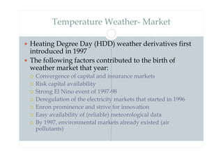
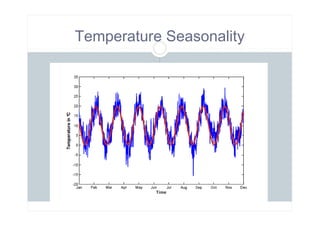
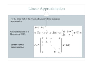
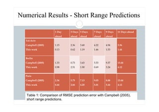
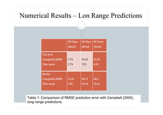
The document discusses nonlinear weather forecasting techniques used for pricing weather derivatives, particularly focusing on temperature modeling and the impact of various market factors that led to the establishment of weather markets in 1997. It includes methodologies like GARCH models and embedology algorithms to predict temperature trends and seasonal volatility. Additionally, it compares prediction accuracy against previous studies, highlighting methodologies and numerical results for short and long-term weather forecasts.

1. GAL ZAHAVI, YARON ROSENSTEIN
TECHNION-ISRAEL INSTITUTE OF TECHNOLOGY
THE WILLIAM DAVIDSON FACULTY OF INDUSTRIAL ENGINEERING & MANAGEMENT
Nonlinear Weather Forecasting for Weather Derivatives
Pricing

2. Temperature Weather- Market
Heating Degree Day (HDD) weather derivatives first
introduced in 1997
The following factors contributed to the birth of
weather market that year:
Convergence of capital and insurance markets
Risk capital availability
Strong El Nino event of 1997-98
Deregulation of the electricity markets that started in 1996
Enron prominence and strive for innovation
Easy availability of (reliable) meteorological data
By 1997, environmental markets already existed (air
pollutants)

3. Hedging Weather Risk CME

4. CME – Weather Products

5. Most common financial options
are:
• Futures (swaps)
• Calls
• Puts
( )
V N P X
= −
{ }
max ( ),0
V N P X
= −
{ }
max ( ),0
V N X P
= −
where
V is payoff
N is notional amount
P is the actual value of settlement index
X is the strike
X P
V
X P
X P

6. Cooling and Heating Degree
Days (CDD/HDD)
• Daily cooling (cdd) and
heating (hdd) degree
days:
{ }
{ }
,min ,max
ˆ
max 65 ,0
ˆ
max 65 ,0
ˆ
where is defined as
ˆ
2
o
i i
o
i i
i
i i
i
cdd t
hdd t
t
t t
t
≡ −
≡ −
+
≡
( )
1
( )
1
n M
M i
i
n M
M i
i
CDD cdd
HDD hdd
=
=
≡
≡
∑
∑
• Monthly cooling (CDD)
and heating (HDD)
degree days:
N(M) is the number of days
in month M

7. Temperature Time Series
0 500 1000
−10
−5
0
5
10
15
20
25
30
t (days)
T
(deg
C)
Paris
0 500 1000
−20
−15
−10
−5
0
5
10
15
20
25
30
t (days)
T
(deg
C)
Berlin
0 500 1000
5
10
15
20
25
30
t (days)
T
(deg
C)
Tel−Aviv

8. Temperature Seasonality

9. Temperature Modeling and Forecasting: Alaton et al. (2002)
Based on these two characteristics (positive tend and seaonality), Alaton, Djehiche and
Stillberger (2002) propose the following model to describe the average temperature at time t:
The model for temperature can be described as follows:
The parameters are estimated using the LS regression.
angle
phase
,
365
/
2
)
2
(
cos
sin
)
1
(
)
sin(
2
1
=
=
+
+
+
=
⇒
+
+
+
=
ϕ
π
ω
β
β
ϕ
wt
wt
t
Y
X
T
t
w
Z
t
Y
X
T
a
t
a
t
)
,
0
(
~
)
3
(
cos
sin
2
3
2
1
0
σ
η
η
γ
γ
γ
γ
IID
wt
wt
t
T
t
t
t +
+
+
+
=
i
i
i
i
i y
m
S
T σ
+
+
=
Seasonality Trend ARFIMA-FIGARCH
Seasonal volatility

10. Temperature Modeling and Forecasting:
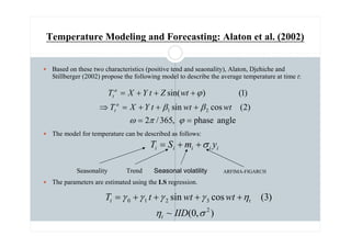
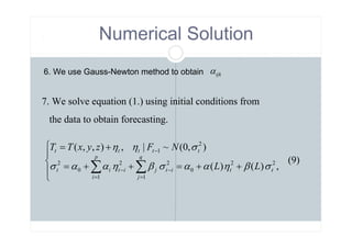
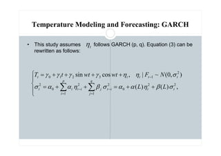
Alaton et al. (2002)
Alaton et al. (2002) obtain the following stochastic
differential equation in continuous form:
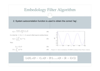
The above equation can be rewritten in discrete form:
can be estimated based on Equations (2) and (3).
can be obtained using the OLS regression and
)
5
(
)]
(
)
/
[( t
t
t
a
t
a
t
t dW
dt
T
T
dt
dT
dT σ
α +
−
+
=
a
j
T
( ) )
8
(
)
ˆ
1
(
ˆ
~
2
1
ˆ
1
2
1
1
2
∑
=
−
− −
−
−
−
=
µ
α
α
σ
µ
µ
N
j
j
a
j
j T
T
T
N
)
month
in
days
(
,
,
1
),
1
,
0
(
~
(7)
)
1
(
)
(
~
1
1
1
1
µ
η
η
σ
α
α
µ
µ
µ
N
N
j
N
T
T
T
T
T
T
j
j
j
a
j
a
j
a
j
j
j
K
=
+
−
+
=
−
−
≡ −
−
−
−
α̂
Time Trend
Mean-Reverting

11. Temperature and Forecasting Models: GARCH
This study assumes follows GARCH (p, q).
Equation (3) can be rewritten as follows:
)
9
(
,
)
(
)
(
)
,
0
(
~
|
,
cos
sin
2
2
0
1
2
1
2
0
2
2
1
3
2
1
0





+
+
=
+
+
=
+
+
+
+
=
∑
∑ =
−
=
−
−
t
t
q
j
i
t
j
p
i
i
t
i
t
t
t
t
t
t
L
L
N
F
wt
wt
t
T
σ
β
η
α
α
σ
β
η
α
α
σ
σ
η
η
γ
γ
γ
γ
t
η

12. Embedology Filter Algorithm
1. Time series is non-linearly filtered using Sauer (1991) non-linear filter. In this
method noise is projected onto a high dimensional manifold. Singular value
decomposition is used to obtain principal directions of the attractor, thus
obtaining clean signal.

13. 2. System autocorrelation function is used to obtain the correct ‘lag’.
Embedology Filter Algorithm

14. 3. False nearest neighbor analysis is performed to obtain the correct
dimension of the manifold.
Embedology Filter Algorithm

15. Embedology Algorithm
4. System is then ‘delayed’ (projected) to m dimensional space.

16. Non-Linear Dynamical System
5. Using the projected m dimensional system we fit a nonlinear system
of first order ODEs, based on Lorenz system.
( ) { }
m
i
t
x
f
dt
dx
j
i
i
,..,
1
,
, ∈
=
( ) l
k
kl
k
k
j
i x
x
b
x
a
t
x
f +
=
,
Where:
ijk
α Is the tensor of parameters, to be determined by the fitting.

17. 6. We use Gauss-Newton method to obtain ijk
α
. Numerical Solution
7. We solve equation (1.) using initial conditions from
the data to obtain forecasting.
)
9
(
,
)
(
)
(
)
,
0
(
~
|
,
)
,
,
(
2
2
0
1
2
1
2
0
2
2
1





+
+
=
+
+
=
+
=
∑
∑ =
−
=
−
−
t
t
q
j
i
t
j
p
i
i
t
i
t
t
t
t
t
t
L
L
N
F
z
y
x
T
T
σ
β
η
α
α
σ
β
η
α
α
σ
σ
η
η

18. Lorentz Equation’s – Physical Motivation
Deterministic nonperiodic flow
EN Lorenz - Journal of the atmospheric sciences, 1963 - journals.ametsoc.org
Cited by 10180 - Related articles - All 22 versions
“Forced Dissipative Systems”
i
k
j
ijk
k
j
j
ij
j
i
l
k
j
k
j
k
j
i
k
j
j
j
i
j
i
m
i
i
c
X
X
b
X
a
dt
dX
X
X
X
L
X
X
X
X
f
X
X
f
dt
dX
t
X
X
X
f
X
+
+
=
∆
∆
∆
+
∆
∆
∂
∂
∂
+
∆
∂
∂
=
⇒
=
∑
∑
∑
∑
,
2
,
2
1
)
,
,
(
)
,
,.....,
,
(

19. Saltzman - Equation
Finite amplitude free convection as an initial value
J. atmos. Sci, 1962

20. Dynamical System of ODE
Base assumption on the solution form
Resulting ODE

21. Real time Examples
Lorenz attractor from time series

22. Temperature Modeling and Forecasting: GARCH
• This study assumes follows GARCH (p, q). Equation (3) can be
rewritten as follows:





+
+
=
+
+
=
+
+
+
+
=
∑
∑ =
−
=
−
−
,
)
(
)
(
)
,
0
(
~
|
,
cos
sin
2
2
0
1
2
1
2
0
2
2
1
3
2
1
0
t
t
q
j
i
t
j
p
i
i
t
i
t
t
t
t
t
t
L
L
N
F
wt
wt
t
T
σ
β
η
α
α
σ
β
η
α
α
σ
σ
η
η
γ
γ
γ
γ
t
η

23. ))
0
(
)
(
(
))
0
(
)
(
(
))
0
(
)
(
(
)
(
,
)
0
(
)
0
(
)
0
(
)
cos(
0
0
0
)
sin(
0
0
0
)
(
)
(
)
(
,
0
0
0
0
0
0
3
3
2
2
2
1
3
2
1
3
2
1
4
3
3
2
1
3
2
1
4
3
3
2
1
X
t
X
X
t
X
X
t
X
t
T
c
c
c
X
X
X
wt
wt
ct
t
X
t
X
t
X
X
X
X
c
X
X
X
dt
d
−
+
−
+
+
=










+




















=






























−
=










γ
γ
γ
γ
Alaton 2002 – Linear ODE solution
We present the particular case of Alaton 2002 in the framework of Lorentz 1963.

24. Linear Approximation
5. For the linear part of the dynamical system














=




























=














⇒
=
m
m
mm
m
m
m X
X
X
X
X
X
X
a
a
a
a
a
a
a
X
X
X
dt
d
X
A
X
dt
d
)
0
(
)
0
(
)
0
(
, 2
1
0
2
1
1
22
21
1
12
11
2
1
M
jk
α Is the tensor of
parameters, to be
determined by the fitting.
General Solution For N
Dimensional ODE.
)
0
(
0
0
0
0
0
0
)
(
)
0
(
)
(
1
1
1
2
1
X
S
e
e
e
S
t
X
X
S
e
S
t
X
S
D
S
A
t
t
t
Dt
m
−
−
−
⋅
















⋅
=
⋅
⋅
=
⇒
⋅
⋅
=
λ
λ
λ
O
O
M
L
For D the Eigenvalue
representation of A
If Eigenvalue are
purely imaginary
we get a Furrier
decomposition

25. Linear Approximation
For the linear part of the dynamical system without a diagonal
representation
General Solution For m
Dimensional ODE.
)
0
(
0
0
1
1
0
0
1
)
0
(
!
)
(
)
0
(
)
(
1
2
1
1
0
1
1
X
S
S
J
X
S
n
Jt
S
X
S
e
S
t
X
S
J
S
A
m
n
n
Jt
−
−
∞
=
−
−
⋅
















⋅
=
⋅








⋅
=
⋅
⋅
=
⇒
⋅
⋅
=
∑
λ
λ
λ
O
O
M
L
Jordan Normal
decomposition
1
λ

26. 1 Day
ahead
3 Days
ahead
5 Days
ahead
7 Days
ahead
9 Days
ahead
11 Days ahead
Tel-Aviv
Campbell (2005)
This work
1.15
0.13
2.36
0.62
3.40
1.19
4.22
1.46
4.94
1.53
5.56
1.44
Berlin
Campbell (2005)
This work
1.33
0.98
0.73
2.51
3.43
1.90
5.53
0.69
9.37
3.24
13.44
4.12
Paris
Campbell (2005)
This work
2.34
0.44
5.75
2.66
7.13
4.20
9.03
5.01
8.88
5.44
13.44
4.12
Numerical Results - Short Range Predictions
Table 1: Comparison of RMSE prediction error with Campbell (2005),
short range predictions.

27. 30 Days
ahead
60 Days
ahead
90 Days
ahead
Tel-Aviv
Campbell (2005)
This work
9.74
2.74
36.65
3.51
61.25
8.51
Berlin
Campbell (2005)
This work
11.81
1.87
48.71
19.14
68.3
15.41
Numerical Results – Lon Range Predictions
Table 1: Comparison of RMSE prediction error with Campbell (2005),
long range predictions.

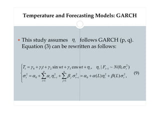
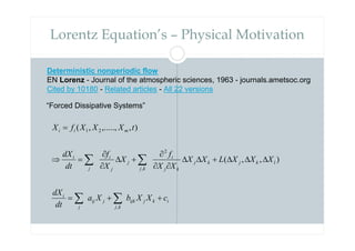
28. HDD/CDD Option Price Formula . Alaton et al. 2002)
)
15
(
2
)
(
)
(
)
(
)
(
]
|
}
0
,
[max{
(14)
2
)
(
)
(
)
(
)
(
]
|
}
0
,
[max{
2
2
2
2
1
2
)
(
0
)
(
)
(
2
)
(
)
(
)
(




















−
+
















−
Φ
−
Φ
−
=
−
=
−
=








+
−
Φ
−
=
−
=
−
=








−
−
−
−
−
−
−
−
−
−
−
−
∞
−
−
−
−
∫
∫
n
n
n
n
n
n
n
n
n
n
n
n
e
e
K
e
dx
x
f
x
K
e
F
H
K
E
e
p
e
K
e
dx
x
f
K
x
e
F
K
H
E
e
c
n
n
n
n
n
t
t
r
K
H
t
t
r
t
n
Q
t
t
r
t
n
n
n
t
t
r
K
H
t
t
r
t
n
Q
t
t
r
t
σ
µ
α
α
π
σ
σ
µ
α
µ
π
σ
α
µ

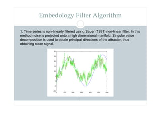
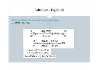
29. Alaton et al. (2002) estimate the conditional variance
.
0
)
20
(
]
)[
1
)(
2
/
1
(
]
|
,
[
)
19
(
]
)[
1
)(
2
/
1
(
]
|
[
)
18
(
]
)[
1
)(
/
(
)
(
]
|
[
2
2
2
2
1
2
)
(
2
2
2
2
1
2
2
1
)
(
u
t
s
e
e
F
T
T
Cov
e
F
T
Var
e
T
e
T
T
F
T
E
t
s
s
s
t
s
u
t
t
s
s
s
t
t
s
s
m
t
s
t
m
s
s
s
t
Q
≤
≤
≤
+
+
+
−
=
+
+
+
−
=
+
+
+
−
−
+
−
=
+
+
−
−
−
+
+
−
+
+
−
−
−
σ
σ
σ
α
σ
σ
σ
α
σ
σ
σ
α
λ
α
α
α
α
α
L
L
L

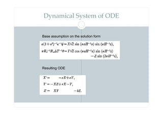
30. First-Order and Second-Order Moments of Hn and Cn
( )
( )
)
27
(
]
│
,
[
2
]
|
[
]
│
[
)
26
(
23
]
|
[
|
23
]
|
[
)
25
(
]
|
,
[
2
]
|
[
]
|
[
)
24
(
]
|
[
23
|
23
]
|
[
1
1
1
1
1
1
∑∑
∑
∑
∑
∑∑
∑
∑
∑
=
=
=
=
=
=
+
≈
−
=
−
≈
+
≈
−
=
−
≈
j
i
t
t
t
n
t t
t
t
n
n
i t
t
Q
t
n
i t
Q
t
n
Q
j
i
t
t
t
n
t t
t
t
n
n
i t
t
Q
t
n
i t
Q
t
n
Q
F
T
T
Cov
F
T
Var
F
C
Var
n
F
T
E
F
n
T
E
F
C
E
F
T
T
Cov
F
T
Var
F
H
Var
F
T
E
n
F
T
n
E
F
H
E
j
i
i
i
j
i
i
i

31. Thank You ☺