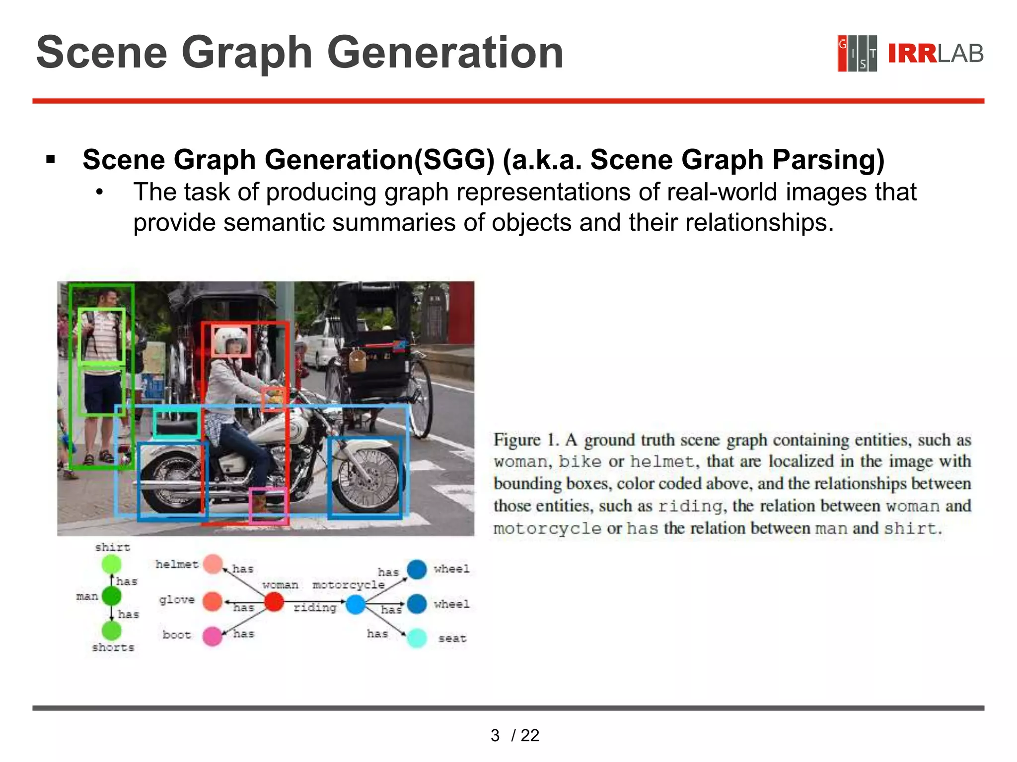
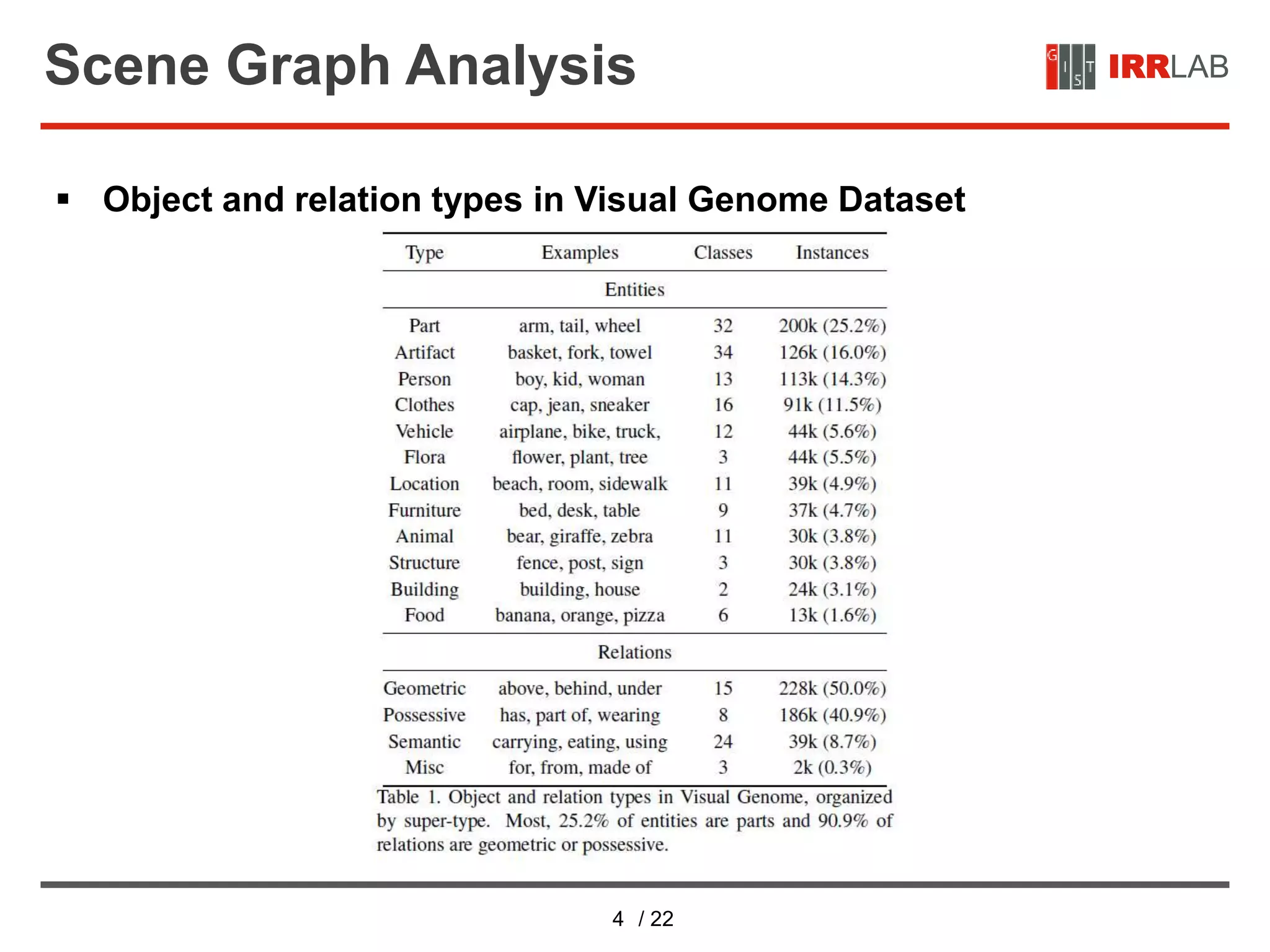
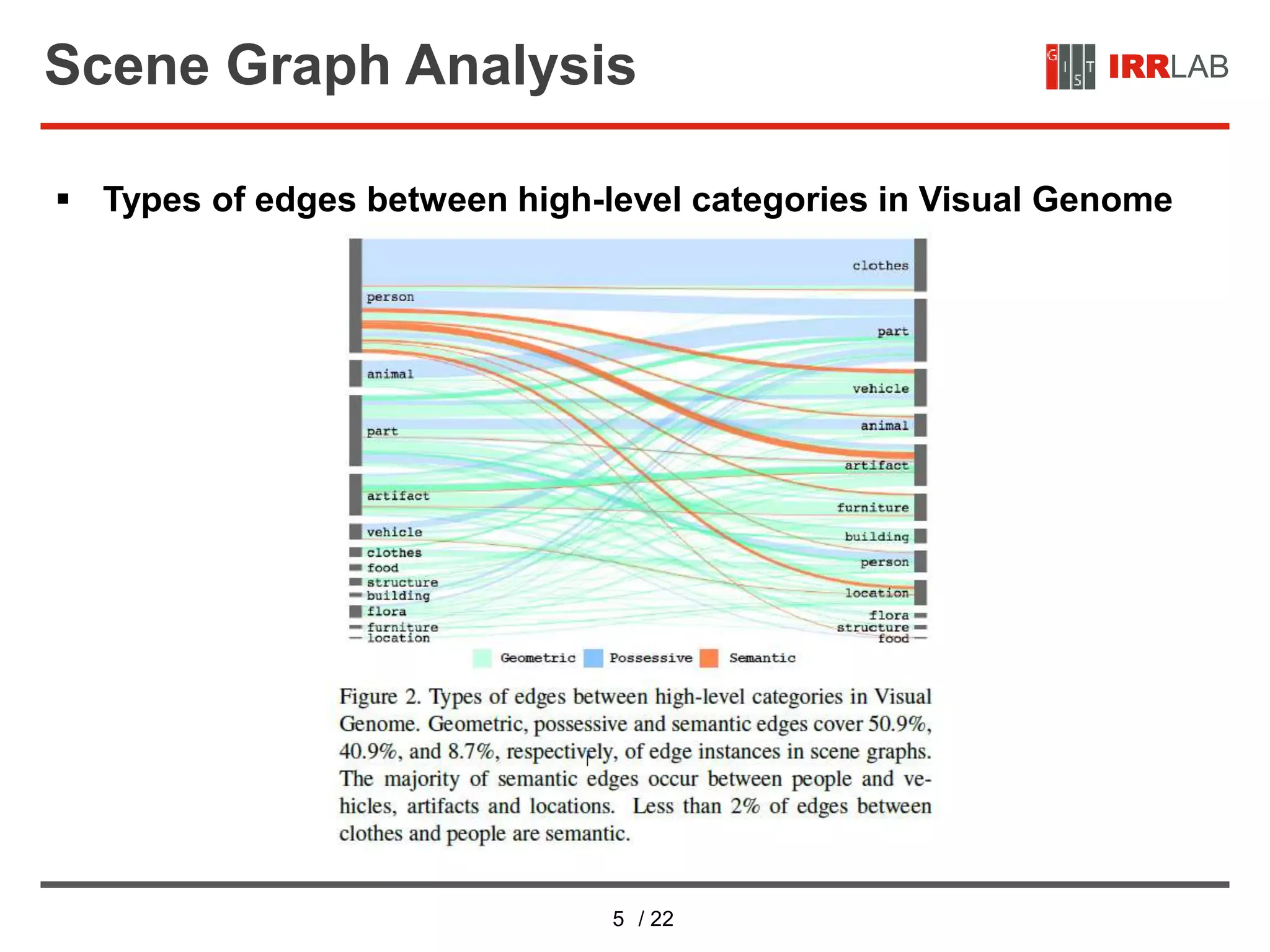
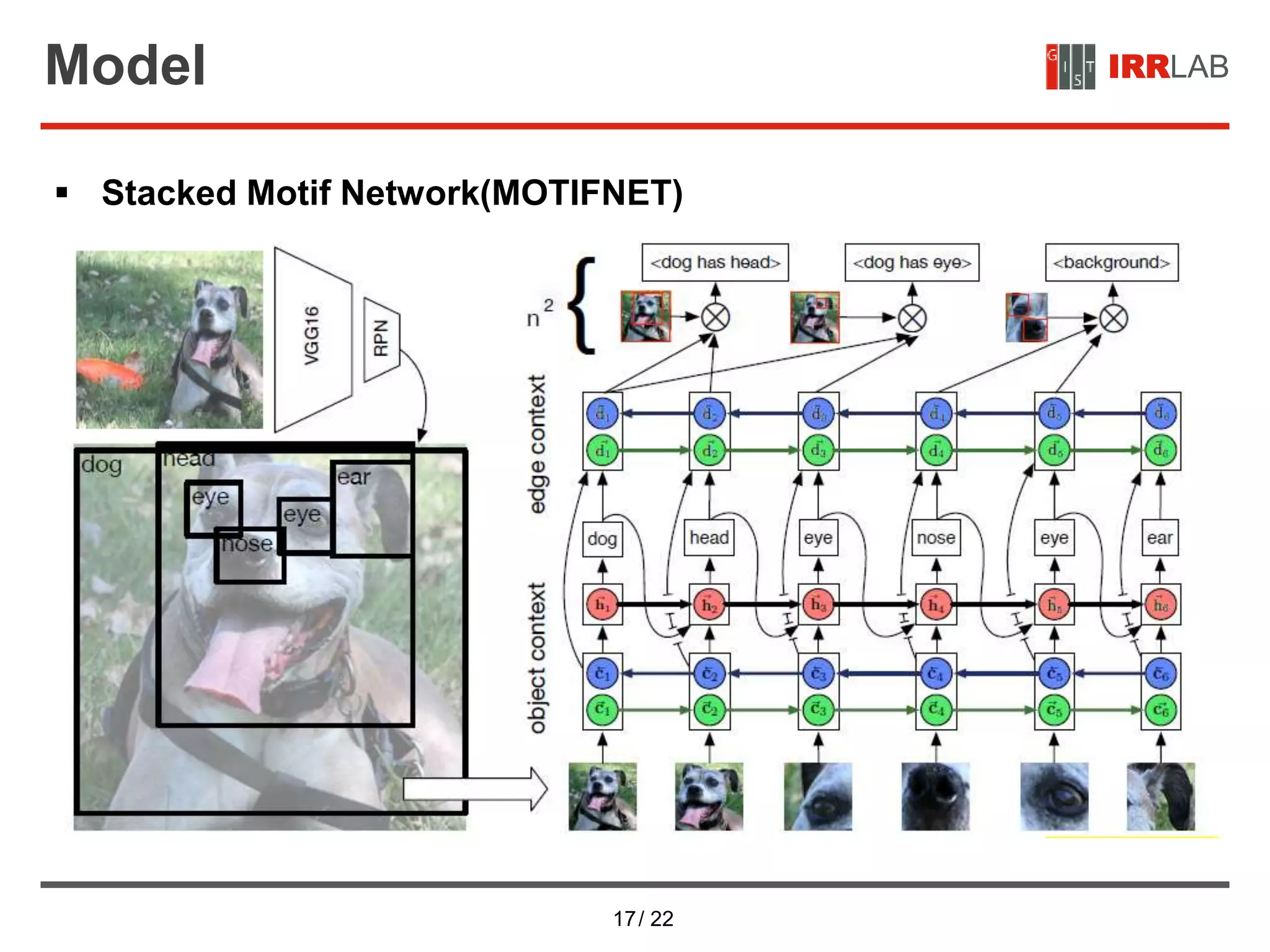
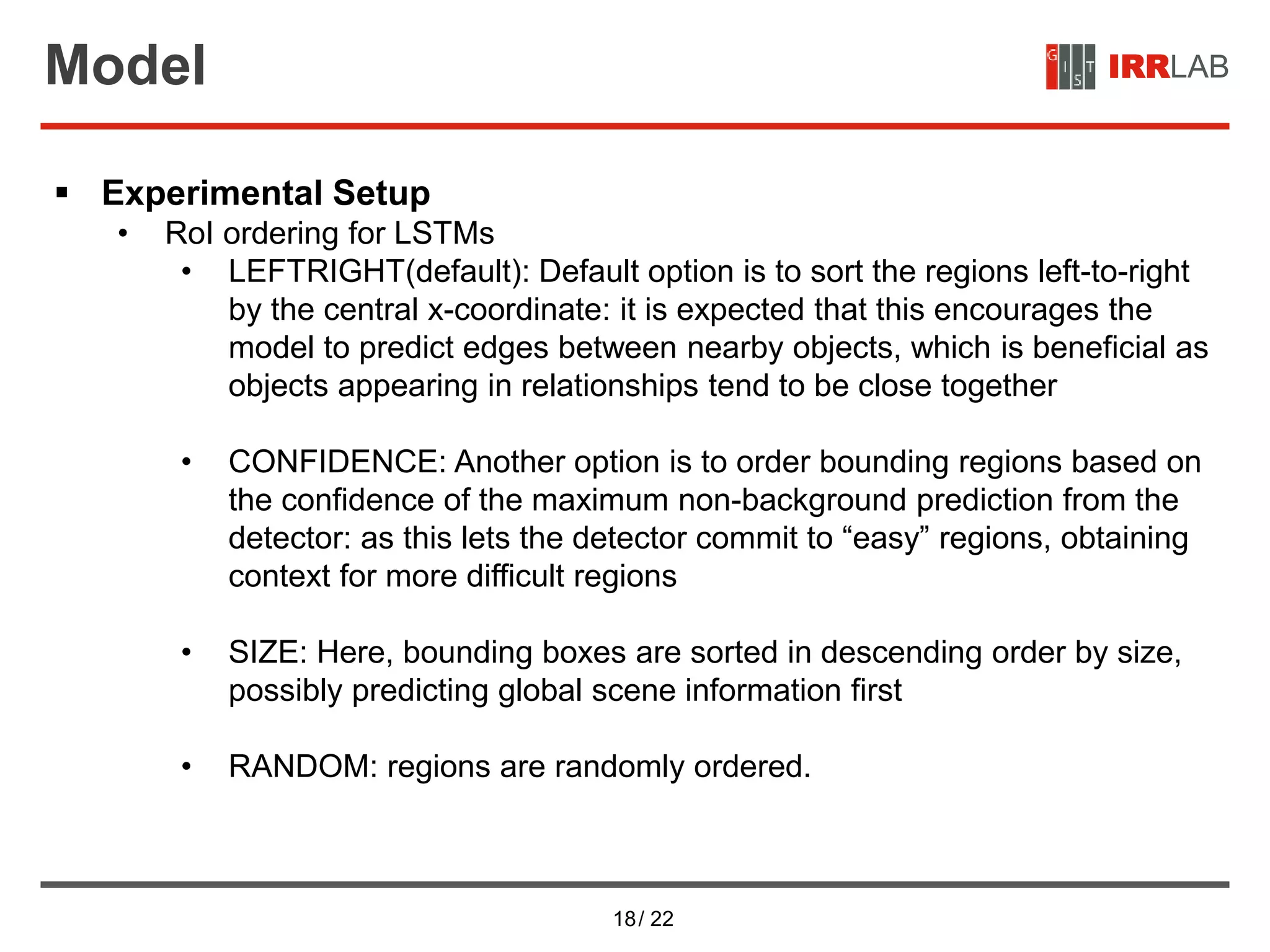
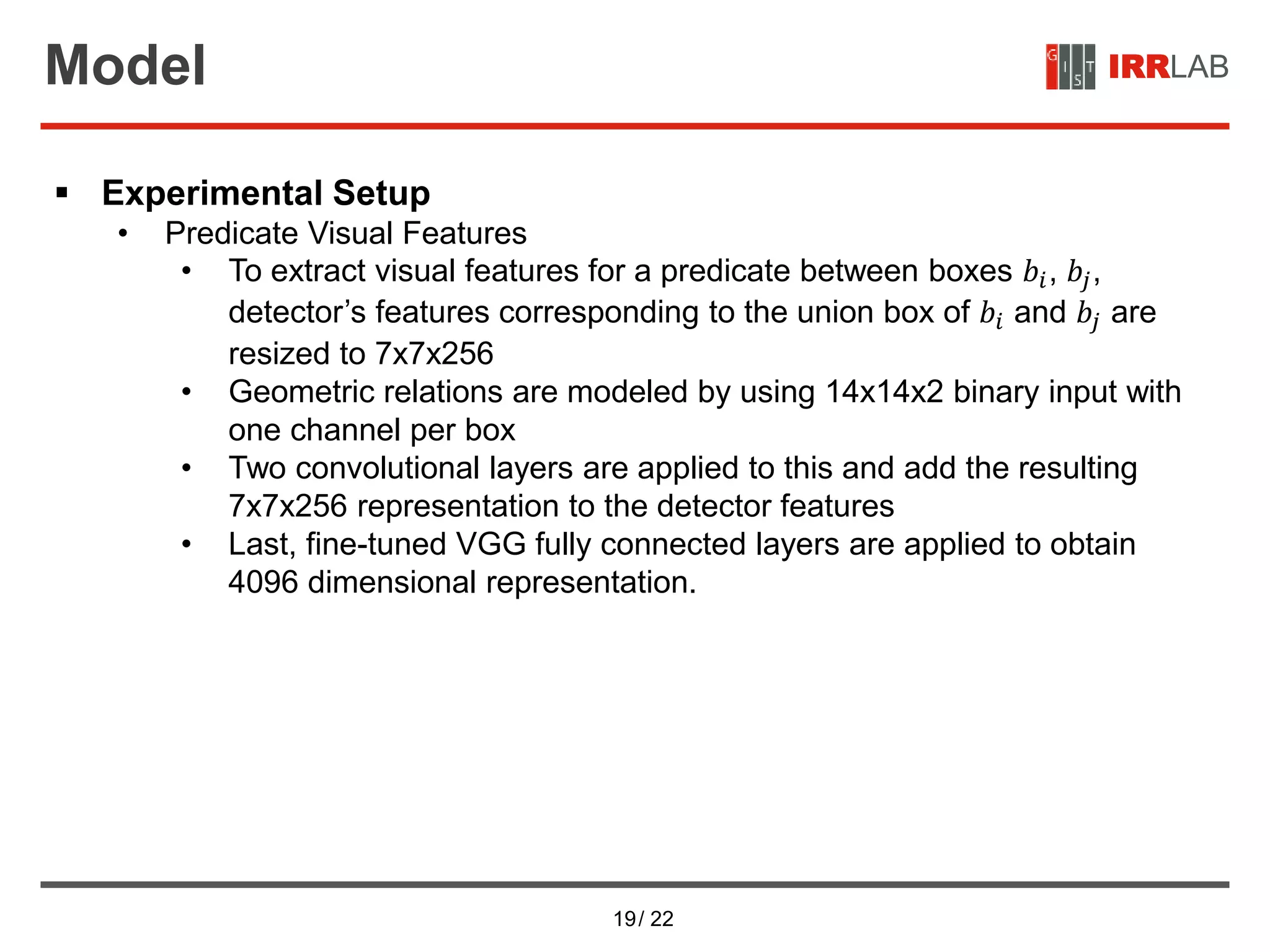
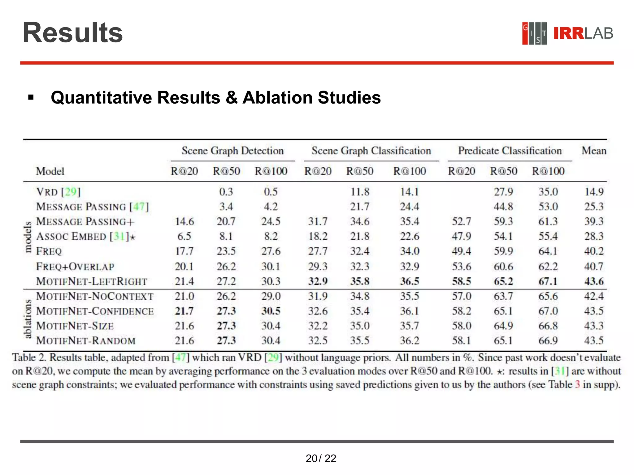
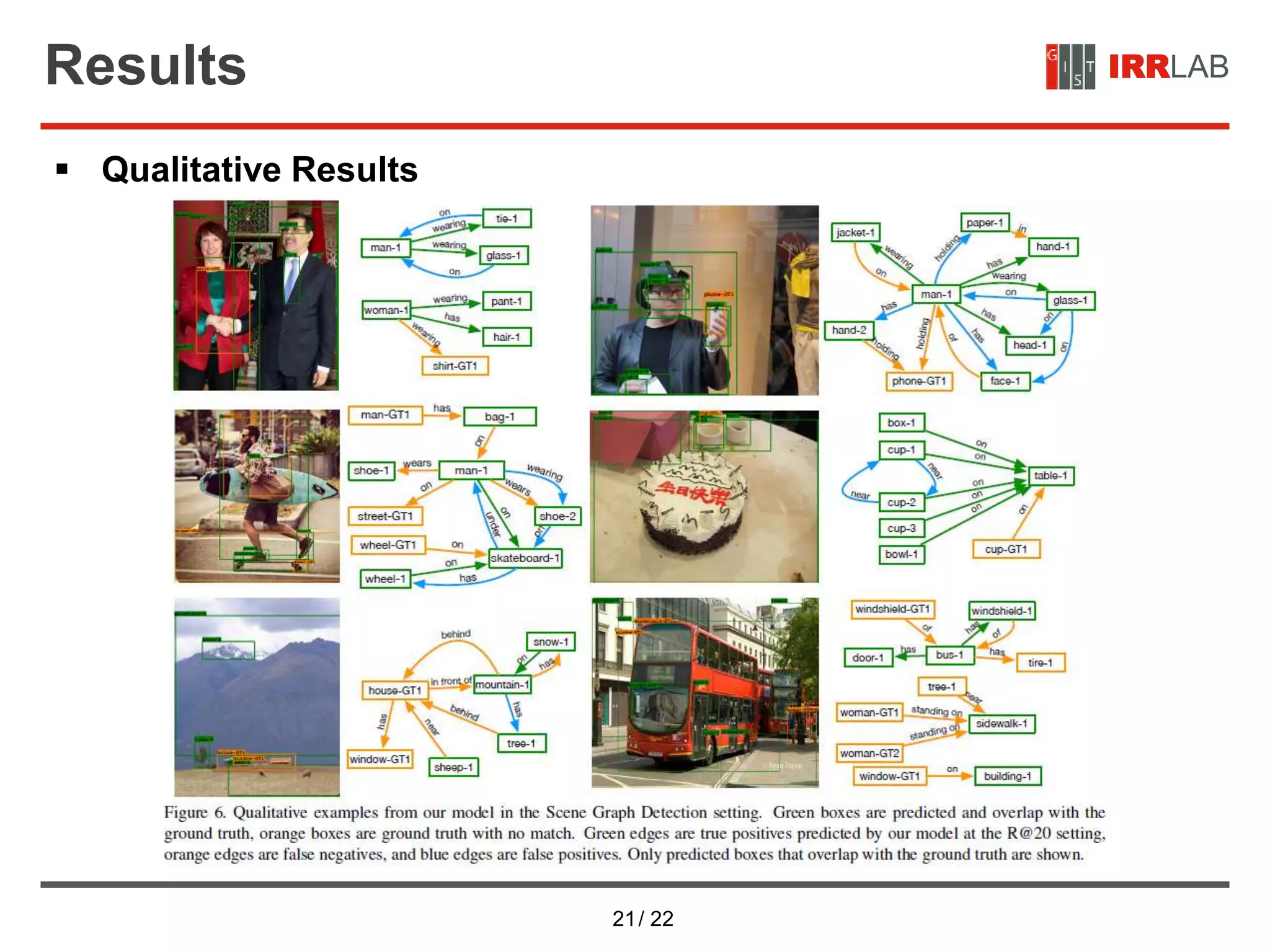
The document presents a detailed overview of a neural network approach for scene graph parsing using global context, called Neural Motifs. It discusses scene graph generation, analysis of object and relationship types, the architecture of the stacked motif network, and experimental results, emphasizing the significance of contextualized object and relation representations. The methods include advanced object detection techniques, the use of LSTMs for context encoding, and evaluations of the model's performance through quantitative and qualitative results.

![11 / 22
IRRLABModel
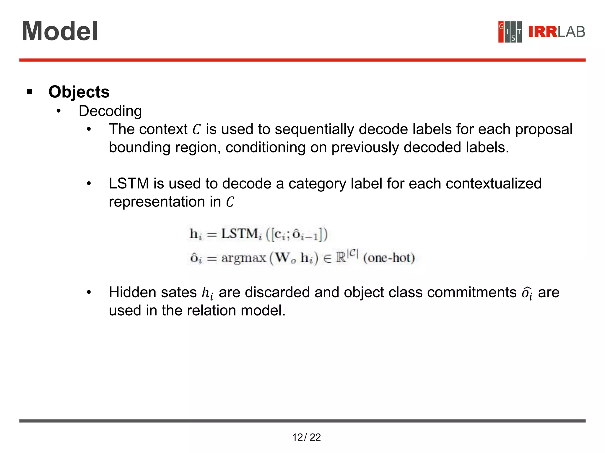
Objects
• Context Encoding
• Construct a contextualized representation of object prediction based
on the set of proposal regions 𝐵
• Element of 𝐵 are first organized into a linear sequence,
[(𝑏1, 𝑓1, 𝑙1), … , (𝑏 𝑛, 𝑓𝑛, 𝑙 𝑛)].
• The object context, 𝐶, is then computed using a bidirectional LSTM
• 𝐶 = [𝑐1, … , 𝑐 𝑛] contains the final LSTM layer’s hidden states for each
element in the linearization of 𝐵
• 𝑊1 is a parameter matrix that maps the distribution of predicted classes, 𝑙1
to ℝ100
.
• The biLSTM allows all elements of 𝐵 to contribute information about
potential object identities.](https://image.slidesharecdn.com/neuralmotifsscenegraphparsingwithglobalcontext-200710120140/75/Neural-motifs-scene-graph-parsing-with-global-context-11-2048.jpg)
![13/ 22
IRRLABModel
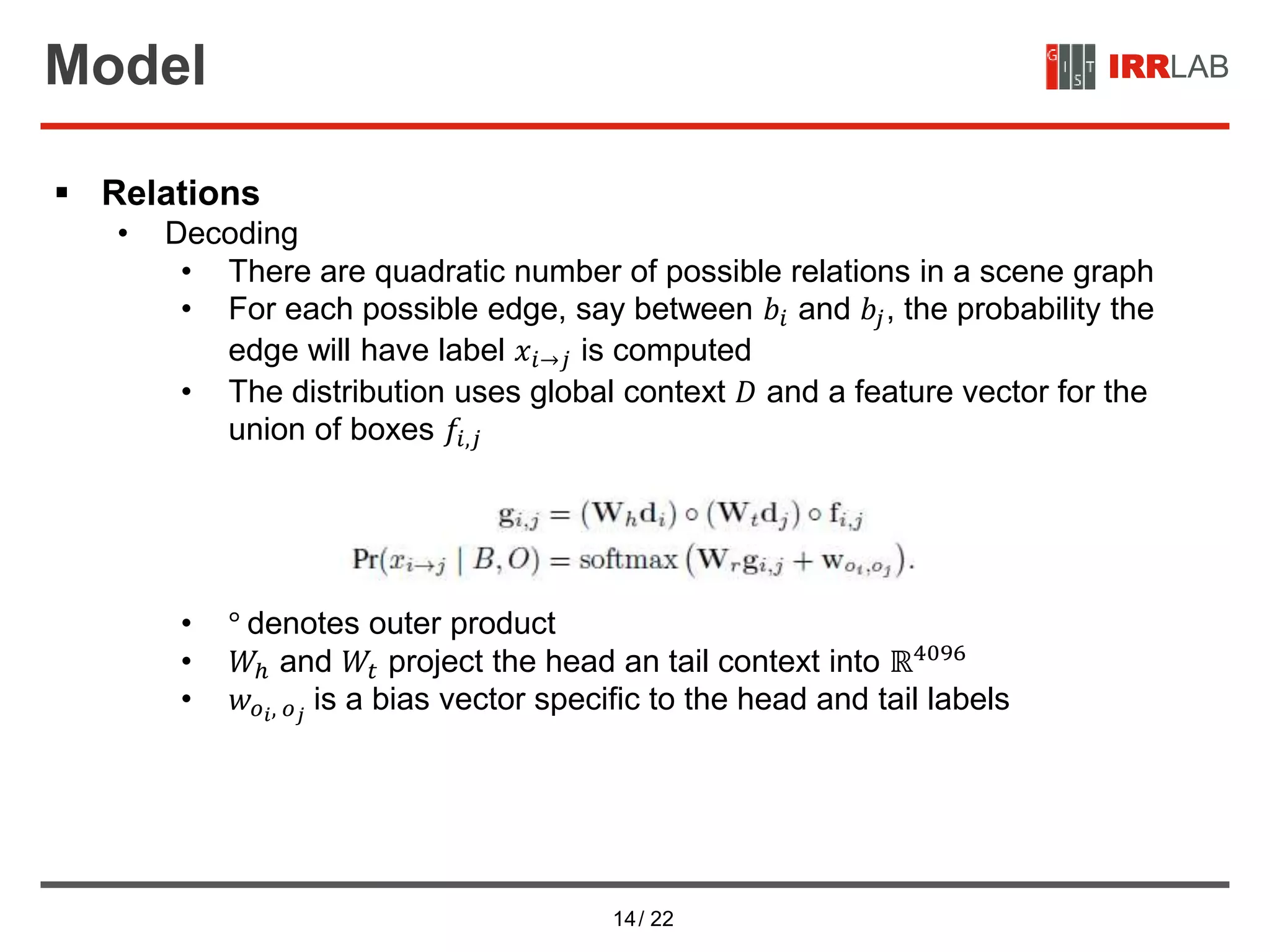
Relations
• Context Encoding
• Construct a contextualized representation of bounding regions 𝐵 and
objects 𝑂 using additional bi-directional LSTM layers
• Where the edge context 𝐷 = [𝑑1, … , 𝑑 𝑛] contains the states for each
bounding region at the final layer, and 𝑊2 is a parameter matrix
mapping 𝑜𝑖 into ℝ100](https://image.slidesharecdn.com/neuralmotifsscenegraphparsingwithglobalcontext-200710120140/75/Neural-motifs-scene-graph-parsing-with-global-context-13-2048.jpg)


![[NS][Lab_Seminar_241118]Relation Matters: Foreground-aware Graph-based Relati...](https://cdn.slidesharecdn.com/ss_thumbnails/nslabseminar241118fgrr-241118111529-1ff1aba4-thumbnail.jpg?width=640&height=640&fit=bounds)


![[NS][Lab_Seminar_250407]AlignmentLearning.pptx](https://cdn.slidesharecdn.com/ss_thumbnails/nslabseminar250407alignmentlearning-250407124309-1acb59f1-thumbnail.jpg?width=640&height=640&fit=bounds)
![[NS][Lab_Seminar_250106]SAM-Aware Graph Prompt Reasoning Network for Cross-Do...](https://cdn.slidesharecdn.com/ss_thumbnails/nslabseminar250106gprn-250106075150-b64c5cde-thumbnail.jpg?width=640&height=640&fit=bounds)