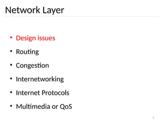
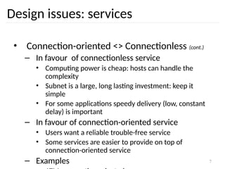
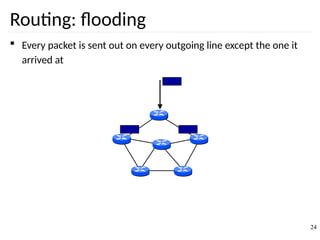
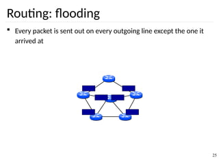
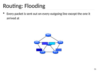
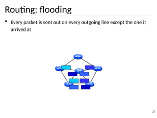
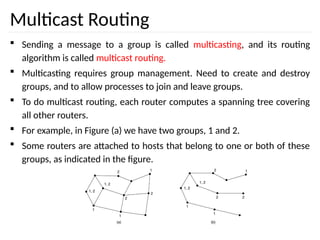
The document discusses the design issues and protocols of the network layer, focusing on topics like routing, congestion control, internetworking, and quality of service. It details various routing algorithms, including the differences between distance vector and link state routing, and their respective mechanisms for ensuring data delivery. Additionally, it covers types of network services, such as connection-oriented and connectionless services, as well as broadcast, multicast, and anycast transmission methods.

![9
7
4
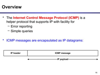
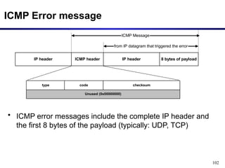
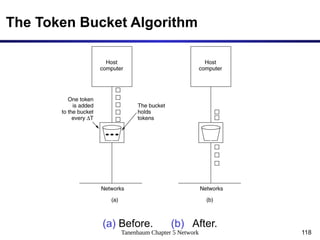
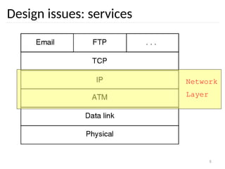
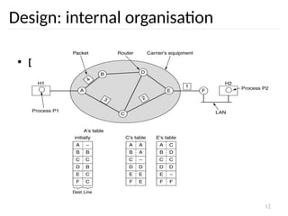
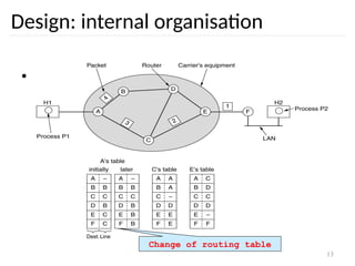
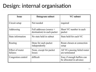
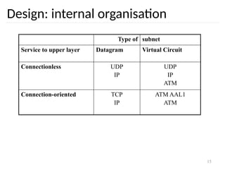
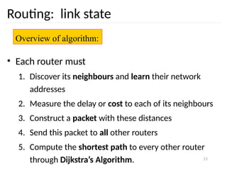
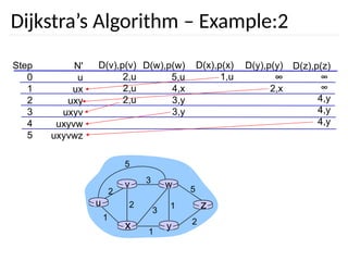
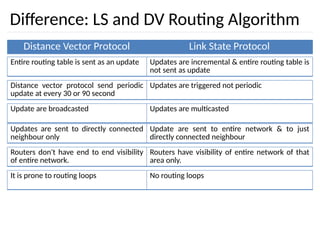
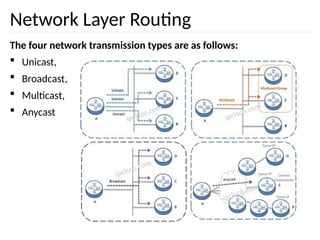
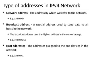
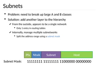
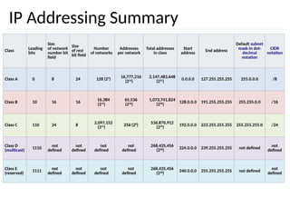
Design: internal organisation
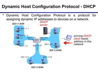
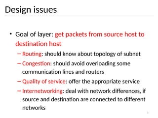
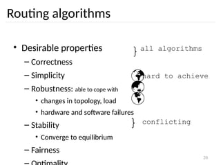
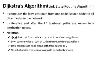
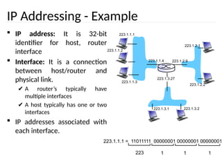
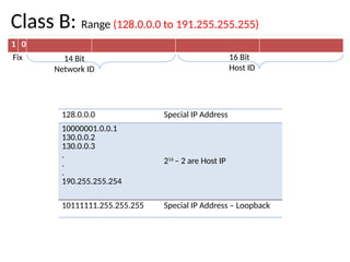
• Virtual circuits
– Routes chosen at connection time
– Connection identified by a virtual circuit number
(VCn)
– Primary service of subnet is connection-oriented
Physical
Data Link
Network
Transport
Physical
Data Link
Network
Transport
Routing problem: map
[Incoming line, VCn]
[outgoing line, VCn]](https://image.slidesharecdn.com/networklayer-241109171833-db724b11/85/Network-layer-pptx-9-320.jpg)
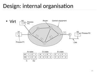
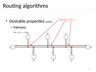

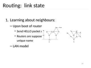
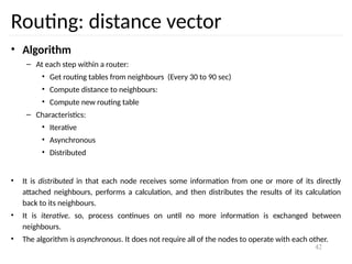


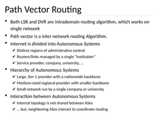

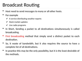
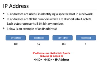
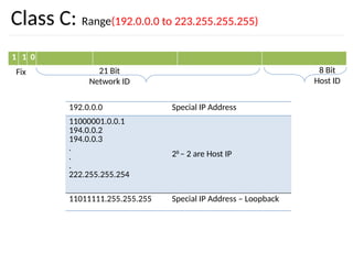
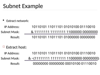
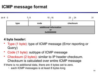
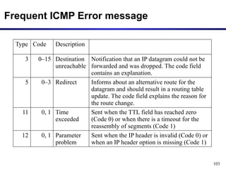
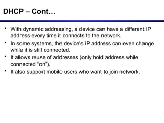
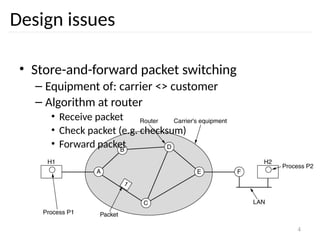
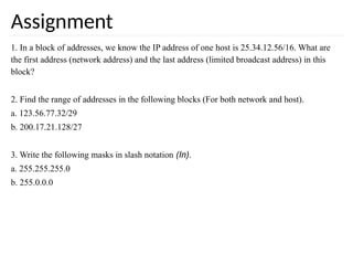
![How many subnets from given subnet mask?
To calculate the number of subnets provided by given subnet
mask we use 2N
, where N = number of bits borrowed from host
bits to create subnets.
For example in 192.168.1.0/27, N is 3.
By looking at address we can determined that this address is
belong to class C and default subnet mask 255.255.255.0 [/24 in
CIDR].
In given address we borrowed 27 - 24 = 3 host bits to create
subnets.
Now 23
= 8, so our answer is 8 (number of subnets ).](https://image.slidesharecdn.com/networklayer-241109171833-db724b11/85/Network-layer-pptx-88-320.jpg)
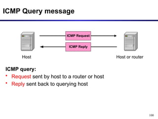
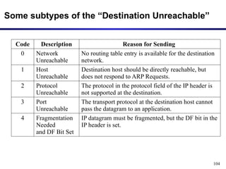
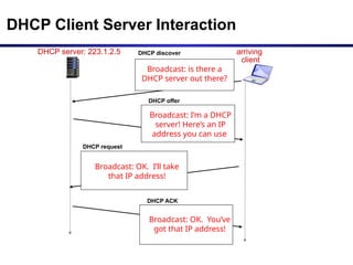
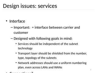
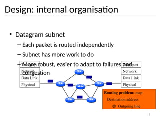
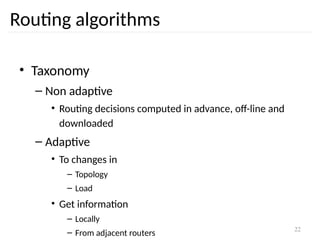
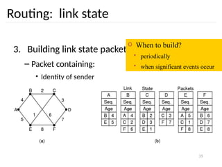
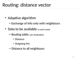
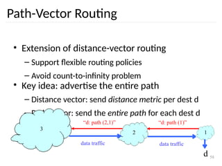
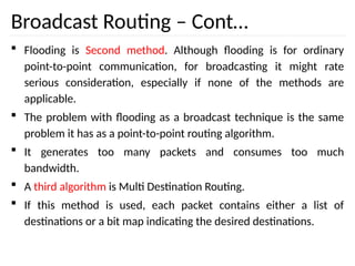
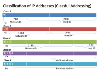
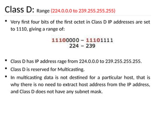
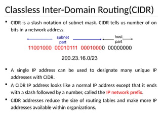
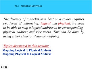
![What are the total hosts?
Total hosts are the hosts available per subnet
To calculate total hosts use formula 2H
= Total hosts
H is the number of host bits
For example in address 192.168.1.0/26
We have 32 - 26
1. [Total bits in IP address - Bits consumed by network address] = 6
2. Total hosts per subnet would be 26
= 64](https://image.slidesharecdn.com/networklayer-241109171833-db724b11/85/Network-layer-pptx-89-320.jpg)
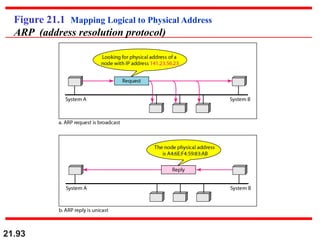
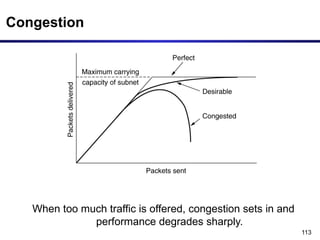
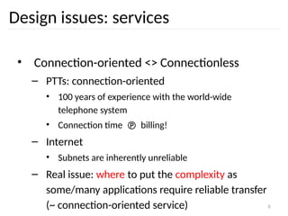
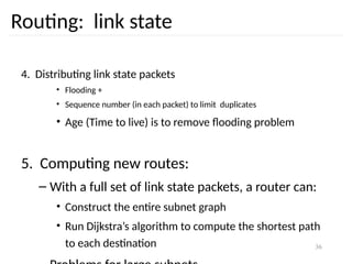
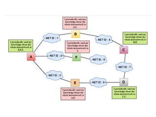
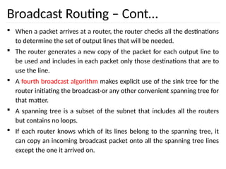
![97
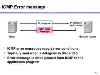
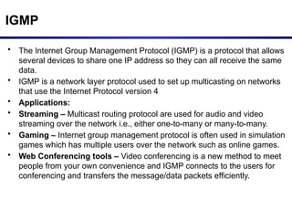
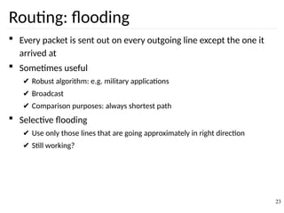
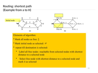
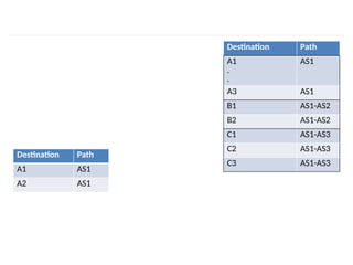
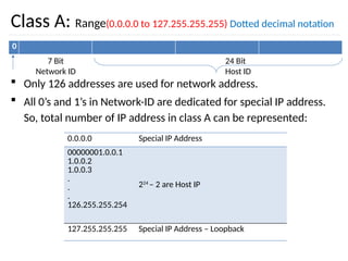
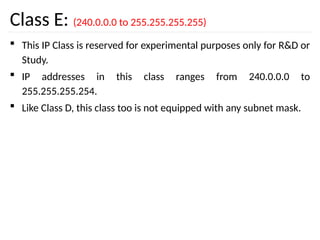
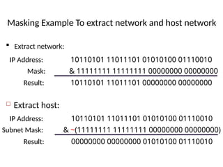
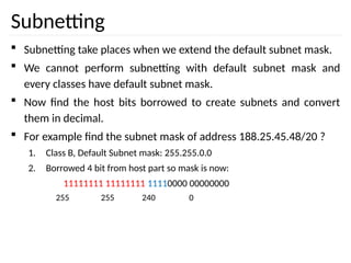
• The IP (Internet Protocol) relies on several other protocols to
perform necessary control and routing functions:
• Control functions (ICMP): [**ping and traceroute**]
• Multicast signaling (IGMP)
• Setting up routing tables (RIP, OSPF, BGP, PIM, …)
Control
Routing
ICMP IGMP
RIP OSPF BGP PIM
Internet Control Message Protocol (ICMP)](https://image.slidesharecdn.com/networklayer-241109171833-db724b11/85/Network-layer-pptx-97-320.jpg)