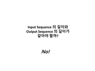
[Korean Version]
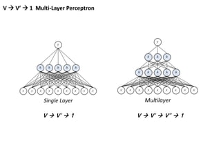
Multiple Vector Encoding techniques for Deep learning.
This article contains 1) RNN 2) Attention mechanism and 3) CNN for multiple vector encoding.
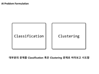
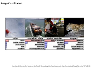
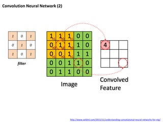
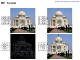
Image Classification
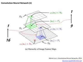
from AlexKrizhevsky, Ilya Sutskever, Geoffrey E. Hinton, ImageNet Classification with Deep Convolutional Neural Networks, NIPS, 2012.
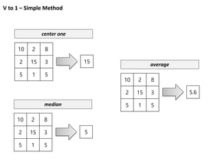
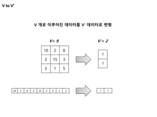
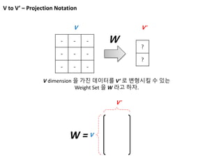
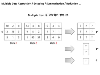
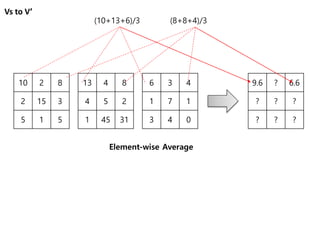
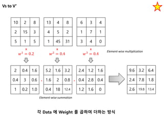
Vs to V’
102 8
2 15 3
5 1 5
13 4 8
4 5 2
1 45 31
6 3 4
1 7 1
3 4 0
𝑤1
= 0.2 𝑤2
= 0.4 𝑤3
= 0.4
X X X
2 0.4 1.6
0.4 3 0.6
1 0.2 1.0
5.2 1.6 3.2
1.6 2 0.8
0.4 18 12.4
2.4 1.2 1.6
0.4 2.8 0.4
1.2 1.6 0
9.6 3.2 6.4
2.4 7.8 1.8
2.6 19.8 13.4
+ +
Element-wise multiplication
Element-wise summation
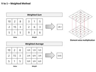
각 Data 에 Weight 를 곱하여 더하는 방식
30.
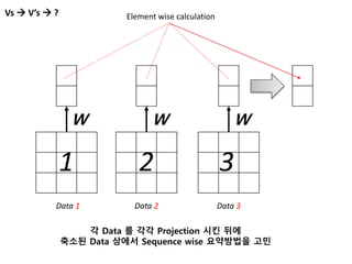
Vs V’s ?
Data 1 Data 2 Data 3
1 2 3
Element wise calculation
각 Data 를 각각 Projection 시킨 뒤에
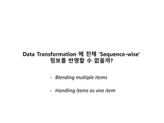
축소된 Data 상에서 Sequence wise 요약방법을 고민
W W W
31.
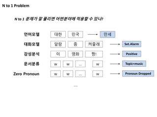
N to 1Problem
N to 1 문제가 잘 풀리면 어떤분야에 적용할 수 있나?
언어모델 대한 민국 만세
대화모델 알람 좀 Set.Alarm켜줄래
감성분석 이 영화 Positive짱!
문서분류 w w Topic=music… w
Zero Pronoun w w Pronoun Dropped… w
….
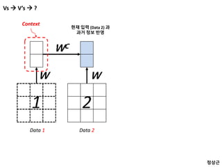
Vs V’s ?
Data 1 Data 2
1 2
W
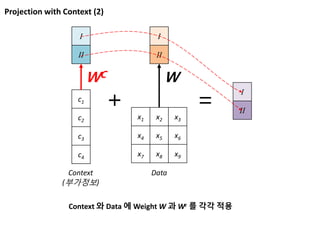
WC
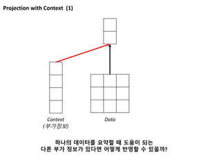
Context
현재 입력 (Data 2) 과
과거 정보 반영
W
정상근
35.
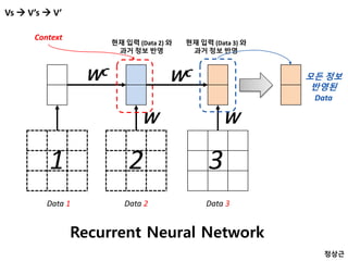
Vs V’s V’
Data 1 Data 2
1 2
W
WC
Context
현재 입력 (Data 2) 와
과거 정보 반영
Data 3
3
W
WC
현재 입력 (Data 3) 와
과거 정보 반영
모든 정보
반영된
Data
Recurrent Neural Network
정상근
36.
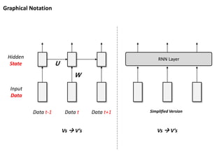
Graphical Notation
Data t-1Data t Data t+1
W
Input
Data
Hidden
State U
RNN Layer
Simplified Version
Vs V’s Vs V’s
37.
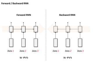
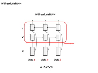
Forward / BackwardRNN
Data 1 Data 2 Data 3 Data 1 Data 2 Data 3
Forward RNN Backward RNN
Vs V’s Vs V’s
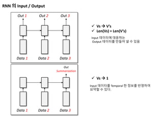
RNN 의 Input/ Output
Data 1 Data 2 Data 3
Out 1 Out 2 Out 3
Vs V’s
Len(Vs) = Len(V’s)
Input 데이터에 대응하는
Output 데이터를 만들어 낼 수 있음
Data 1 Data 2 Data 3
Out
Summarization
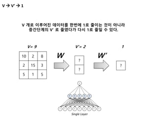
Vs 1
Input 데이터를 Temporal 한 정보를 반영하여
요약할 수 있다.
41.
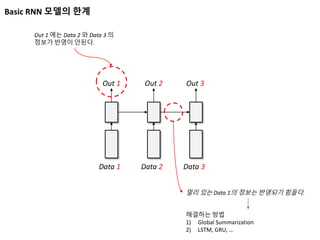
Basic RNN 모델의한계
Data 1 Data 2 Data 3
Out 1 Out 2 Out 3
Out 1 에는 Data 2 와 Data 3 의
정보가 반영이 안된다.
멀리 있는 Data 1의 정보는 반영되기 힘들다.
해결하는 방법
1) Global Summarization
2) LSTM, GRU, …
42.
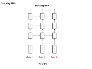
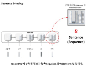
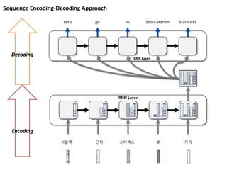
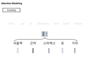
Sequence Encoding
가장 마지막RNN node 의
Hidden Variable
Sentence
(Sequence)
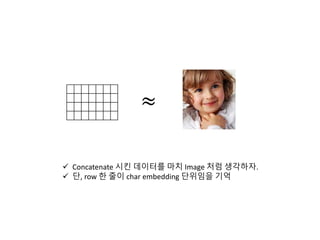
≈
Idea : RNN 에 누적된 정보가 결국 Sequence 의 Vector Form 일 것이다.
[참고] Translation Pyramid
BernardVauquois' pyramid showing comparative
depths of intermediary representation, interlingual
machine translation at the peak, followed by transfer-
based, then direct translation.
[ http://en.wikipedia.org/wiki/Machine_translation]
46.
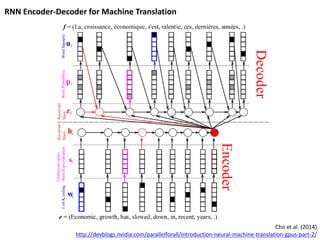
RNN Encoder-Decoder forMachine Translation
Cho et al. (2014)
http://devblogs.nvidia.com/parallelforall/introduction-neural-machine-translation-gpus-part-2/
47.
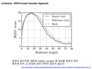
Limitation - RNNEncoder-Decoder Approach
문장이 길어지면, 제한된 hidden variable 에 정보를 충분히 담지
못하게 되어, 긴 문장의 경우 번역이 잘되지 않는다.
http://devblogs.nvidia.com/parallelforall/introduction-neural-machine-translation-gpus-part-3/
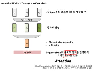
Attention Without Context– In/Out View
x1 x2 x3
Vs V
Global Summarization 개념은 RNN 과 상관없지만, Context 가 RNN 의 결과물과
연동되는 경우가 많기 때문에 advanced RNN 테크닉으로 보통 언급됨.
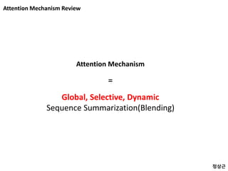
Sequence Data 에 중요도 정보를 반영하여
요약한 Data 를 만듦
Attention
x1 x2 x3
- 각 Data 중 더 중요한 데이터가 있을 것
중요도 반영
- 중요도 반영
Xs
- Element wise summation
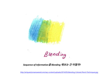
- = Blending
53.
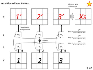
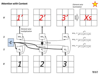
Attention without Context
a1a2 a3
1 2 3
A A A
V
1
wa1 wa2 wa31
1’ 2’ 3’V
𝑤𝑎1 =
𝑒 𝑎1
𝑒 𝑎1 + 𝑒 𝑎2 + 𝑒 𝑎3
𝑤𝑎2 =
𝑒 𝑎2
𝑒 𝑎1 + 𝑒 𝑎2 + 𝑒 𝑎3
𝑤𝑎3 =
𝑒 𝑎3
𝑒 𝑎1 + 𝑒 𝑎2 + 𝑒 𝑎3
Element wise
multiplication
Softmax
Xs
Element wise
Summation
정상근
Context 반영 방법
concat
어떻게C 와 xi 을
조합할까?
xi
C
X W
𝑠𝑐𝑜𝑟𝑒 = 𝑣 𝑇
tanh(𝑊 𝑥𝑖; 𝑐 )
concatenate
[ 1 x (V+K) ] [ (V+K) x M ]
K
V
X VT
[ M x 1 ]
[ 1 x M ]
general
xi
XWC X
[ 1 x K ] [ K x V ] [ V x 1]
1
1
𝑠𝑐𝑜𝑟𝑒 = 𝑐𝑊𝑥𝑖
𝑇
dot
xi
C X
[ 1 x K ] [ V x 1 ]
1
!!! K = V 일때만 가능
V+K M 1
Minh-Thang et al., “Effective Approaches to Attention-based Neural Machine Translation”
𝑠𝑐𝑜𝑟𝑒 = 𝑐𝑥𝑖
𝑇
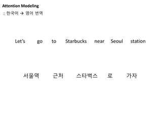
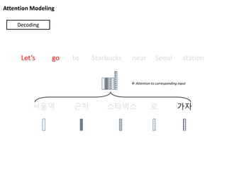
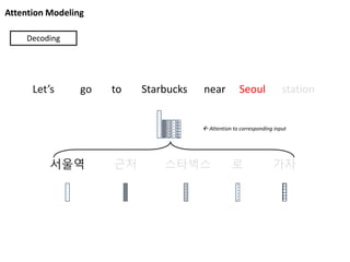
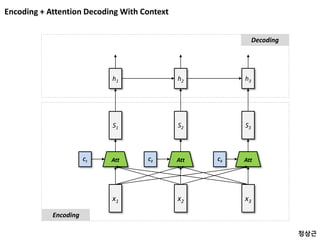
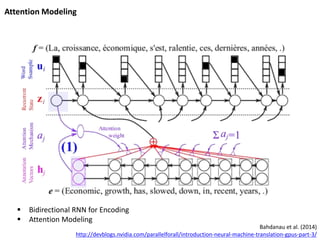
Attention Modeling
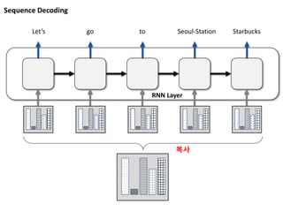
서울역 근처스타벅스 로 가자
Let’s go to Starbucks near Seoul station
Decoding
Attention to corresponding input
62.
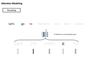
Attention Modeling
서울역 근처스타벅스 로 가자
Let’s go to Starbucks near Seoul station
Decoding
Attention to corresponding input
63.
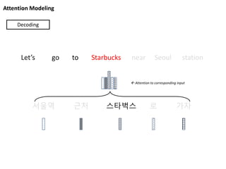
Attention Modeling
서울역 근처스타벅스 로 가자
Let’s go to Starbucks near Seoul station
Decoding
Attention to corresponding input
64.
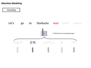
Attention Modeling
서울역 근처스타벅스 로 가자
Let’s go to Starbucks near Seoul station
Decoding
Attention to corresponding input
65.
Attention Modeling
서울역 근처스타벅스 로 가자
Let’s go to Starbucks near Seoul station
Decoding
Attention to corresponding input
66.
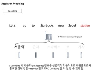
Attention Modeling
서울역 근처스타벅스 로 가자
Let’s go to Starbucks near Seoul station
Decoding
Attention to corresponding input
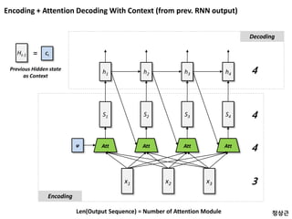
:: Decoding 시 사용되는 Encoding 정보를 선별적이고 동적으로 바꿔줌으로써
(중요한 것에 집중-Attention함으로써) Decoding 을 더 잘 할 수 있게 됨
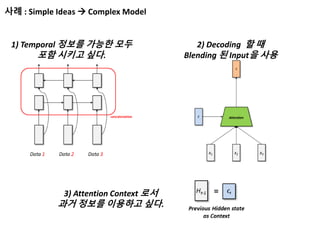
사례 : SimpleIdeas Complex Model
1) Temporal 정보를 가능한 모두
포함 시키고 싶다.
2) Decoding 할 때
Blending 된 Input을 사용
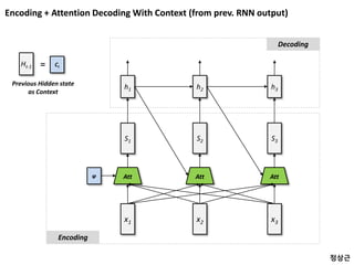
3) Attention Context 로서
과거 정보를 이용하고 싶다.
74.
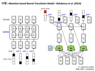
사례 : Attentionbased Neural Translation Model - Bahdanau et al. (2014)
One-Hot
BiRNN
EMB EMB EMB EMB
x1 x2 x3 x4
F1 F2 F3 F4
B1 B2 B3 B4
N1 N2 N3 N4Concat
Att
S1
Att
S2
Att
S3
φ
A A
C
h1 h2 h3
N1 N2 N3 N4
A A
Softmax
D1 D2 D2
EMB’ EMB’ EMB’
D0
EMB’
Special Symbol
A : alignment weight
EMB, EMB’ : Embedding
75.
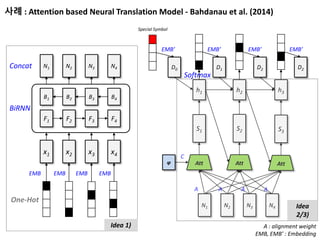
사례 : Attentionbased Neural Translation Model - Bahdanau et al. (2014)
One-Hot
BiRNN
EMB EMB EMB EMB
x1 x2 x3 x4
F1 F2 F3 F4
B1 B2 B3 B4
N1 N2 N3 N4Concat
Att
S1
Att
S2
Att
S3
φ
A A
C
h1 h2 h3
N1 N2 N3 N4
A A
Softmax
D1 D2 D2
EMB’ EMB’ EMB’
D0
EMB’
Special Symbol
A : alignment weight
EMB, EMB’ : Embedding
Idea 1)
Idea
2/3)
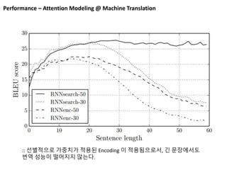
Performance – AttentionModeling @ Machine Translation
:: 선별적으로 가중치가 적용된 Encoding 이 적용됨으로서, 긴 문장에서도
번역 성능이 떨어지지 않는다.
78.
Xu et al.(2015)
Show, Attend and Tell: Neural Image Caption Generation with Visual Attention
http://devblogs.nvidia.com/parallelforall/introduction-neural-machine-translation-gpus-part-3/
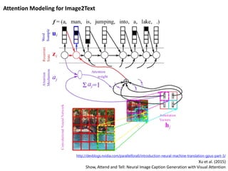
Attention Modeling for Image2Text
79.
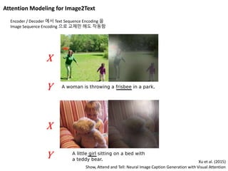
Attention Modeling forImage2Text
Xu et al. (2015)
Show, Attend and Tell: Neural Image Caption Generation with Visual Attention
Encoder / Decoder 에서 Text Sequence Encoding 을
Image Sequence Encoding 으로 교체만 해도 작동함
X
Y
X
Y
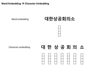
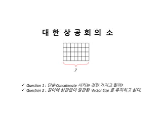
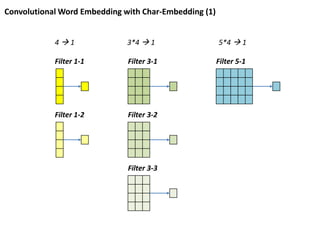
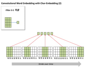
Convolutional Word Embeddingwith Char-Embedding (2)
Filter 3-1 적용
대 한 상 공 회 의 소 대 한 상 공 회 의 소 대 한 상 공 회 의 소 대 한 상 공 회 의 소 대 한 상 공 회 의 소
Stride over time
87.
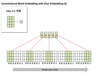
Convolutional Word Embeddingwith Char-Embedding (3)
Filter 3-2 적용
대 한 상 공 회 의 소 대 한 상 공 회 의 소 대 한 상 공 회 의 소 대 한 상 공 회 의 소 대 한 상 공 회 의 소
Stride over time
88.
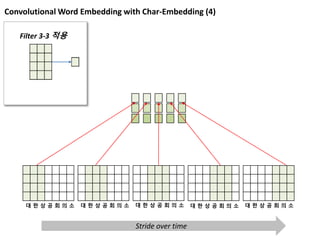
Convolutional Word Embeddingwith Char-Embedding (4)
Filter 3-3 적용
대 한 상 공 회 의 소 대 한 상 공 회 의 소 대 한 상 공 회 의 소 대 한 상 공 회 의 소 대 한 상 공 회 의 소
Stride over time
89.
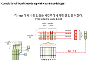
Convolutional Word Embeddingwith Char-Embedding (5)
대 한 상 공 회 의 소
take max
take max
take max
각 Filter 에서 나온 값들을 시간축에서 가장 큰 값을 취한다.
(max-pooling-over-time)
num_filter
(3)
Length – Range + 1
( 7 – 3 + 1 = 5 )
4x7 3
num_filter
(3)
90.
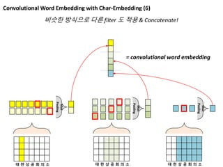
Convolutional Word Embeddingwith Char-Embedding (6)
대 한 상 공 회 의 소
비슷한 방식으로 다른 filter 도 적용 & Concatenate!
Max
Pooling
대 한 상 공 회 의 소
Max
Pooling
대 한 상 공 회 의 소
Max
Pooling
= convolutional word embedding
91.
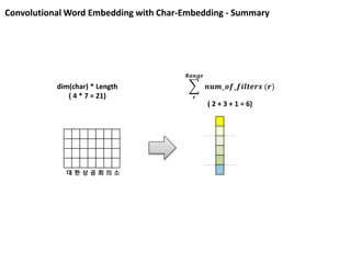
Convolutional Word Embeddingwith Char-Embedding - Summary
대 한 상 공 회 의 소
dim(char) * Length
( 4 * 7 = 21) 𝒓
𝑹𝒂𝒏𝒈𝒆
𝒏𝒖𝒎_𝒐𝒇_𝒇𝒊𝒍𝒕𝒆𝒓𝒔 (𝒓)
( 2 + 3 + 1 = 6)
92.
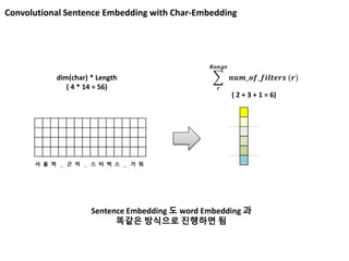
Convolutional Sentence Embeddingwith Char-Embedding
dim(char) * Length
( 4 * 14 = 56) 𝒓
𝑹𝒂𝒏𝒈𝒆
𝒏𝒖𝒎_𝒐𝒇_𝒇𝒊𝒍𝒕𝒆𝒓𝒔 (𝒓)
( 2 + 3 + 1 = 6)
서 울 역 _ 근 처 _ 스 타 벅 스 _ 가 줘
Sentence Embedding 도 word Embedding 과
똑같은 방식으로 진행하면 됨
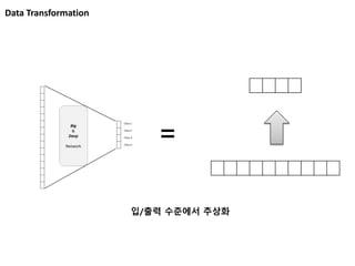
![V to 1 - Linear Algebra
Weighted Sum
w1
w2
w3
w4
w5
w6
w7
w8
w9
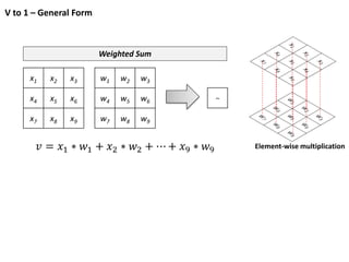
x1 x2 x3 x4 x5 x6 x7 x8 x9 X =
𝑖
9
𝑥𝑖 ∗ 𝑤𝑖
[1 x 9] matrix
[9x1] matrix
[1x1] matrix](https://image.slidesharecdn.com/multiplevectorencoding-180314024003/85/Multiple-vector-encoding-KOR-version-12-320.jpg)
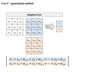
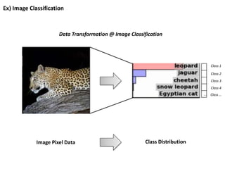
![V to V’ – Linear Algebra
Weighted Sum
w1,1
w1,2
w1,3
w1,4
w1,5
w1,6
w1,7
w1,8
w1,9
x1 x2 x3 x4 x5 x6 x7 x8 x9 X = 𝑖
9
𝑥𝑖 ∗ 𝑤1,𝑖
w2,1
w2,2
w2,3
w2,4
w2,5
w2,6
w2,7
w2,8
w2,9
[1 x 9] matrix
[9x2] matrix
𝑖
9
𝑥𝑖 ∗ 𝑤2,𝑖
,
[1x2] matrix
Fully Connected Network](https://image.slidesharecdn.com/multiplevectorencoding-180314024003/85/Multiple-vector-encoding-KOR-version-18-320.jpg)
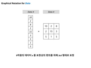
![V to V’ with Context - Linear Algebra
w1,1
w1,2
w1,3
w1,4
w1,5
w1,6
w1,7
w1,8
w1,9
x1 x2 x3 x4 x5 x6 x7 x8 x9 X = 𝑖
9
𝑥𝑖 ∗ 𝑤1,𝑖
w2,1
w2,2
w2,3
w2,4
w2,5
w2,6
w2,7
w2,8
w2,9
[1 x 9] matrix
[9x2] matrix
𝑖
9
𝑥𝑖 ∗ 𝑤2,𝑖
,
[1x2] matrix
c1 c2 c3 c4
[1 x 4] matrix wC
1,1
wC
1,2
wC
1,3
wC
1,4
wC
2,1
wC
2,2
wC
2,3
wC
2,4
= 𝑖
4
𝑐𝑖 ∗ 𝑤1,𝑖
𝑐
𝑖
4
𝑥𝑖 ∗ 𝑤2,𝑖
𝑐
,
[1x2] matrix
X
I II
I II](https://image.slidesharecdn.com/multiplevectorencoding-180314024003/85/Multiple-vector-encoding-KOR-version-22-320.jpg)
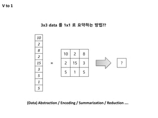
![V to V’ with Context - Linear Algebra (simple)
w1,1
w1,2
w1,3
w1,4
w1,5
w1,6
w1,7
w1,8
w1,9
x1 x2 x3 x4 x5 x6 x7 x8 x9 c1 c2 c3 c4 X =
𝑖
9
𝑥𝑖 ∗ 𝑤1,𝑖
+
𝑖
4
𝑐𝑖 ∗ 𝑤1,𝑖
𝑐
w2,1
w2,2
w2,3
w2,4
w2,5
w2,6
w2,7
w2,8
w2,9
[1 x (9+4)] matrix
[(9+4) x2] matrix
[1x2] matrix
wC
1,1
wC
1,2
wC
1,3
wC
1,4
wC
2,1
wC
2,2
wC
2,3
wC
2,4
𝑖
9
𝑥𝑖 ∗ 𝑤2,𝑖
+
𝑖
4
𝑐𝑖 ∗ 𝑤2,𝑖
𝑐
입력 Data 를 Concatenate 시키고
Weight Matrix를 하나로 만들어서 처리](https://image.slidesharecdn.com/multiplevectorencoding-180314024003/85/Multiple-vector-encoding-KOR-version-23-320.jpg)

![[참고] Translation Pyramid
Bernard Vauquois' pyramid showing comparative
depths of intermediary representation, interlingual
machine translation at the peak, followed by transfer-
based, then direct translation.
[ http://en.wikipedia.org/wiki/Machine_translation]](https://image.slidesharecdn.com/multiplevectorencoding-180314024003/85/Multiple-vector-encoding-KOR-version-45-320.jpg)

![Context 반영 방법
concat
어떻게 C 와 xi 을
조합할까?
xi
C
X W
𝑠𝑐𝑜𝑟𝑒 = 𝑣 𝑇
tanh(𝑊 𝑥𝑖; 𝑐 )
concatenate
[ 1 x (V+K) ] [ (V+K) x M ]
K
V
X VT
[ M x 1 ]
[ 1 x M ]
general
xi
XWC X
[ 1 x K ] [ K x V ] [ V x 1]
1
1
𝑠𝑐𝑜𝑟𝑒 = 𝑐𝑊𝑥𝑖
𝑇
dot
xi
C X
[ 1 x K ] [ V x 1 ]
1
!!! K = V 일때만 가능
V+K M 1
Minh-Thang et al., “Effective Approaches to Attention-based Neural Machine Translation”
𝑠𝑐𝑜𝑟𝑒 = 𝑐𝑥𝑖
𝑇](https://image.slidesharecdn.com/multiplevectorencoding-180314024003/85/Multiple-vector-encoding-KOR-version-58-320.jpg)
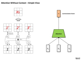
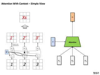
![[Review] Attention With Context – Simple View
x1 x2 x3
Attention
Xs
C
정상근](https://image.slidesharecdn.com/multiplevectorencoding-180314024003/85/Multiple-vector-encoding-KOR-version-67-320.jpg)


![[신경망기초] 심층신경망개요](https://cdn.slidesharecdn.com/ss_thumbnails/nn10-180318142325-thumbnail.jpg?width=640&height=640&fit=bounds)


![[기초개념] Graph Convolutional Network (GCN)](https://cdn.slidesharecdn.com/ss_thumbnails/agistdkimgcn190507-190507153736-thumbnail.jpg?width=640&height=640&fit=bounds)


