Minimum Spanning Trees2
Outline and Reading
Minimum Spanning Trees (§12.7)
Definitions
A crucial fact
The Prim-Jarnik Algorithm (§12.7.2)
Kruskal's Algorithm (§12.7.1)
Baruvka's Algorithm
3.
Minimum Spanning Trees3
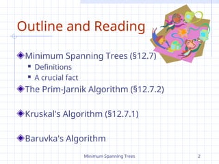
Minimum Spanning Tree
Spanning subgraph
Subgraph of a graph G
containing all the vertices of
G
Spanning tree
Spanning subgraph that is
itself a (free) tree
Minimum spanning tree (MST)
Spanning tree of a weighted
graph with minimum total
edge weight
Applications
Communications networks
Transportation networks
ORD
PIT
ATL
STL
DEN
DFW
DCA
10
1
9
8
6
3
2
5
7
4
4.
Minimum Spanning Trees4
Cycle Property
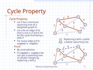
Cycle Property:
Let T be a minimum
spanning tree of a
weighted graph G
Let e be an edge of G
that is not in T and C let
be the cycle formed by e
with T
For every edge f of C,
weight(f) weight(e)
Proof:
By contradiction
If weight(f) weight(e) we
can get a spanning tree
of smaller weight by
replacing e with f
8
4
2
3
6
7
7
9
8
e
C
f
8
4
2
3
6
7
7
9
8
C
e
f
Replacing f with e yields
a better spanning tree
5.
Minimum Spanning Trees5
U V
Partition Property
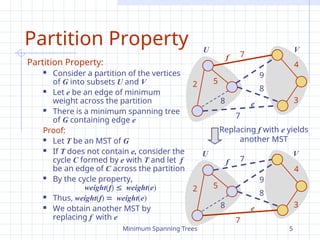
Partition Property:
Consider a partition of the vertices
of G into subsets U and V
Let e be an edge of minimum
weight across the partition
There is a minimum spanning tree
of G containing edge e
Proof:
Let T be an MST of G
If T does not contain e, consider the
cycle C formed by e with T and let f
be an edge of C across the partition
By the cycle property,
weight(f) weight(e)
Thus, weight(f) weight(e)
We obtain another MST by
replacing f with e
7
4
2
8
5
7
3
9
8 e
f
7
4
2
8
5
7
3
9
8 e
f
Replacing f with e yields
another MST
U V
6.
Minimum Spanning Trees6
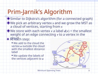
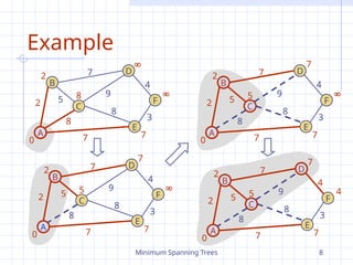
Prim-Jarnik’s Algorithm
Similar to Dijkstra’s algorithm (for a connected graph)
We pick an arbitrary vertex s and we grow the MST as
a cloud of vertices, starting from s
We store with each vertex v a label d(v) = the smallest
weight of an edge connecting v to a vertex in the
cloud
At each step:
We add to the cloud the
vertex u outside the cloud
with the smallest distance
label
We update the labels of
the vertices adjacent to u
7.
Minimum Spanning Trees7
Prim-Jarnik’s Algorithm
(cont.)
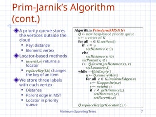
A priority queue stores
the vertices outside the
cloud
Key: distance
Element: vertex
Locator-based methods
insert(k,e) returns a
locator
replaceKey(l,k) changes
the key of an item
We store three labels
with each vertex:
Distance
Parent edge in MST
Locator in priority
queue
Algorithm PrimJarnikMST(G)
Q new heap-based priority queue
s a vertex of G
for all v G.vertices()
if v s
setDistance(v, 0)
else
setDistance(v, )
setParent(v, )
l Q.insert(getDistance(v), v)
setLocator(v,l)
while Q.isEmpty()
u Q.removeMin()
for all e G.incidentEdges(u)
z G.opposite(u,e)
r weight(e)
if r getDistance(z)
setDistance(z,r)
setParent(z,e)
Q.replaceKey(getLocator(z),r)
8.
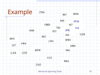
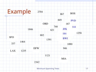
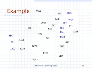
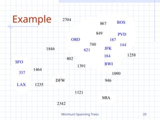
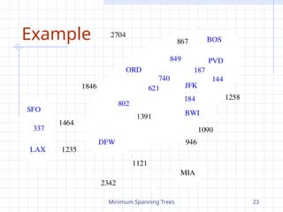
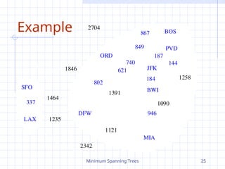
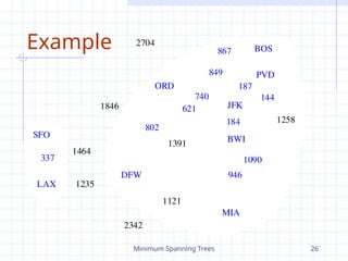
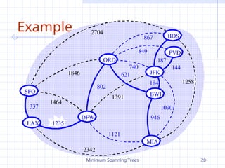
Minimum Spanning Trees8
Example
B
D
C
A
F
E
7
4
2
8
5
7
3
9
8
0
7
2
8
B
D
C
A
F
E
7
4
2
8
5
7
3
9
8
0
7
2
5
7
B
D
C
A
F
E
7
4
2
8
5
7
3
9
8
0
7
2
5
7
B
D
C
A
F
E
7
4
2
8
5
7
3
9
8
0
7
2
5 4
7
9.
Minimum Spanning Trees9
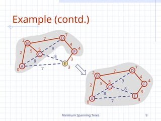
Example (contd.)
B
D
C
A
F
E
7
4
2
8
5
7
3
9
8
0
3
2
5 4
7
B
D
C
A
F
E
7
4
2
8
5
7
3
9
8
0
3
2
5 4
7
10.
Minimum Spanning Trees10
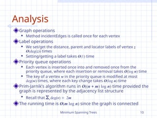
Analysis
Graph operations
Method incidentEdges is called once for each vertex
Label operations
We set/get the distance, parent and locator labels of vertex z
O(deg(z)) times
Setting/getting a label takes O(1) time
Priority queue operations
Each vertex is inserted once into and removed once from the
priority queue, where each insertion or removal takes O(log n) time
The key of a vertex w in the priority queue is modified at most
deg(w) times, where each key change takes O(log n) time
Prim-Jarnik’s algorithm runs in O((n m) log n) time provided the
graph is represented by the adjacency list structure
Recall that v deg(v) 2m
The running time is O(m log n) since the graph is connected
11.
Minimum Spanning Trees11
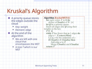
Kruskal’s Algorithm
A priority queue stores
the edges outside the
cloud
Key: weight
Element: edge
At the end of the
algorithm
We are left with one
cloud that
encompasses the MST
A tree T which is our
MST
Algorithm KruskalMST(G)
for each vertex V in G do
define a Cloud(v) of {v}
let Q be a priority queue.
Insert all edges into Q using their
weights as the key
T
while T has fewer than n-1 edges do
edge e = T.removeMin()
Let u, v be the endpoints of e
if Cloud(v) Cloud(u) then
Add edge e to T
Merge Cloud(v) and Cloud(u)
return T
12.
Minimum Spanning Trees12
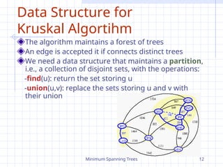
Data Structure for
Kruskal Algortihm
The algorithm maintains a forest of trees
An edge is accepted it if connects distinct trees
We need a data structure that maintains a partition,
i.e., a collection of disjoint sets, with the operations:
-find(u): return the set storing u
-union(u,v): replace the sets storing u and v with
their union
13.
Minimum Spanning Trees13
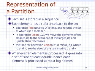
Representation of
a Partition
Each set is stored in a sequence
Each element has a reference back to the set
operation find(u) takes O(1) time, and returns the set
of which u is a member.
in operation union(u,v), we move the elements of the
smaller set to the sequence of the larger set and
update their references
the time for operation union(u,v) is min(nu,nv), where
nu and nv are the sizes of the sets storing u and v
Whenever an element is processed, it goes into
a set of size at least double, hence each
element is processed at most log n times
14.
Minimum Spanning Trees14
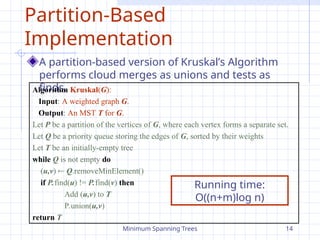
Partition-Based
Implementation
A partition-based version of Kruskal’s Algorithm
performs cloud merges as unions and tests as
finds.
Algorithm Kruskal(G):
Input: A weighted graph G.
Output: An MST T for G.
Let P be a partition of the vertices of G, where each vertex forms a separate set.
Let Q be a priority queue storing the edges of G, sorted by their weights
Let T be an initially-empty tree
while Q is not empty do
(u,v) Q.removeMinElement()
if P.find(u) != P.find(v) then
Add (u,v) to T
P.union(u,v)
return T
Running time:
O((n+m)log n)
Minimum Spanning Trees29
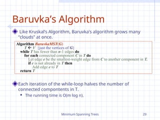
Baruvka’s Algorithm
Like Kruskal’s Algorithm, Baruvka’s algorithm grows many
“clouds” at once.
Each iteration of the while-loop halves the number of
connected compontents in T.
The running time is O(m log n).
Algorithm BaruvkaMST(G)
T V {just the vertices of G}
while T has fewer than n-1 edges do
for each connected component C in T do
Let edge e be the smallest-weight edge from C to another component in T.
if e is not already in T then
Add edge e to T
return T


![DAA-seminar-1[1].pptx Design and Analysis Of The Algorithm](https://cdn.slidesharecdn.com/ss_thumbnails/daa-seminar-11-250921155526-8ea0ea04-thumbnail.jpg?width=640&height=640&fit=bounds)