[8] implementation of pmsm servo drive using digital signal processing
MSSISS ATLAS
1. Development of a Realtime Prediction Model of Driver Behavior
at Intersections Using Kinematic Time Series Data
Yaoyaun Vincent Tana
†, Michael Elliotta,b
, Carol Flannaganc
aUniversity of Michigan Department of Biostatistics, bInstitute for Social Research cUniversity of Michigan Transportation Research Institute
Introduction
An autonomous vehicle is a vehicle where no human supervision or driving
is needed, for example the Google Driverless Car. As these vehicles en-
ter the fleet, they will have to interact with human drivers. One challenge
these vehicles will face is that human drivers do not always communicate
their decisions well. For example, a driver will not indicate whether they
will stop before executing a turn. Fortunately, the kinematic behavior of the
driver’s vehicle may provide enough information to make a good predic-
tion of driver intent within a short timeframe. We developed a prediction
model by analyzing the kinematic behavior, i.e. speed, of 108 drivers from
a naturalistic driving study (Sayer et. al., 2011). We narrowed our ob-
jective to the prediction of whether a driver would stop before executing a
left turn. We used Principal Components Analysis (PCA) to generate inde-
pendent variables that explain the variation in vehicle speed before a turn.
Using Bayesian Additive Regression Trees (BART) (Chipman et.al., 2010)
we linked our PCA scores to whether a driver would stop before executing
a left turn. Preliminary results suggest that speed of a vehicle can predict
whether a driver would stop. Once our model is fully developed, we believe
it would be extendable to other forms of driver behavior prediction.
Data
• Data collected between April 2009 and May 2010.
• 108 licensed drivers from Michigan.
• 40 days of driving per driver: 12-day baseline unsupervised driving, 28-
day driving with safety systems activated.
• 3,795 turns.
• 1,823 left turns (our primary focus) from 108 drivers.
Variables used:
• Time at −100m away from center of intersection, our reference start for
each turn.
• Time (10 millisecond interval)
• Speed (m/s) – Time series.
• Realtime Distance (m) – Time series.
Switching from time-series to ‘distance’-series
Because vehicles approach intersections at varying speeds, the duration of
every left turn was different. To obtain a rectangular data structure, we
switched to a ‘distance’-series where data, speed in our context, would be
recorded at every 1 meter (m) interval. To transform speed at every 10
millisecond to speed at every 1m interval, we first determined the realtime
distance closest to every 1m interval from our reference start. We denote
this realtime distance as dij where i is the ith turn and j is the jth meter
interval, j = −100, . . . , −1. We then take the speed at dij as the speed at
the jth meter interval. If there were ties in dij, we took the average of their
speeds. Finally, we restricted our distance-series from -100m to -1m away
from the center of intersection.
Time-varying binary outcome: left-turn pre-stop
Our time-varying binary outcome was defined as:
• 0 (did not stop) throughout – if the speed was >1m/s for −100m to −1m
from the center of intersection.
• If the speed decreased to ≤1m/s within −100m to −1m, the outcome from
−100m till the last jthm the turn speed decreased to <1m/s was coded as
1 (stopped). Subsequent outcomes from j + 1thm till −1m were coded as
0 (did not stop).
Method
Moving window
Let Yij be the outcome and Xij be the speed of the ith
turn at
the jth
m, j = −100, . . . , −1. Our objective was to use current
and past speed to predict a pre-turn stop. We felt that recent
speeds would provide better information compared to full past
speeds. We confirmed this by comparing Area Under the Curve
(AUC) results which are not presented here. We defined recent
speeds using a moving window of 10m where at any jth
m from
the center of intersection, j = −90, . . . , −1, the 10 most recent
speeds including the current speed would be used for predic-
tion.
Principal Components Analysis
We used PCA to summarize information from the 10 speed en-
tries at each jth
m i.e. we determined the vector δi such that
max
{δ:||δ||=1}
V ar(δT
i Xi) would be achieved.
Bayesian Additive Regression Tree
We then used BART to relate the PCA scores to our outcomes
at each jth
m. We chose BART because it is a non-linear method
that handles interaction terms naturally. We defined BART as
Yij =
m
j=1
g(δT
i Xi; Tij, Mij) + i, i ∼ N(0, σ2
).
We used default BART because it is computationally less in-
tense and still achieves acceptable results in many settings.
Prediction evaluation
We plotted the distribution of the predicted stopping probabil-
ities for stoppers and non-stoppers, Receiver Operating Curve
(ROC), and Local Polynomial Regression Fitting smoothed Pre-
cision Recall (PR) curves. In addition, we plotted the profile of
the Capture Ratio (CR) and False Discovery Ratio (FDR) at
different prediction cut-offs from 10 − 90%.
CR = True positive
True positive+False negative,
FDR = False positive
True positive+False positive.
Results
The trends for the first 3 Principal Components (PCs) from
−91m to −11m appeared stable (Figure 1). The first 3 PCs
explained at least 99% of the variation in speed before a turn.
We observed that the PCs exhibited similar trends (See Figure
1) regardless of whether recent speeds or all past speeds were
used. Similar trends persisted when we switched to a time-
based speed series (Results not shown here).
We found that the 1st
PC resembled the average speed with a
slight variation where higher weights were placed on the ear-
lier speeds far from the intersection and later speeds close to the
intersection. The 2nd
PC resembled the acceleration of the ve-
hicle since PCA weights for recent speeds were positive while
PCA weights for earlier speeds were negative. The direction of
the signs for the weights switched as the vehicle approached an
intersection, measuring deceleration.
We included the 3rd
PCs in our model because they provided
substantial AUC gains (results not shown here). In addition,
the speed profiles with high and low 3rd
PCA scores were more
consistent compared to higher ordered PCs.
Figure 1: Principal component (PC) weightings for the 1st, 2nd, and 3rd PC
at −100m to −91m, −80m to −71m, −60m to −51m, −40m to −31m, and
−20m to −11m.
−100 −94
0.09900.1000
99.48%
Distance (m)
1stPCAloadings
−80 −74
0.0970.0990.101
99.52%
Distance (m)
−60 −54
0.0970.0990.101
99.3%
Distance (m)
−40 −34
0.09800.09950.1010
99.01%
Distance (m)
−20 −14
0.0970.0990.101
97.75%
Distance (m)
−100 −94
−2001020
0.47%
Distance (m)
2ndPCAloadings
−80 −74
−505
0.44%
Distance (m)
−60 −54
−505
0.63%
Distance (m)
−40 −34
−15−5515
0.88%
Distance (m)
−20 −14
−15−5510
2%
Distance (m)
−100 −94
−100050
0.03%
Distance (m)
3rdPCAloadings
−80 −74
−100050100
0.03%
Distance (m)
−60 −54
−2000200400
0.04%
Distance (m)
−40 −34
−2002040
0.06%
Distance (m)
−20 −14
−2001020
0.16%
Distance (m)
Figure 2: Receiver Operating Curve (ROC) and Precision Recall (PR) curve
of the moving window Principal Component Analysis Bayesian Additive
Regression Tree model at −100m to −91m, −80m to −71m, −60m to −51m,
−40m to −31m, and −20m to −11m.
0.0 0.6
0.00.20.40.60.81.0
−91m
False Positive Rate
(ROC)TruePositiveRate
0.0 0.6
0.00.20.40.60.81.0
−71m
False Positive Rate
0.0 0.6
0.00.20.40.60.81.0
−51m
False Positive Rate
0.0 0.6
0.00.20.40.60.81.0
−31m
False Positive Rate
0.0 0.6
0.00.20.40.60.81.0
−11m
False Positive Rate
0.0 0.6
0.30.40.50.60.70.80.91.0
Recall
(PR)Precision
0.0 0.6
0.30.40.50.60.70.80.91.0
Recall
0.0 0.6
0.30.40.50.60.70.80.91.0
Recall
0.0 0.6
0.30.40.50.60.70.80.91.0
Recall
0.0 0.6
0.30.40.50.60.70.80.91.0
Recall
Figure 3: Distribution of predicted stopping probabilities for stoppers and
non-stoppers at −100m to −91m, −80m to −71m, −60m to −51m, −40m
to −31m, and −20m to −11m.
0.0 0.6
0.00.51.01.52.02.5
−91m
Probabilities
Stoppersdensity
0.0 0.6
0.00.51.01.5
−71m
Probabilities
0.0 0.6
0.00.51.01.52.0
−51m
Probabilities
0.0 0.6
0.00.51.01.5
−31m
Probabilities
0.0 0.6
0.00.51.01.52.0
−11m
Probabilities
0.0 0.6
0.00.51.01.52.02.53.0
Probabilities
Non−stoppersdensity
0.0 0.6
0.00.51.01.52.02.5
Probabilities
0.0 0.6
0.00.51.01.52.02.53.0
Probabilities
0.0 0.6
01234
Probabilities
0.0 0.6
0246810
Probabilities
Figure 4: Capture Ratio (CR) and False Discovery Ratio (FDR) at every 1m
interval from −90m to −1m for probability cut-offs: 10-90%.
−80 −60 −40 −20 0
0.00.40.8
10% cut−off
Distance (m)
Proportion
CR
FDR
−80 −60 −40 −20 0
0.00.40.8
20% cut−off
Distance (m)
CR
FDR
−80 −60 −40 −20 0
0.00.40.8
30% cut−off
Distance (m)
CR
FDR
−80 −60 −40 −20 0
0.00.40.8
40% cut−off
Distance (m)
Proportion
CR
FDR
−80 −60 −40 −20 0
0.00.40.8
50% cut−off
Distance (m)
CR
FDR
−80 −60 −40 −20 0
0.00.40.8
60% cut−off
Distance (m)
CR
FDR
−80 −60 −40 −20 0
0.00.40.8
70% cut−off
Distance (m)
Proportion
CR
FDR
−80 −60 −40 −20 0
0.00.40.8
80% cut−off
Distance (m)
CR
FDR
−80 −60 −40 −20 0
0.00.40.8
90% cut−off
Distance (m)
CR
FDR
The ROC and smoothed PR curves suggested improved pre-
dictive performance of our model as a vehicle approached the
center of an intersection (Figure 2).
We also observed higher predicted stopping probabilities for
stoppers and lower predicted probabilities for non-stoppers as
their vehicles approached the center of intersection (Figure 3).
Finally, the CR and FDR profiles (Figure 4) suggested that cut-
off probabilities from 20 to 30% provided a good balance be-
tween CR (high > 70%) and FDR (low < 60%).
Discussion
We restricted our analysis to recent speeds by using a moving
window of length 10 and summarized our data by using PCA.
We used BART to link the PCA scores to our time-varying bi-
nary outcomes using BART. Our model achieved an AUC of
0.9 by −40m away from the center of the intersection. In ad-
dition, by using a probability cut-off of 30%, we were able to
reduce our FDR to 40% while maintaining a high CR of 80%.
Limitations/Future direction
• Different drivers, intersection types, and safety system activation – Our
current analysis assumed that each turn was independent from each other.
However, similar drivers, intersection types, and safety system activation
suggest that there should be some correlation structure in our data.
• Joint modeling – we envision the use of joint modeling to incorporate
these different correlation structures together efficiently.
• Moving window length – We plan to address this issue in our joint mod-
eling setup.
• Other covariates – Other baseline covariates in the original dataset may
help us improve our prediction performance. An example is the presence
of leading vehicles.
References
• Chipman, H.A., George, E.I., McCulloch, R.E. (2010). BART: Bayesian Additive Regression Trees. The
Annals of Applied Statistics, 4(1):266-298.
• Sayer, J.R., Bogard, S.E., Buonarosa, M.L., LeBlanc, D.J., Funkhouser, D.S., Bao,S., et al. (2011). Inte-
grated vehicle-based safety systems light-vehicle field operational test key findings report. Final Report
No. DOT HS 811 416, Ann Arbor, MI: U.S. Department of Transportation, Research and Innovative
Technology Administration, ITS Joint Program Office.
Acknowledgments
This work was supported jointly by Dr. Michael Elliott and an ATLAS Research Excellence Program project
awarded to Dr. Carol Flannagan. We would also like to thank Kirsten Herold from SPH Writing Lab for the
suggestions on writing.
†Email:vincetan@umich.edu