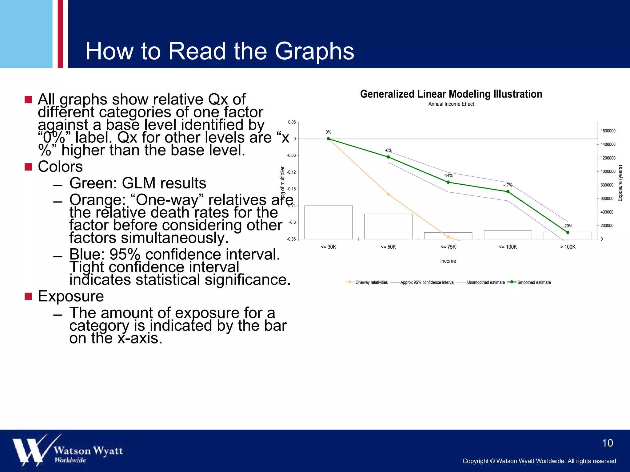
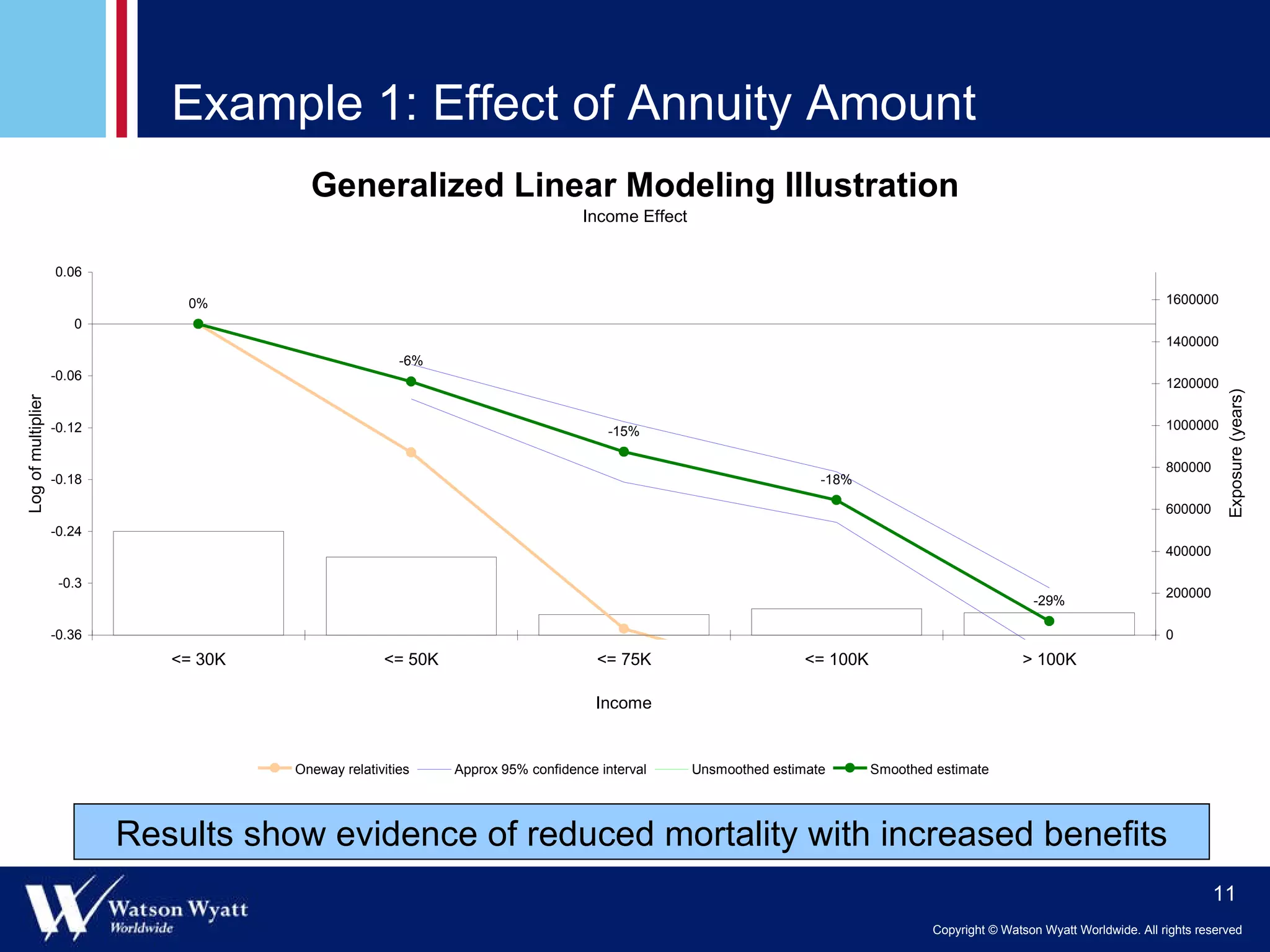
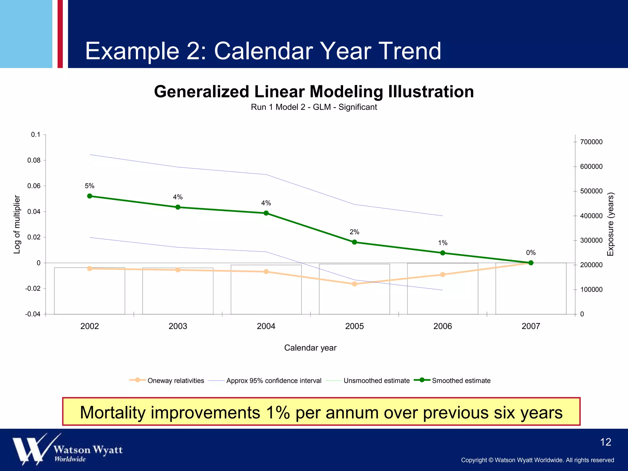
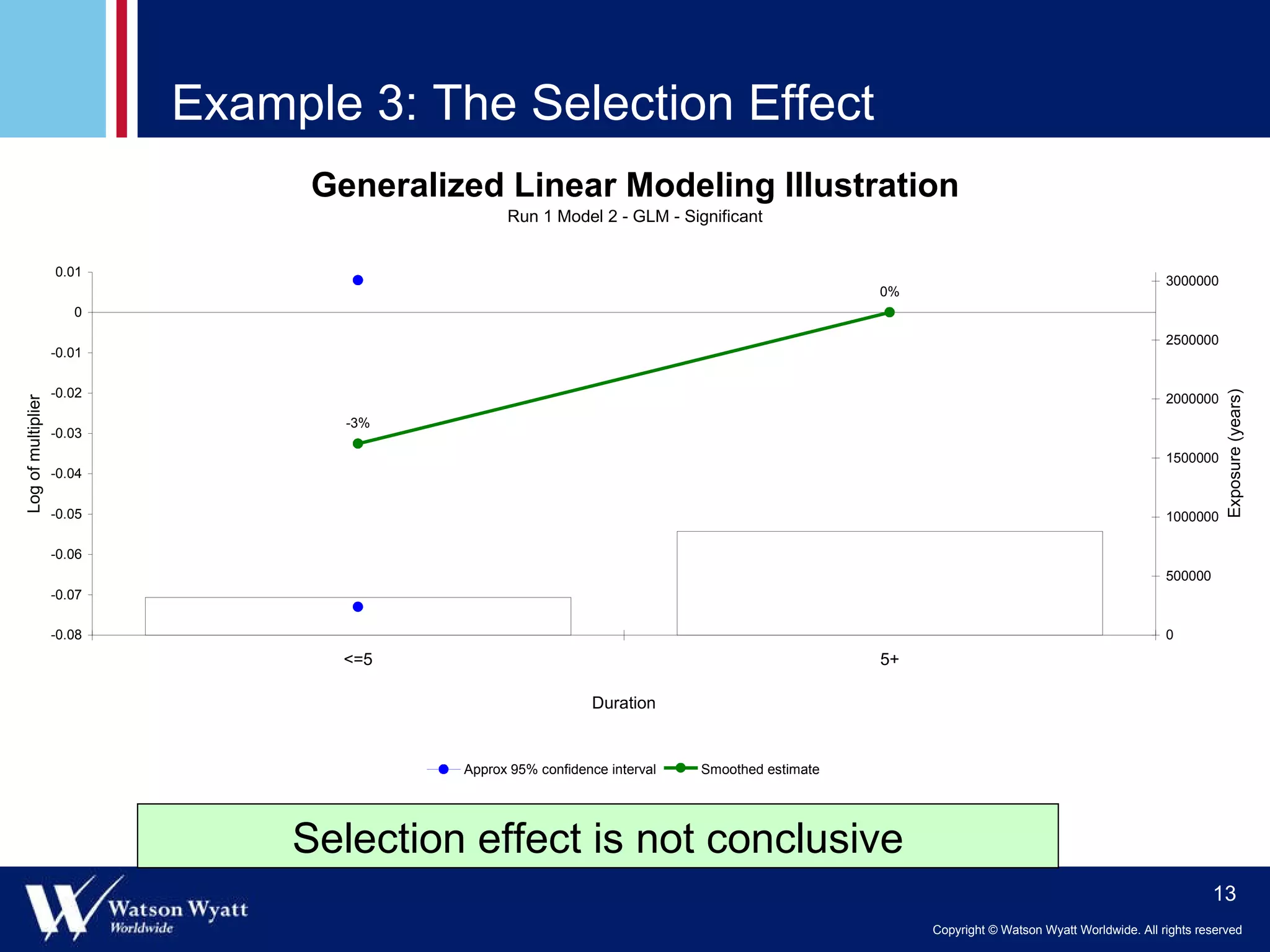
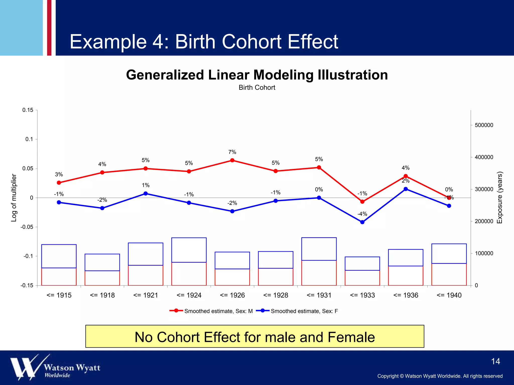
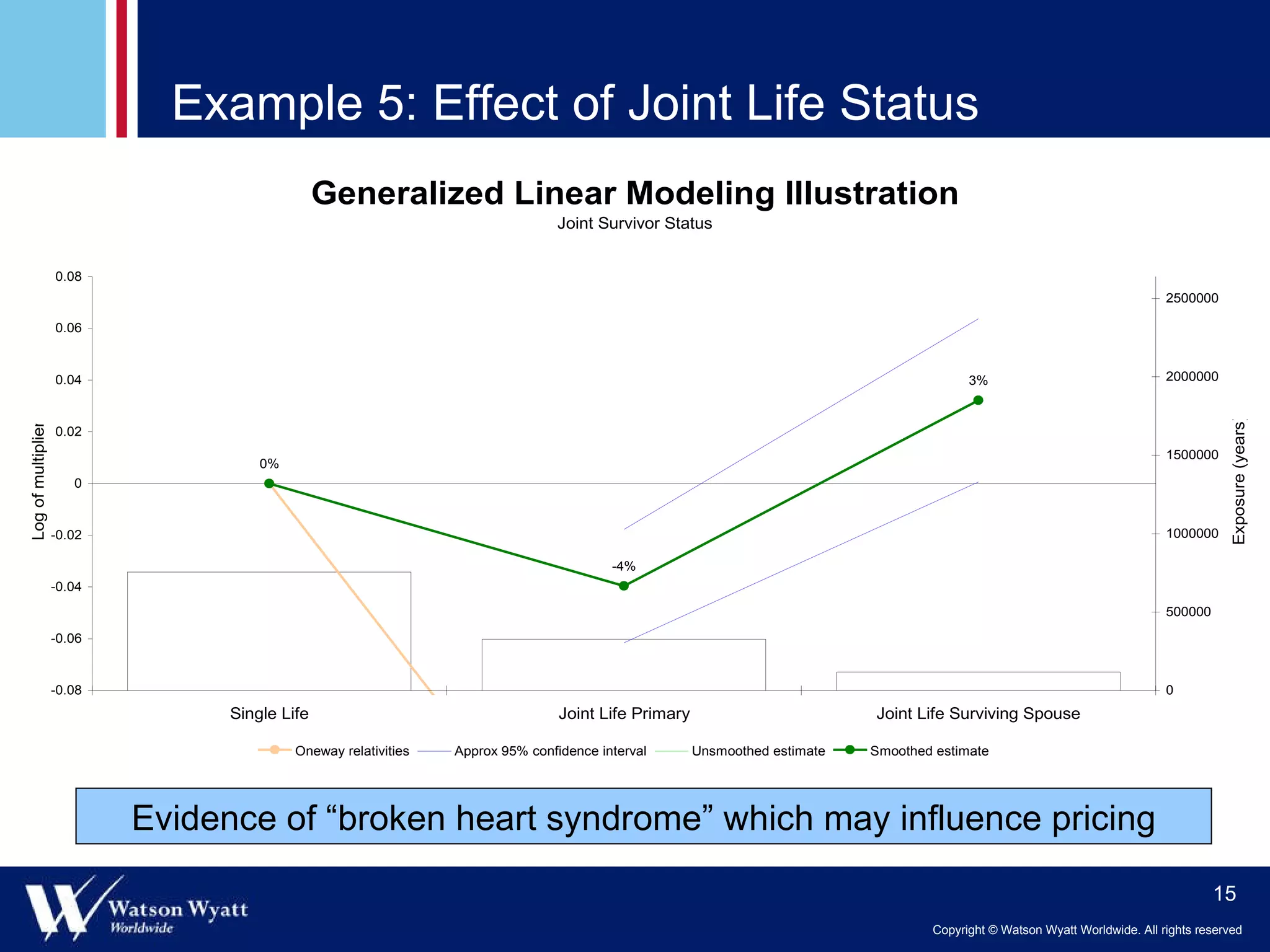
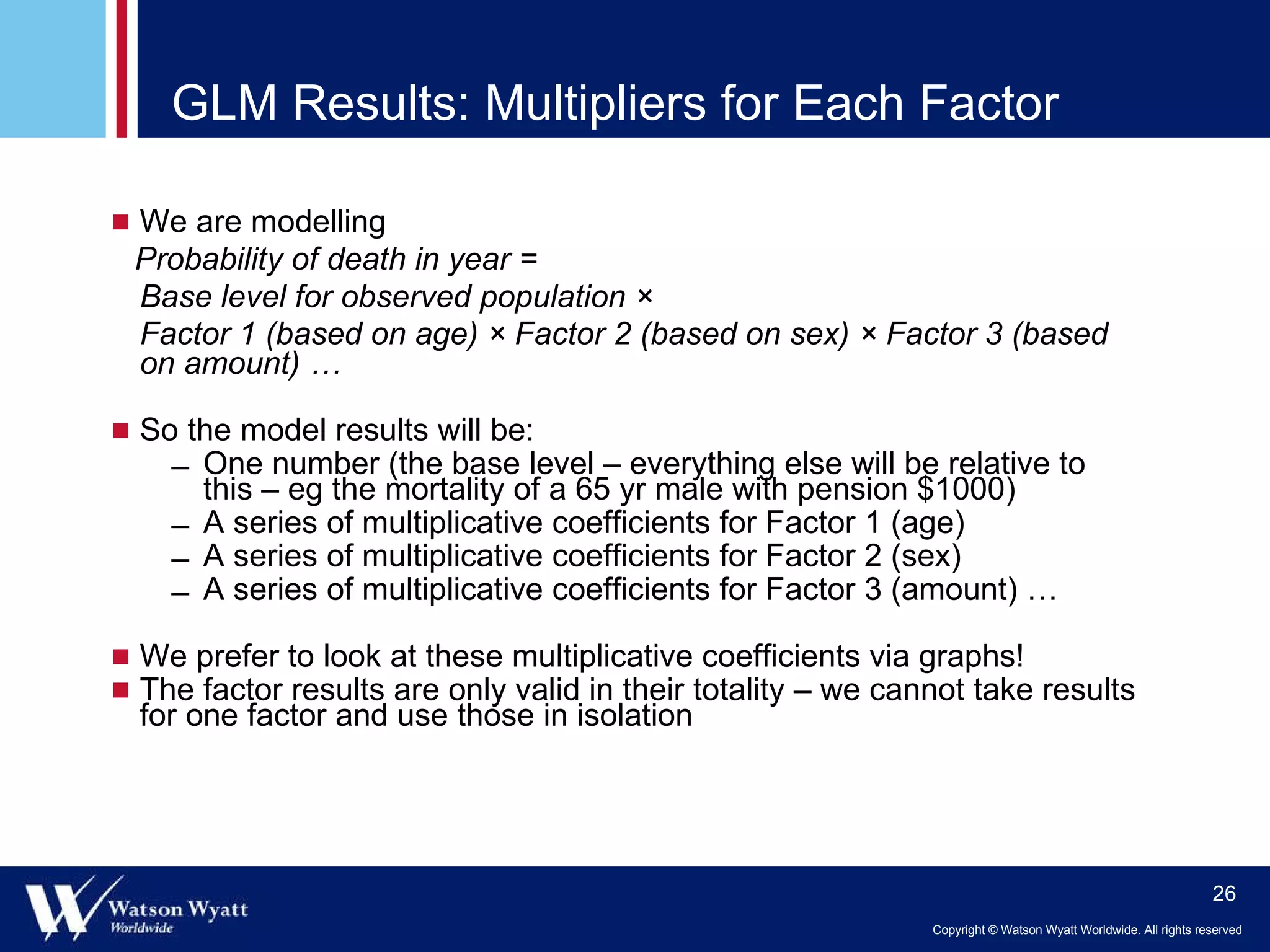
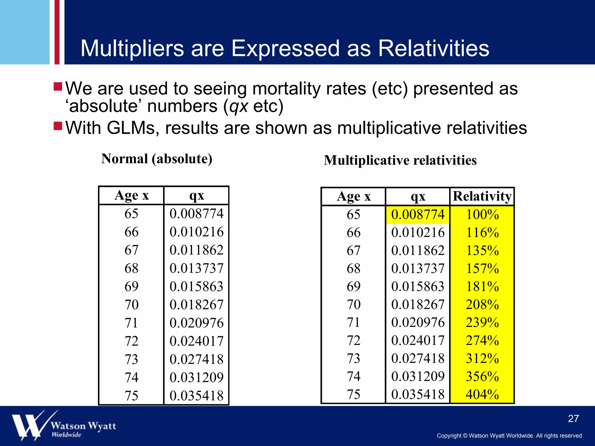
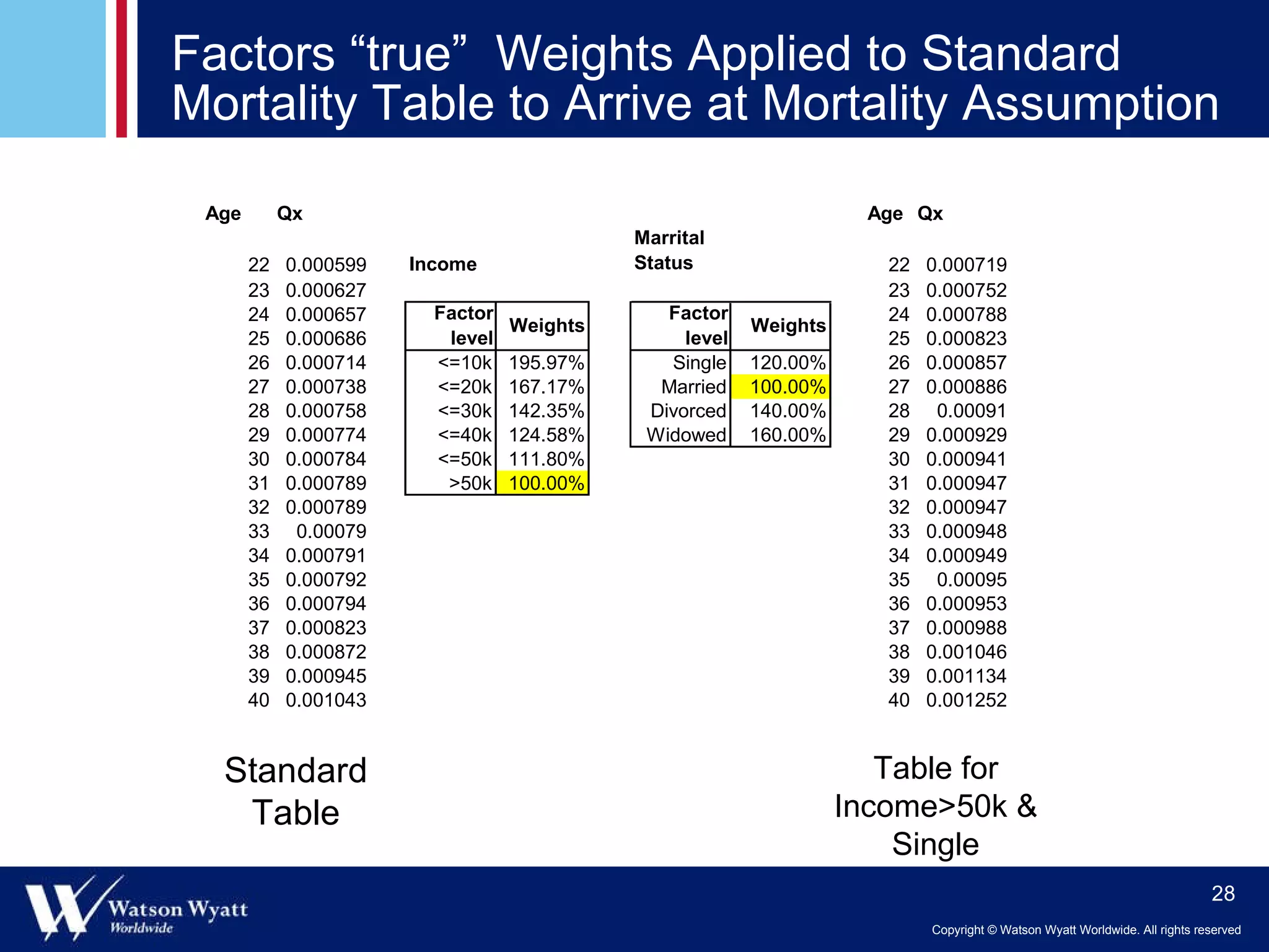
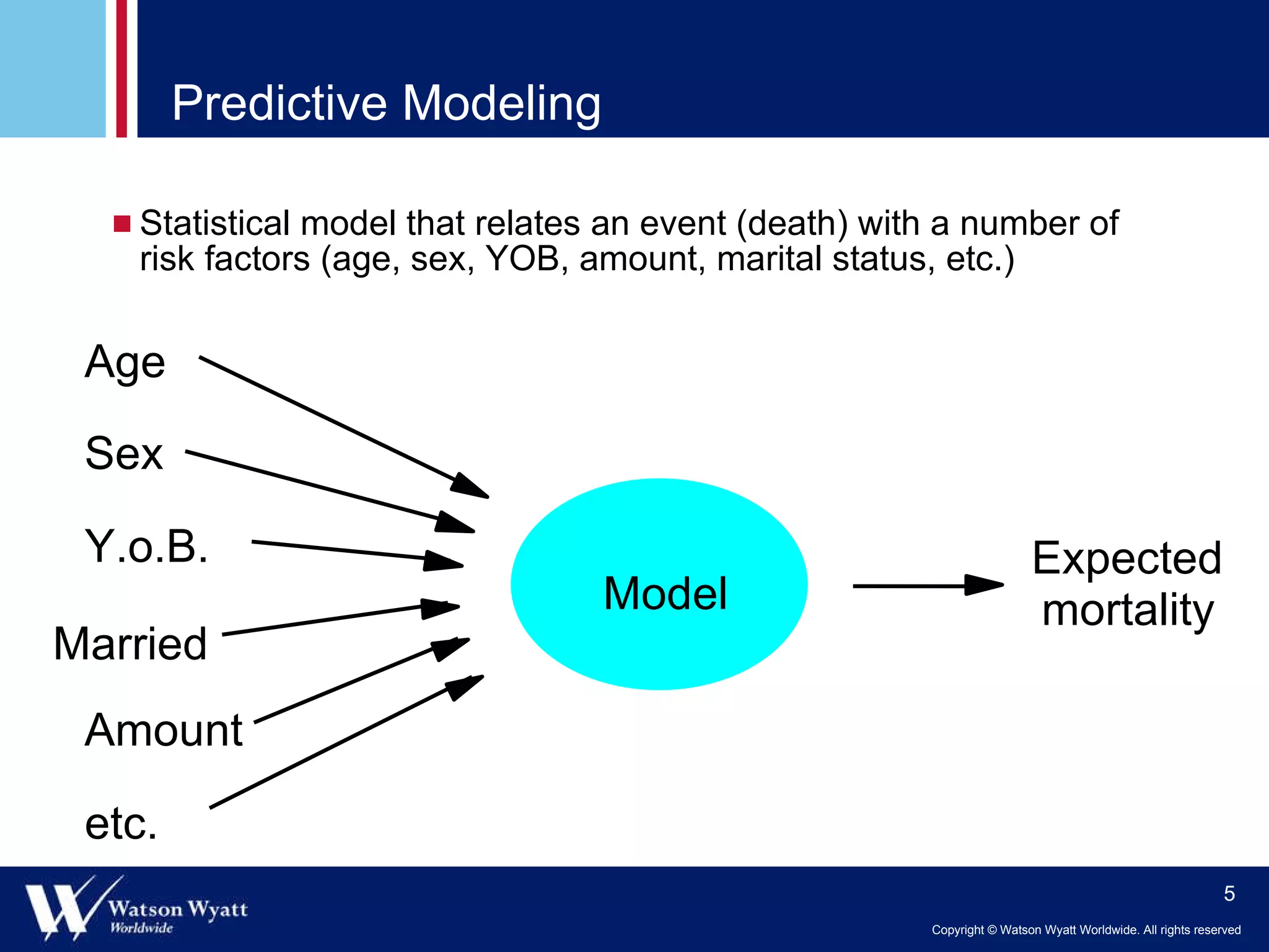
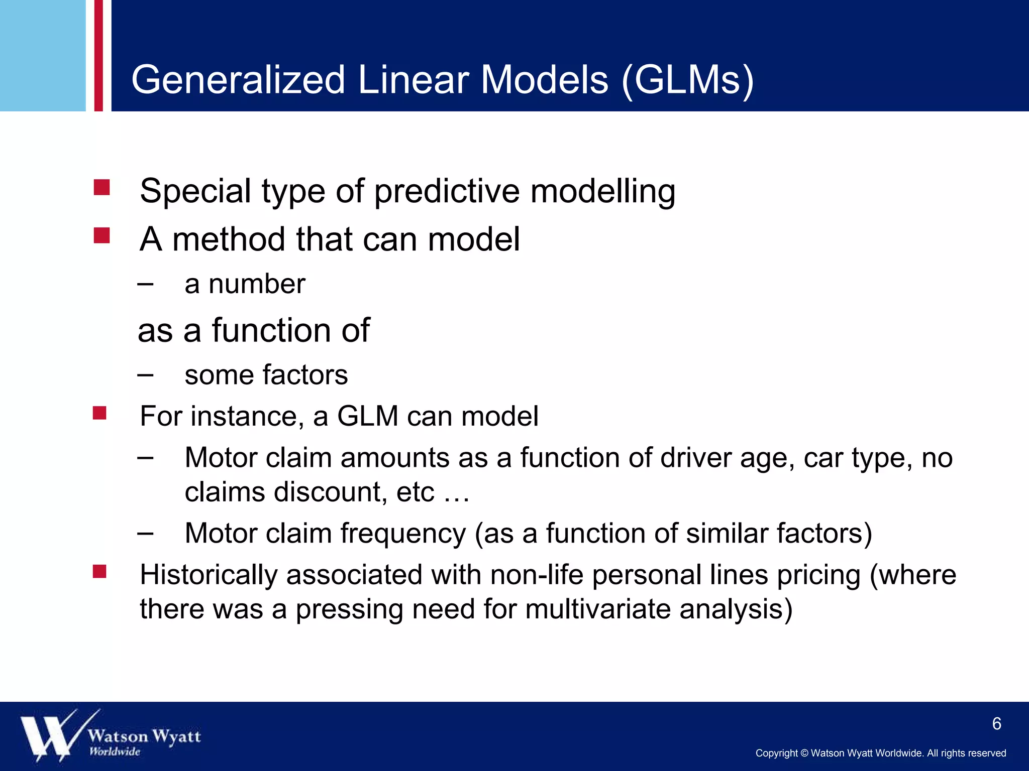
The document summarizes a presentation on modeling annuitant mortality using generalized linear models (GLMs). It discusses measuring current mortality experience, developing mortality improvement trends, and examples of GLM analyses showing the effects of factors like annuity amount, calendar year, joint life status, and birth cohort on mortality. Predictive modeling techniques from property and casualty are applied to better understand the "true" influence of multiple risk factors on mortality simultaneously.

1. 2008 Product Development Actuary Symposium The Changing Face and Pace of Mortality: An Enlightened View of Annuitant Mortality Yuhong (Jason) Xue , FSA, MAAA May 5, 2008

2. Agenda Measurement of Current Mortality Experience Apply predictive modeling techniques currently used in the P&C industry Development of Mortality Improvement Trend Advanced mathematical models to project future trends based on historical trends of mortality improvement

3. Measurement of Current Mortality Experience

4. Current Approach (Experience Study) Focus on limited risk factors that impact mortality Age, Sex, may extend to other factors (i.e. amount, marital status, and geographical location) Calculate A/E ratio with slicing and dicing techniques to come up with a set of weights (or multipliers) for each factor to be applied to a basic age/sex table Limitations Mortality is simultaneously impacted by all risk factors and has to be analyzed with all factors together “ true” weights for a factor are influences by that factor alone, assuming all else equal Fails to capture the “true” weights for each factor Calls for more sophisticated mathematical approach

5. Predictive Modeling Statistical model that relates an event (death) with a number of risk factors (age, sex, YOB, amount, marital status, etc.) Amount Y.o.B. Age etc. Sex Married Expected mortality Model

6. Generalized Linear Models (GLMs) Special type of predictive modelling A method that can model a number as a function of some factors For instance, a GLM can model Motor claim amounts as a function of driver age, car type, no claims discount, etc … Motor claim frequency (as a function of similar factors) Historically associated with non-life personal lines pricing (where there was a pressing need for multivariate analysis)

7. E[ Y ] =  = g ( X   ) -1 Observed thing (data) Some function (user defined) Some matrix based on data (user defined) as per linear models Parameters to be estimated (the answer!) Generalised linear models

8. Bedtime reading CAS 2004 Discussion Paper Programme Copies available at www.watsonwyatt.com/glm

9. Examples Examples Using GLMs to Analyze Annuitant Mortality Based on a test dataset created to simulate a typical company’s portfolio of retirees currently receiving benefits Results are merely for illustration purposes

10. How to Read the Graphs All graphs show relative Qx of different categories of one factor against a base level identified by “0%” label. Qx for other levels are “x%” higher than the base level. Colors Green: GLM results Orange: “One-way” relatives are the relative death rates for the factor before considering other factors simultaneously. Blue: 95% confidence interval . Tight confidence interval indicates statistical significance. Exposure The amount of exposure for a category is indicated by the bar on the x-axis.

11. Example 1: Effect of Annuity Amount Results show evidence of reduced mortality with increased benefits

12. Example 2: Calendar Year Trend Mortality improvements 1% per annum over previous six years

13. Example 3: The Selection Effect Selection effect is not conclusive

14. Example 4: Birth Cohort Effect No Cohort Effect for male and Female

15. Example 5: Effect of Joint Life Status Evidence of “broken heart syndrome” which may influence pricing

16. Questions we wish to answer How do different factors influence mortality? What is the cohort effect in my portfolio? What trends are there? How can I be sure of an accurate portfolio cash flow valuation?

17. Development of Mortality Improvement Trend

18. Introduction Current demographic trends should lead to accelerating growth in payout annuities Aging population Longevity Potential rates of mortality improvement are key drivers in the profitability of this business Current industry experience of mortality improvement is limited and dated

19. The Potential Impact of Longevity General Perception that investment assumption more critical than mortality Consider the impact of differences in assumption in terms of basis points

20. Existing Improvement Projection Historical US approach - single vector scale, deterministic Published Scales Scale AA: Experience from 1977-1993 Scale G, Scale H, etc.

21. Mortality Models Characteristics Regression method traditionally used Endpoint/Slope Method Stochastic Analysis of Historical Trends Lee-Carter Method Two dimensional regression apply to historical data, particularly useful for the measurement of cohort effect P-Spline Method Predetermined mathematical formulas fit to historical data Relational models: Logistic, Weibull

22. Mortality Models Characteristics - Continued CMIB (UK based mortality research group) recommends for mortality projection Lee-Carter, P-spline Well recognized in the U.S., has given plausible results for various countries (U.S., G7, Norway, Finland, Sweden, Denmark, Chile etc.). Lee-Carter Widely used in life data analysis Weibull Has been applied to mortality experience at older ages in different developed countries Logistic

23. Data Sources for Projecting Rates of Mortality Improvement No suitable insured data available in public domain Potential to base projections on insurance company data Results of projection based on insurance company data may be modified based on population data U.S. population data Population exposure data from the Census Bureau Population death records from the Centers for Disease Control and Prevention Per Capita Income Level Data from the Census Bureau Education Level Data from the Department of Agriculture

24. Typical Data Requirements: Insurance Company P-Spline & Lee-Carter Minimum period of 20 calendar years Minimum age-range of 40 years Minimum exposure of 1000 lives and deaths of 30 in each data cell by age and year Logistic & Weibull Minimum 20 years of data In the final analysis, the ultimate data requirements will depend upon the historical trend of the underlying data.

25. Appendix

26. GLM Results: Multipliers for Each Factor We are modelling Probability of death in year = Base level for observed population × Factor 1 (based on age) × Factor 2 (based on sex) × Factor 3 (based on amount) … So the model results will be: One number (the base level – everything else will be relative to this – eg the mortality of a 65 yr male with pension $1000) A series of multiplicative coefficients for Factor 1 (age) A series of multiplicative coefficients for Factor 2 (sex) A series of multiplicative coefficients for Factor 3 (amount) … We prefer to look at these multiplicative coefficients via graphs! The factor results are only valid in their totality – we cannot take results for one factor and use those in isolation

27. Multipliers are Expressed as Relativities We are used to seeing mortality rates (etc) presented as ‘absolute’ numbers ( qx etc) With GLMs, results are shown as multiplicative relativities

28. Factors “true” Weights Applied to Standard Mortality Table to Arrive at Mortality Assumption Standard Table Table for Income>50k & Single