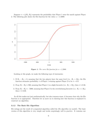
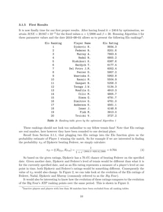
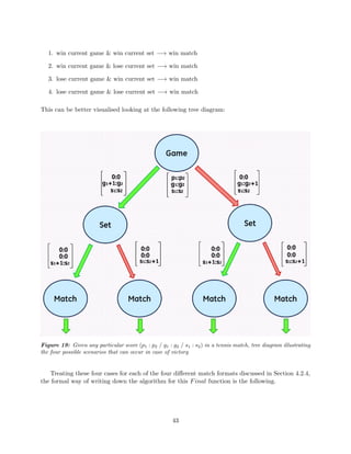
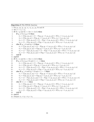
This document is a thesis by Peter Schindler from Imperial College London about improving tennis ranking systems and conducting in-play probability analysis of tennis matches. It uses two main datasets: 1) match result data from 2000-2015 containing winners, scores, rankings, and other information, and 2) point-by-point data from 2014-2015 matches scraped from websites. The thesis develops an alternative Elo rating system to rank players, compares it to the ATP rankings, and analyzes the 2014 Wimbledon final point-by-point to track match probability changes and identify important points.


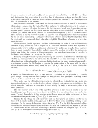
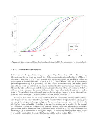
![throughout the entire match. This obviously is not true, and let us show why by giving a simple
demonstration. Let us assume we have a 0.5 prior probability for Player 1 winning a set against
Player 2. Say if Player 1 wins the first set, common sense dictates that his probability of winning
the second set is now more than 0.5 and so we ought to update our prior to something more suitable
like 0.6 for example. Hence the match-win probability with score 2:0 would not be 0.5 × 0.5 but
0.5 × 0.6 instead.
Generalising this idea, the first step would be to define a strictly increasing function w, such
that w : [0, 1] → [0, 1], w(0) = 0, w(1) = 1 and w(π ) > π for π ∈ (0, 1). This function would
have the role of increasing the set-win probability of the winner of the current set by an appropriate
amount. For our previous little example, we would have had w(0.5) = 0.6. Then if we define a
function l to be one that decreases the set-win probability if the current set is lost, then a wise
choice for l would be the inverse of w. In other words, after having won and lost equal amount of
sets, the set-win probability will once again just be the prior: l(w(π)) = π. So in the case of best
of 3 sets, the match win probability would be calculated by summing the probability of winning
2:0 plus the probability of winning 2:1 having lost the first set plus the probability of winning 2:1
having lost the second set:
π = π × w(π ) + (1 − π ) × l(π ) × w(l(π )) + π × (1 − w(π )) × l(w(π )) (6)
Similar computations could be applied to best of 5 set matches. If we manage to find an appropriate
w function, this methodology will allow us to get better match-win probabilities and hence we can
hope for improved error measures.
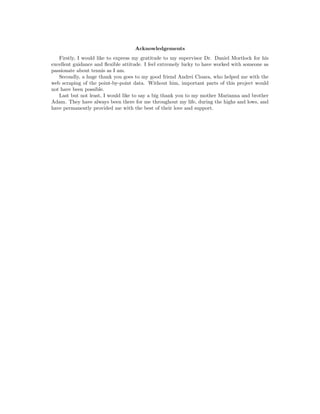
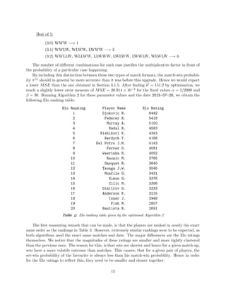
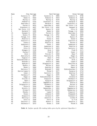
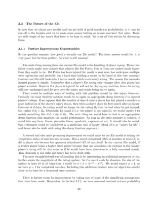
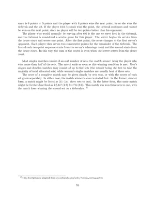
3.3.2 Elo vs. ATP Rankings
The official ATP rankings have been in place since 1973. It allows the ranking of professional tennis
players using a very comprehensible method, presented in detail in division 7.2 of the Appendix.
It is highly important for these rankings to be accurate, because apart from being an indication of
relative strength, it is used to determine which players are allowed to enter which tournaments, as
well as the seedings11 for all tournaments. But how good are these ATP rankings actually? How
good are they in comparison to our Elo rankings?
Let us first look at these rankings from the point-of-view of match prediction. How often does
the higher ranked player win? To give us an idea on how good of a predictor a ranking system is,
a worthy indicator could be the percentage of times the higher ranked player wins. If the higher
ranked player wins 100% of the time, that ranking system would be considered to be perfect; whereas
a ranking system forecasting the higher ranked to win only 50% of the time should be considered
as a baseline, as its prediction power is no better than a coin-flip.
For the current ATP rankings, the higher ranked player wins 65.6% of time. This is a solid value,
far better than the baseline 50%, and hence its usage in the real world is nowhere near catastrophic.
However this value is 66.7% for our Elo rankings from Section 3.2.1 and as high as 67.6% for our
surface specific Elo in Section 3.2.2. These represent respectively a 7% (66.7−65.6
65.6−50 × 100%) and a
13% improvements compared to the ATP rankings. Hence one might rightfully argue that the Elo
ranking systems developed in this thesis is a strong competitor of the current one.
11
For a full explanation on what tennis seedings are, go to the en.wikipedia.org/wiki/Seed(sports) website.
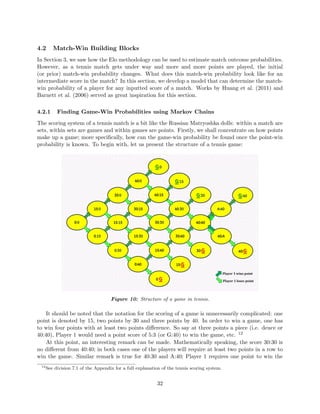
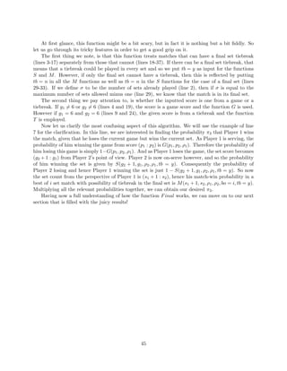
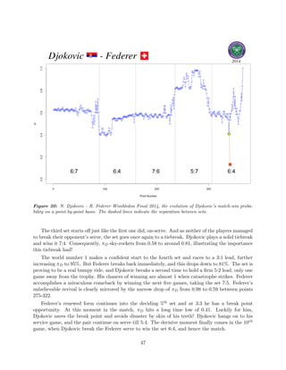
24](https://image.slidesharecdn.com/8aefbcd9-28f8-4607-8461-c883b628cdf0-150928185724-lva1-app6892/85/MASTERS_THESIS_PDF-29-320.jpg)
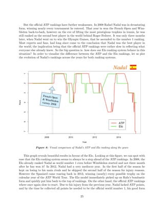
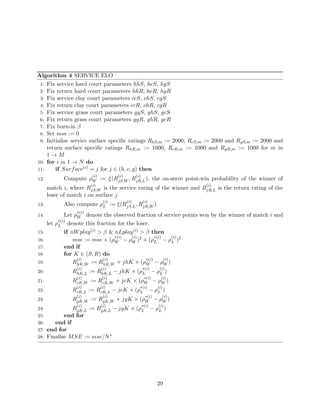
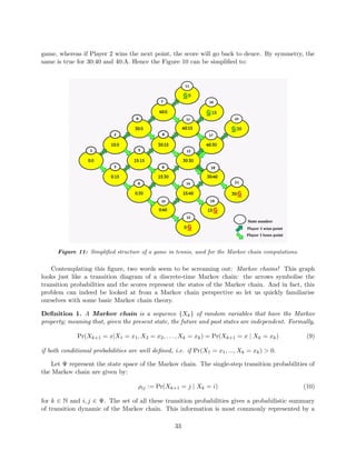
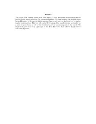
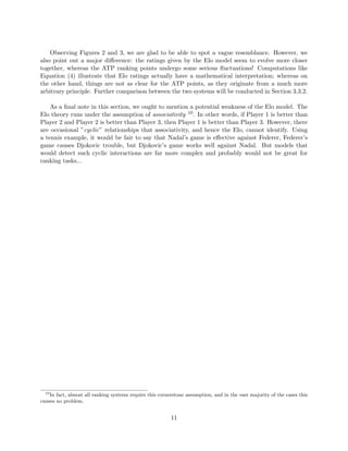
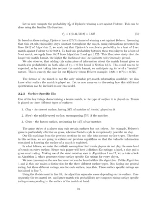
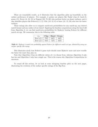
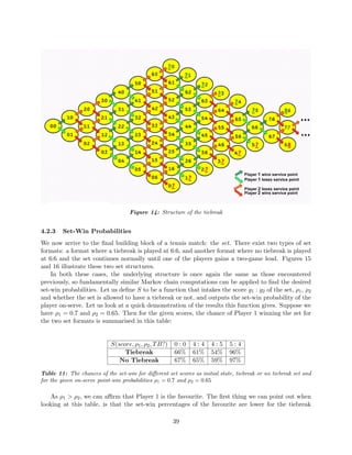
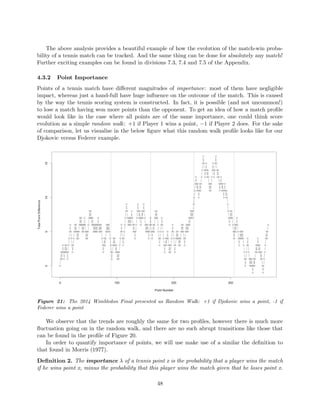
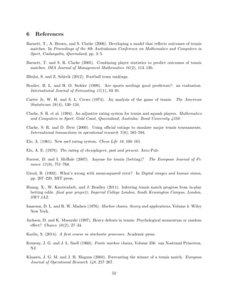
![Basically what this theorem 13 is telling us, is that if we know the initial distribution and the
transition matrix of a Markov chain, the entire dynamics of the chain can be deduced. Let us
demonstrate this using an example. Suppose that two players are at the beginning of a game at 0:0
(State1) and we are given that ρ = 0.5. Hence our initial vector is defined to be the following:
> state <- 1
> u0 <- matrix(0,1,21)
> u0[state] <- 1
> u0
[,1][,2][,3][,4][,5][,6][,7][,8][,9][,10][,11][,12][,13][,14][,15][,16][,17][,18][,19][,20][,21]
1 0 0 0 0 0 0 0 0 0 0 0 0 0 0 0 0 0 0 0 0
Then the first point of the game is played. The chain can either move to State2 with probability
ρ = 0.5 or to State3 with probability 1 − ρ = 0.5. This is illustrated by applying Equation (11) the
above theorem:
> u0 %*% (P %^% 1)
[,1][,2][,3][,4][,5][,6][,7][,8][,9][,10][,11][,12][,13][,14][,15][,16][,17][,18][,19][,20][,21]
0 0.5 0.5 0 0 0 0 0 0 0 0 0 0 0 0 0 0 0 0 0 0
Continuing this process for 2, 3, 4, 5 and 6 points played, the probability distribution evolves
the following way:
> u0 %*% (P %^% 2)
[,1][,2][,3][,4][,5] [,6][,7][,8][,9][,10][,11][,12][,13][,14][,15][,16][,17][,18][,19][,20][,21]
0 0 0 0.25 0.5 0.25 0 0 0 0 0 0 0 0 0 0 0 0 0 0 0
> u0 %*% (P %^% 3)
[,1][,2][,3][,4][,5][,6] [,7] [,8] [,9] [,10][,11][,12][,13][,14][,15][,16][,17][,18][,19][,20][,21]
0 0 0 0 0 0 0.125 0.375 0.375 0.125 0 0 0 0 0 0 0 0 0 0 0
> u0 %*% (P %^% 4)
[,1][,2][,3][,4][,5][,6][,7][,8][,9][,10] [,11][,12] [,13][,14] [,15][,16][,17][,18][,19][,20][,21]
0 0 0 0 0 0 0 0 0 0 0.063 0.25 0.375 0.25 0.063 0 0 0 0 0 0
> u0 %*% (P %^% 5)
[,1][,2][,3][,4][,5][,6][,7][,8][,9][,10][,11][,12][,13][,14][,15] [,16] [,17] [,18] [,19][,20][,21]
0 0 0 0 0 0 0 0 0 0 0.063 0 0 0 0.063 0.125 0.313 0.313 0.125 0 0
> u0 %*% (P %^% 6)
[,1][,2][,3][,4][,5][,6][,7][,8][,9][,10][,11][,12][,13][,14][,15] [,16][,17][,18][,19] [,20] [,21]
0 0 0 0 0 0 0 0 0 0 0.063 0 0.313 0 0.063 0.125 0 0 0.125 0.156 0.156
We notice, that once an amount of probability arrives to an absorbing state, it stays there for-
ever. Remember, our main interest lies in finding the probability gρ that Player 1 wins the game.
This game-win probability is given by the sum of the probabilities of winning the game losing no
points; losing only one point; losing two points, plus the probability that the game goes to 40:40,
but it is still won.
13
The proof of this theorem can be found in Chapter 2.3 of Karlin (2014).
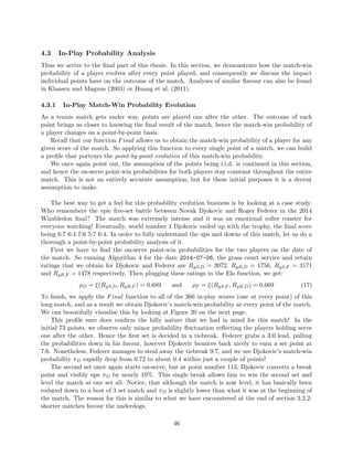
35](https://image.slidesharecdn.com/8aefbcd9-28f8-4607-8461-c883b628cdf0-150928185724-lva1-app6892/85/MASTERS_THESIS_PDF-40-320.jpg)
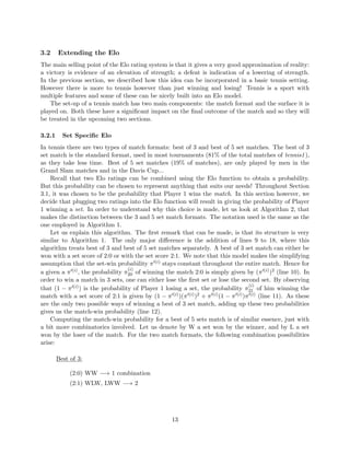
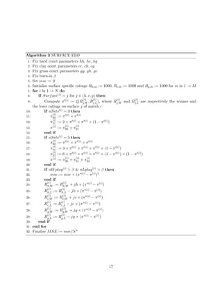
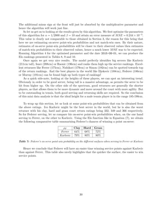
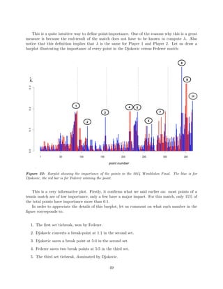
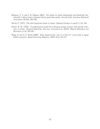
![We can find the expression for D(ρ) going through the following steps:
D(ρ) = Pr(Player 1 wins game with the next 2 points) + Pr(Player 1 wins game after another deuce)+
Pr(Player 1 wins game after 2 deuces) + Pr(Player 1 wins game after 3 deuces) + ...
= ρ2
+ 2ρ2
[ρ(1 − ρ)] + 4ρ2
[ρ(1 − ρ)]2
+ 8ρ2
[ρ(1 − ρ)]3
+ ...
= ρ2
(1 + 2[ρ(1 − ρ)] + [2ρ(1 − ρ)]2
+ [2ρ(1 − ρ)]3
+ ...)
= ρ2
∞
n=0
[2ρ(1 − ρ)]n
=
ρ2
1 − 2ρ(1 − ρ)
using the geometric summation formula
∞
n=0
Xn
=
1
1 − X
if |X| < 1
(13)
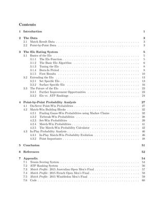
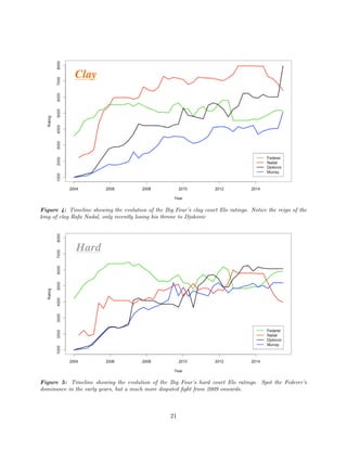
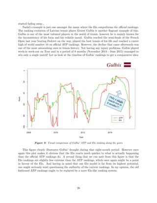
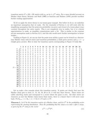
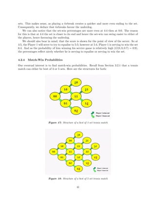
The black curve of Figure 13 plots D(ρ).
Returning to our initial example where we set ρ = 0.5, simple computations give us:
Pr(G|State13) = D(0.5) =
0.52
1 − 2 × 0.5 × (1 − 0.5)
=
0.25
1 − 2 × 0.25
=
0.25
0.5
= 0.5 (14)
And hence:
g0.5 = 0.0625 + 0.125 + 0.15625 + 0.3125 × 0.5 = 0.5 (15)
Concluding this example, if both players have an equal probability of winning a point, then starting
at 0:0, Player 1 has a 50% chance to win the game. This does not seem to be a surprising result
and one might even argue that it is pretty obvious to guess without all the Markov chain business!
However what if ρ = 0.5? What if ρ is something like ρ = 0.64? Applying similar computations as
above, we get the values needed for Formula (12):
g0.64 = Pr(State11) + Pr(State16) + Pr(State20) + Pr(State13) × Pr(G|State13)
= 0.168 + 0.242 + 0.217 + 0.245 × 0.760
= 0.813 (16)
Therefore if a player wins a point 64% of the time, this will result in him winning the game in about
81% of the cases. To picture this, we can look at the blue curve of Figure 13.
Thus far we only looked at game-win probabilities for the initial state being 0:0 and 40:40.
However the same method works perfectly for any other score being the initial state; the only thing
that needs to be changed is the initial distribution vector u(0). Let us define G to be a function that
intakes the point score (p1 : p2) within the game as well as the point-win probability ρ of the player
on-serve, and outputs the game-win probability of that player. As an end for this subsection, let us
take a look at how this function behaves for various point-scores as the initial state:
37](https://image.slidesharecdn.com/8aefbcd9-28f8-4607-8461-c883b628cdf0-150928185724-lva1-app6892/85/MASTERS_THESIS_PDF-42-320.jpg)

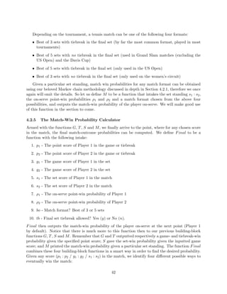
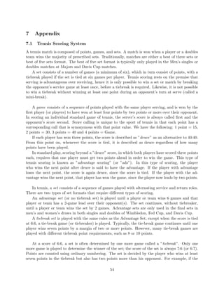
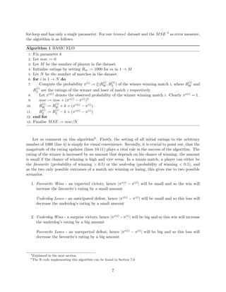
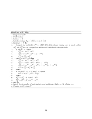
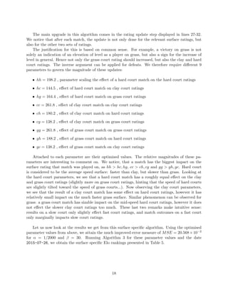
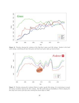
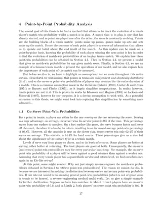
![7.6 Code
#################
### BASIC ELO ###
#################
#set desired date
today <- Sys.Date(); myDate <- as.Date("2015-08-01")
uptil <- max(which(tennis1$Date<=myDate))
daf <- tennis1[1:uptil,]
#fix 1/alpha
bel <- 2000
#fix beta
minMatch <- 0; daf$both <- 0
ix <- which(daf$nplayedW>minMatch & daf$nplayedL>minMatch)
daf$both[ix] <- 1
#the function
ELO <- function(vect)
{
# INITIALIZATION
{
#parameters
k <- vect[1]
#create player IDs
players <- sort(unique(c(daf$Winner,daf$Loser)))
Wid <- match(daf$Winner, players); Lid <- match(daf$Loser, players)
daf$WinnerID <- Wid; daf$LoserID <- Lid
#counting number of matches each player played in total in the dataset
matchCount <- matrix(0,length(players),1)
for(i in 1:length(players)){matchCount[i] <-
length(which(daf$WinnerID==i)) + length(which(daf$LoserID==i))}
#initialising
rating <- rep(1000, length(players))
MSE <- 0
}
# LOOPING
for (i in 1:nrow(daf))
{
#extract ratings
rW <- rating[Wid[i]]; rL <- rating[Lid[i]]
#define prob of winning the MATCH for player 1
mwProb <- 1/(1 + exp(-(rW - rL)/bel))
#define the observed winner of the match
mwObs <- 1
#error measure update step
if (daf$both[i]==1){MSE <- MSE + (mwObs - mwProb)^2}
#rating update step
rating[Wid[i]] <- rW + k * (mwObs - mwProb)
rating[Lid[i]] <- rL - k * (mwObs - mwProb)
60](https://image.slidesharecdn.com/8aefbcd9-28f8-4607-8461-c883b628cdf0-150928185724-lva1-app6892/85/MASTERS_THESIS_PDF-65-320.jpg)
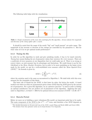
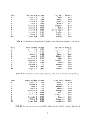
![}
# OUTPUT
div <- length(which(daf$both==1))
MSE/div
}
#####################
### THE OPTIMISER ###
#####################
#set initial parameter value and jump size
para <- c(300)
dim <- length(para)
jump <- c(1)
#required to start the while loop
scoreInit <- ELO(para); scoreNew <- scoreInit - 0.00000000000001
#while loop that runs till there is an improvement in the MSE
while (scoreInit > scoreNew)
{
scoreInit <- scoreNew
scoreOld <- scoreNew
for (i in 1:dim)
{
#first try one parameter value above
scoreTry <- ELO(para+jump*diag(dim)[i,])
if(scoreTry<scoreOld)
{
para <- para+jump*diag(dim)[i,]
scoreNew <- scoreTry
}
else
{
#if not, try one value below
scoreTry <- ELO(para-jump*diag(dim)[i,])
if(scoreTry<scoreOld)
{
para <- para-jump*diag(dim)[i,]
scoreNew <- scoreTry
}
}
scoreOld <- scoreNew
}
}
The picture on the front cover is a Getty Images photo.
61](https://image.slidesharecdn.com/8aefbcd9-28f8-4607-8461-c883b628cdf0-150928185724-lva1-app6892/85/MASTERS_THESIS_PDF-66-320.jpg)


