Esitelma pidetty Saarmaapaivana 2012 syyskuussa

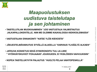
1. 17. lokakuu 2015
0
Maapuolustuksen
uudistuva taistelutapa
ja sen johtaminen
• TAISTELUTILAN MUOKKAAMINEN ”JOS VASTUSTAJA VALMISTAUTUU
JALKAPALLOKENTÄLLE, NIIN ME OLEMME KAUKALOSSA KIEKKOILEMASSA”
• VASTUSTAJAN ENNAKOINTI ”KATSE YLÖS KIEKOSTA”
• JÄRJESTELMÄVAIKUTUS SYVÄLLÄ ALUEELLA ”KARVAUS YLHÄÄLTÄ ALKAEN”
• JATKUVA KOSKETUS SEKÄ SYNKRONOITU TULI JA LIIKE
” HYÖKKÄYSKUVIOT POHJAAVAT JOUKKUEEN, EI YKSILÖIDEN VAHVUUKSIIN”
• NOPEA TAISTELUKYVYN PALAUTUS ”HUOLTO PELAA VAIHTOPENKILLÄ”

2. 17. lokakuu 2015
1
Maavoimien uudistettu
taistelutapa – Mikä muuttuu?
• Tärkein muutos on luopuminen ”jäykähköstä” asemapuolustuksesta.
• Vastustajalle aiheutetaan sellaiset kalusto- ja henkilöstötappiot, että
se ei kykene jatkamaan hyökkäystä suunnitelmansa mukaisesti.
• Huolellisilla valmisteluilla, hajautetulla ryhmityksellä ja väistämällä
vihollisen tulivalmisteluja vähennetään omia tappioita.
• Taistelussa sovelletaan aktiivisesti ja monipuolisesti eri taistelulajeja
sissitoiminnan keinoista puolustukseen, hyökkäykseen ja viivytykseen
ratkaisun saavuttamiseksi.
• Asejärjestelmistä siirrytään taisteluosaston taistelujärjestelmään ja
sen kokonaisvaikutuksen käyttämiseen

3. 17. lokakuu 2015
2
54
14PR Vuokko
27
KUHMO
662
81
759
SUOMUSSALMI
44
27
S
1
2
RAATTEEN TIE
OS Kari
AKTIIVISUUS, LUOVUUS, NOPEA VOIMAN LISÄÄMINEN,
”MAASTOKELPOISUUS”, NOPEUS, VOIMIEN
NOPEA KESKITTÄMINEN, ALOITTEEN TEMPAAMINEN
JOHTI VOITTOIHIN
KUVAN KARTAT NYKY-SUOMEN KARTTOJA!
Uudistettu taistelutapa = avataan
ajattelua omalla taktiikan historialla

4. 17. lokakuu 2015
3
Maavoimien uudistetun
taistelutavan toteutus
Vaatimuksia omille joukoille ja toiminnalle
• Liikkuvuus
• Kyky toimia hajautettuna
• Salaaminen ja harhauttaminen
• Tiedustelu- ja valvonta
• Kyky voiman ajalliseen ja paikalliseen
keskittämiseen
• Kyky operatiiviseen tulenkäyttöön
• Kaukovaikuttaminen
• RSRAKH
• Ilmasta maahan kyky
• Erikoisjoukot
• Yhteisoperaatiot
Kyky vaikuttaa nopeasti viholliseen koko taistelualueella
Haluttuun loppuasetelmaan päästään
aiheuttamalla viholliselle kumulatiivisesti
kasvavat tappiot
UHKALÄHTÖISYYS

5. 17. lokakuu 2015
4
Maavoimien Esikunta
UUDISTETUN TAISTELU PÄÄVÄLINE - TAISTELUOSASTO
JoukkueRyhmä
Konekiväärit
tarkkuuskivääri
pimeäkiikarit
konekiväärit
ITKK
tarkkuuskiväärit
kevyet kertasingot
pimeäkiikarit
lämpötähystimet
TSTJJ
Komppania
kevyet kertasingot
LÄHIPST -ohjukset
kevyet KRH:t
ITKK:t
YKSIKÖN JOJÄ
kevyet kertasingot
PST -ohjukset
raskaat KRH:t
kenttätykit
mini-UAS –lennokkijärjestelmä
TSTOS JOJÄ
Taisteluosasto
EVK
KRHK
HK
PIONK
PSTO
3-4 x JK
RJOHT
TARKAM
RKM (VM)
RKM (PION)
KKAMP
RKM
VARA-
JOHT
KKAMP
TSTPELASTAJA
3 X JÄÄKR
3-4 x JÄÄKJ
KNTOJ
KRHJ
HJ
PS -miinat, kylkipanokset, viuhkapanokset
JOHTO TJR KULJ:t

6. 17. lokakuu 2015
5
Jalkaväkikomppanian
suorituskykytavoite
• Jalkaväkikomppania kykenee hajautuneena
partioittain pimeässä maastossa säilyttämään
tuntuman vastustajaan, iskemään oikea
aikaisesti keskitetyllä tai hajautetulla tavalla ja
ryhmittymään tuntuma säilyttäen uuteen
iskuun.
• Komppanian rungolle on kyettävä liittämään
eri aselajijoukkoja noin 1.5 kertaisesti
perusvahvuuteensa verrattuna ja komppanian
on kyettävä käyttämään muualta tulevaa
tukea joko taisteluosaston tai alueellisen
puolustusjärjestelmän palveluiden kautta.

7. 17. lokakuu 2015
6
MAPU johtamisen suorituskykylisä
• RINNAKKAINEN SUUNNITTELU
• VAST VAIHTOEHTOJEN POISSULKEMINEN
• OPERATIIVINEN YLLÄTYS
• MAALITILANNEKUVA PARANTAA KOSKETUSTA
• KYKY JOHTAA OMIA VASTUSTAJAN RYHMITYKSESSÄ
• HAJAUTETUN TOIMINNAN KOORDINOINTI
• OPTIMOITU VAIKUTUS KUHUNKIN MAALIIN
• JÄRJESTELMÄVAIKUTUKSEN KÄYTTÖ JOUSTAVASTI
• HEIKKOIHIN KOHTIIN KOHDISTUVA VAIKUTUS
• ALUEHUOLLON SUUNNITTELU
• KRIITTISTEN SUORITUSKYKYJEN PALAUTTAMINEN
• VERKOSTO TUKEE TAISTELIJAA

8. 17. lokakuu 2015
7
Uudistusprosessin loppuasetelma
- uudistettu alueellisen puolustuksen taistelutapa
- uudistettu maavoimien joukkorakenne ja modulaariset kokoonpanot
- verkostopuolustus (koko yhteiskunnan voimavarojen hyödyntäminen ja
kansainvälinen yhteistyö)
- vaikuttamislähtöisyys (optimointi, kaukovaikuttaminen, operatiivinen tulenkäyttö)
- joustava johtamisrakenne ilman teknisiä ja toiminnallisia rajapintoja.
Haluttuun loppuasetelmaan päästään aiheuttamalla hyökkääjälle kumulatiiviset tappiot
Ryhmä t
B Joukkue
Komppania
Tukiasema
Tukiasema
Tukiasema
Parikaapeli
Liityntäverkon solmu
14 kpl
3*Jopa
A JoukkueValokaapelit
ja linkit
MATI op-net
verkon
palvelinhotellissa
MATI
Sanomaliikenne on läpi koko maapuolustuksen
TST-johtoverkko ja
MATI TSTJ
MAPU-liityntäverkko ja
MATI 2
ITVJ liityntä- verkko ja
LEIJONA 3
TST-osastolla on itsenäinen johtamiskyky
Ev TFo
Esikunta
0 km 10 km 20 km 30 km 40 km 50 km0 km 10 km 20 km 30 km 40 km 50 km
XX
XX
PVYHT- TULENKÄYTTÖ
XX
OP-TULENKÄYTTÖ
VASTUSTAJA SIDOTAAN
SYVÄÄN TAISTELUUN
ALOITTEELLISEN
PUOLUSTAJAN KANSSA
VASTUSTAJA SIDOTAAN
SYVÄÄN TAISTELUUN
ALOITTEELLISEN
PUOLUSTAJAN KANSSA
KUSTANNUS-
TEHOKKUUS
PAREMPI
TILANNEKUVA

9. 17. lokakuu 2015
8
Kysymyksiä – kommentteja?
• TAISTELUTILAN MUOKKAAMINEN
• VASTUSTAJAN ENNAKOINTI
• JÄRJESTELMÄVAIKUTUS SYVÄLLÄ
ALUEELLA
• JATKUVA KOSKETUS SEKÄ
TULEN JA LIIKKEEN KÄYTTÖ
• NOPEA TAISTELUKYVYN PALAUTUS