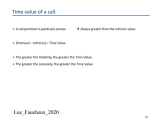
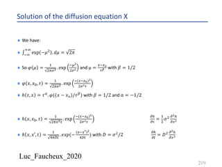
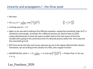
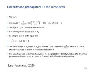
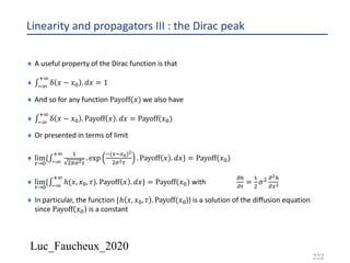
Download as PDF, PPTX


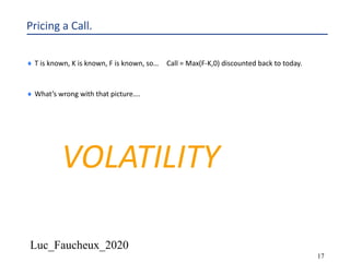


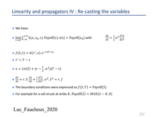
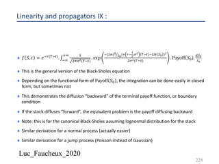
![Luc_Faucheux_2020
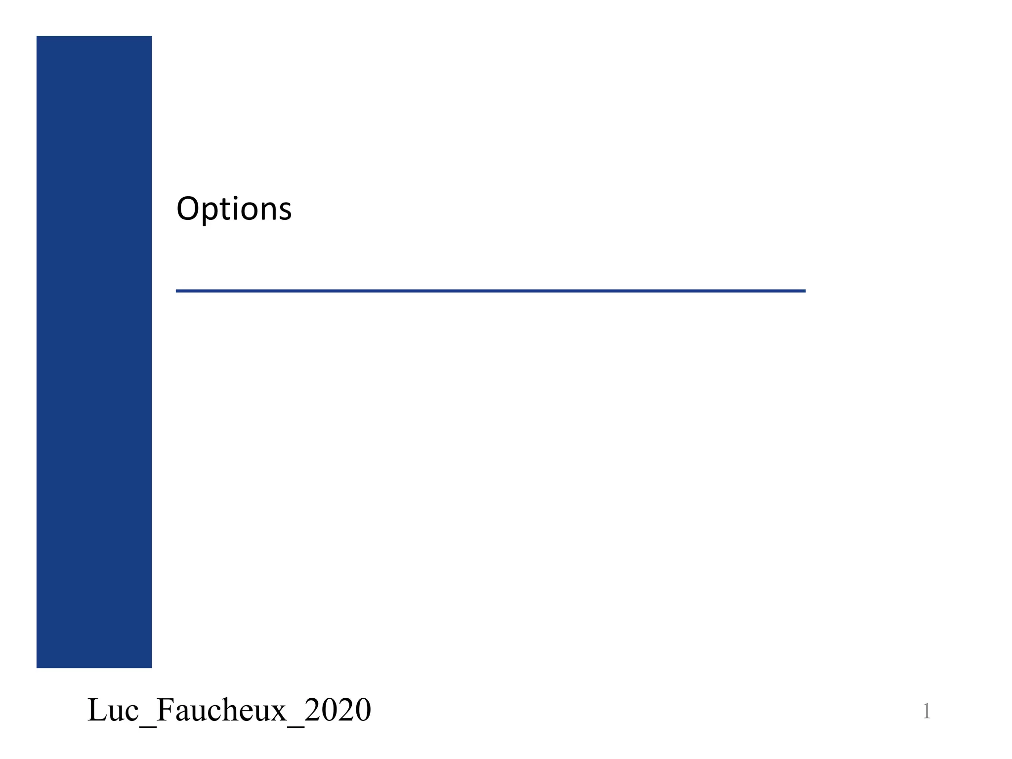
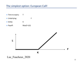
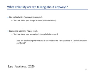
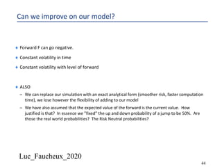
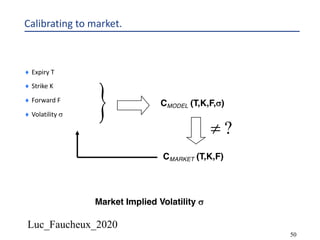
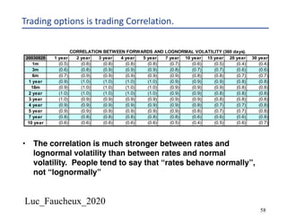
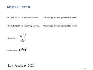
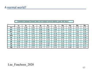
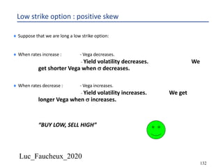
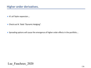
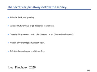
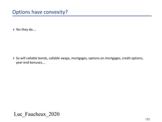
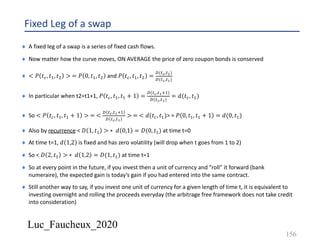
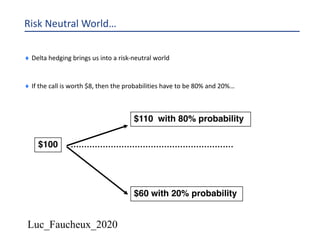
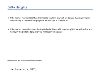
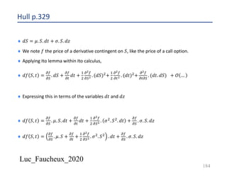
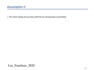
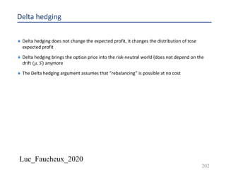
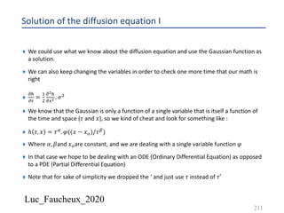
Standard Swap periods
¨ On the fixed side, coupon payment at the end of the period
– Period start date (psj)
– Adjusted period start date (psj_adj)
– Period end date (pej)
– Adjusted period end date (pej_adj)
– Payment date (pmj)
– PV of a period 𝑃𝑉 𝑗 = 𝐷𝐶𝐹 𝑗 . 𝐷 𝑗 . 𝑁 𝑗 . 𝑅 = 𝐷𝐶𝐹 𝑝𝑠𝑗$%#, 𝑝𝑒𝑗_𝑎𝑑𝑗 . 𝐷 𝑝𝑚# . 𝑁 𝑗 . 𝑅
¨ On the float side, floating rate sets at the beginning of the period, and pays at the end (Libor in advance or
standard Libor swap, as opposed to Libor in arrears)
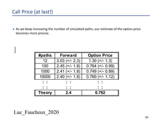
– PV of a period (swaplet) 𝑃𝑉 𝑖 = 𝐷𝐶𝐹 𝑖 . 𝐷 𝑖 . 𝑁 𝑖 . 𝑓 𝑖
– 𝐷𝐶𝐹 𝑖 = 𝐷𝐶𝐹 𝑝𝑠𝑖$%#, 𝑝𝑒𝑖$%# and 𝐷 𝑖 = 𝐷(𝑝𝑚𝑖)
– 𝐷 𝑝𝑒𝑖 = 𝐷 𝑝𝑠𝑖 ∗
&
&'()* +,",+." .0(")
or
– 𝐷𝐶𝐹 𝑝𝑒𝑖, 𝑝𝑠𝑖 . 𝑓 𝑖 = [1 −
( +."
( +,"
]
153](https://image.slidesharecdn.com/lf2020options-200527132347/85/Lf-2020-options-153-320.jpg)
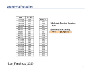
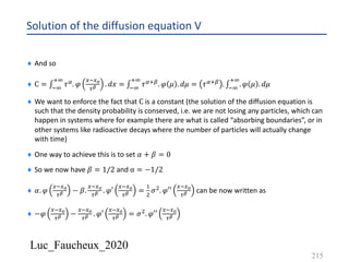
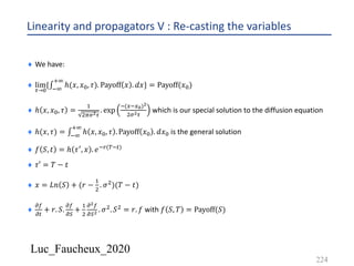
![Luc_Faucheux_2020
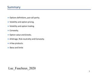
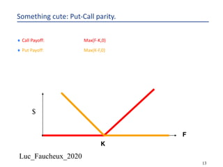
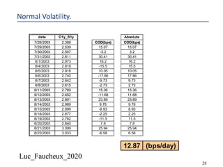
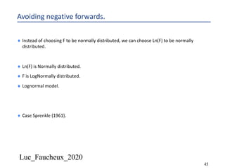
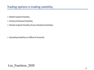
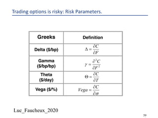
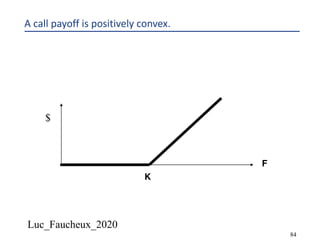
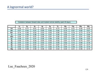
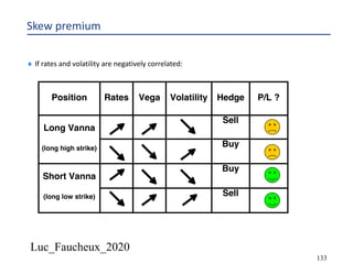
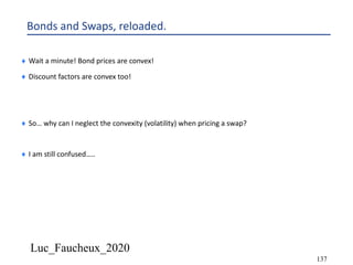
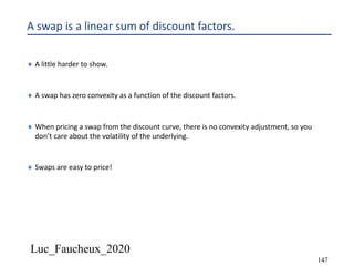
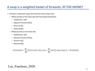
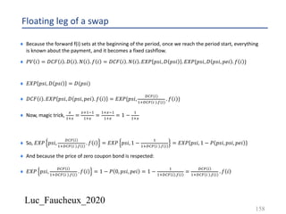
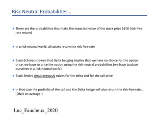
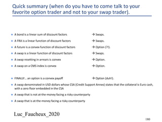
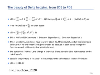
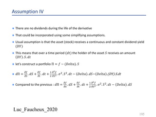
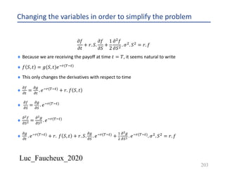
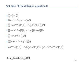
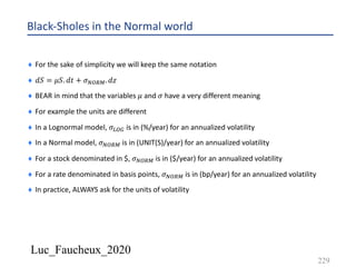
Floating leg of a swap
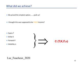
¨ A floating swaplet pays 𝐷𝐶𝐹 𝑖 . 𝑁 𝑖 . 𝑓 𝑖 and its PV is 𝑃𝑉 𝑖 = 𝐷𝐶𝐹 𝑖 . 𝐷 𝑖 . 𝑁 𝑖 . 𝑓 𝑖
¨ Where 𝐷𝐶𝐹 𝑝𝑒𝑖, 𝑝𝑠𝑖 . 𝑓 𝑖 = [1 −
( +."
( +,"
]
¨ We know from the fixed rate leg that < 𝐷 𝑖 >= 𝐷 𝑖 , but what about < 𝐷 𝑖 . 𝑓 𝑖 > ?
¨ Note, to be exact < 𝐷 𝑖 >= 𝐷 𝑖 should really read ∏7#:;7$
𝐸𝑋𝑃{𝑡8, 𝑑(𝑡8, 𝑡8 + 1)}, where
𝐸𝑋𝑃 𝑡8, 𝑑 𝑡8, 𝑡8 + 1 is the expected value of the overnight discount between the time (tc) and (tc+1),
observed up until time tc (because it drops off the curve after tc, and before tc, no matter where you
observe it, its expected value is equal to today’s value)
¨ 𝐸𝑋𝑃 𝑡8, 𝑑 𝑡8, 𝑡8 + 1 = 𝐸𝑋𝑃 𝑡 < 𝑡8, 𝑑 𝑡8, 𝑡8 + 1 = 𝑑(𝑡8 + 1)
¨ Back to < 𝐷 𝑖 . 𝑓 𝑖 > , there is a little trick
157](https://image.slidesharecdn.com/lf2020options-200527132347/85/Lf-2020-options-157-320.jpg)


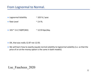
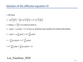
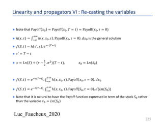
![Luc_Faucheux_2020
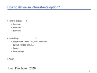
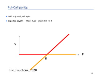
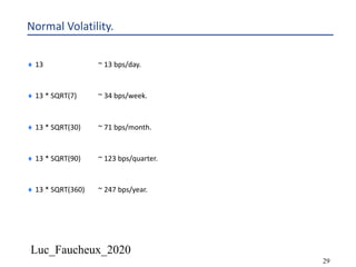
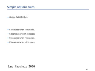
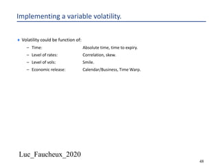
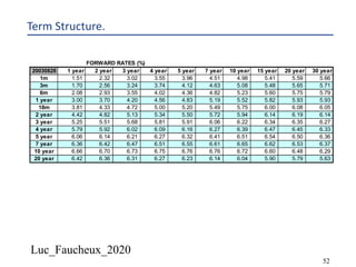
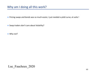
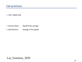
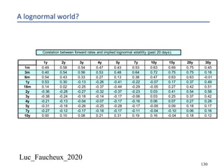
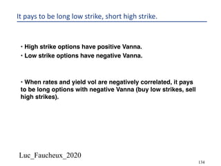
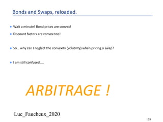
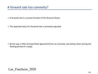
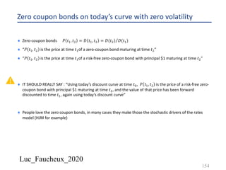
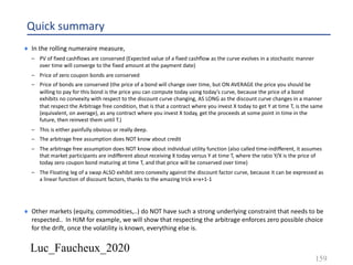
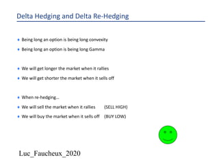
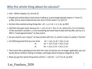
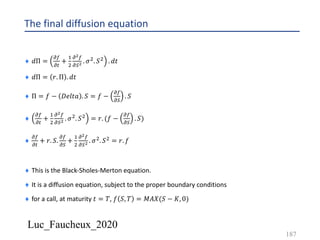
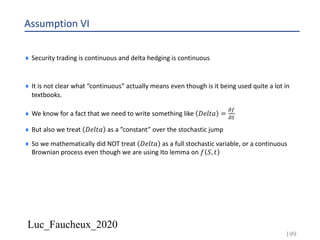
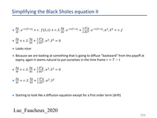
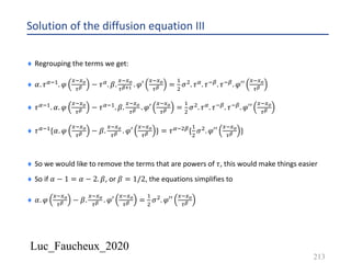
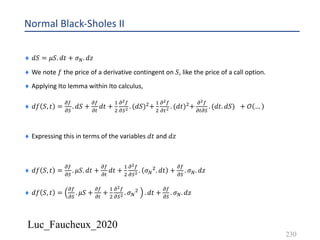
Assumption IV - b
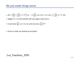
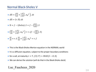
¨ 𝑑Π =
!(
!)
. 𝜇. 𝑆 +
!(
!#
+
&
'
!!(
!)! . 𝜎'. 𝑆' − 𝐷𝑒𝑙𝑡𝑎 . 𝜇. 𝑆 . 𝑑𝑡 + (
!(
!)
. 𝜎. 𝑆 − 𝐷𝑒𝑙𝑡𝑎 . 𝜎. 𝑆). 𝑑𝑧
¨ Becomes
¨ 𝑑Π =
!(
!)
. 𝜇. 𝑆 +
!(
!#
+
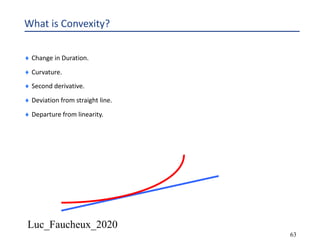
&
'
!!(
!)! . 𝜎'. 𝑆' − 𝐷𝑒𝑙𝑡𝑎 . 𝜇. 𝑆 − 𝐷𝑒𝑙𝑡𝑎 . 𝐷𝑌 . 𝑆 . 𝑑𝑡 + (
!(
!)
. 𝜎. 𝑆 −
𝐷𝑒𝑙𝑡𝑎 . 𝜎. 𝑆). 𝑑𝑧
¨ If we fix 𝐷𝑒𝑙𝑡𝑎 =
!(
!)
, we then obtain
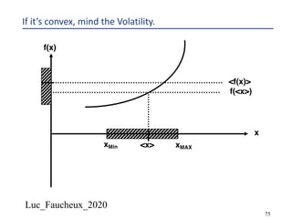
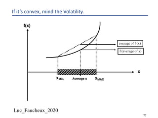
¨ 𝑑Π =.
!(
!#
+
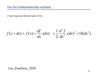
&
'
!!(
!)! . 𝜎'. 𝑆' −
!(
!)
. 𝐷𝑌 . 𝑆 𝑑𝑡 = 𝑟. Π. 𝑑𝑡 = 𝑟(𝑓 −
!(
!#
. 𝑆). 𝑑𝑡
¨
!(
!#
+ 𝑟. 𝑆.
!(
!)
+
&
'
!!(
!)! . 𝜎'. 𝑆' = 𝑟. 𝑓 becomes
!(
!#
+ [𝑟 − 𝐷𝑌 ]. 𝑆.
!(
!)
+
&
'
!!(
!)! . 𝜎'. 𝑆' = 𝑟. 𝑓
196](https://image.slidesharecdn.com/lf2020options-200527132347/85/Lf-2020-options-196-320.jpg)
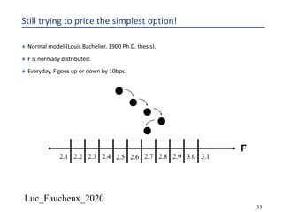
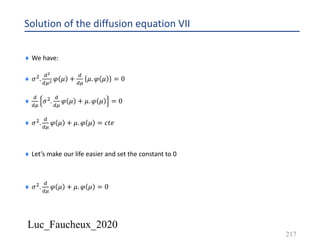
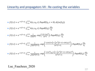
![Luc_Faucheux_2020
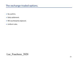
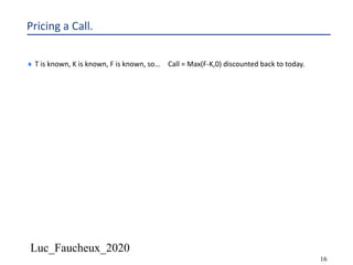
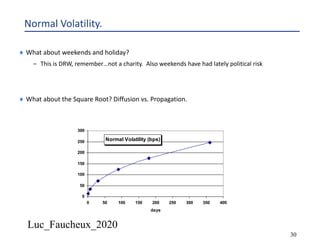
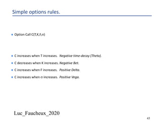
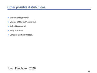
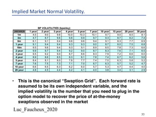
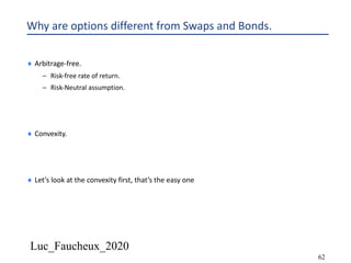
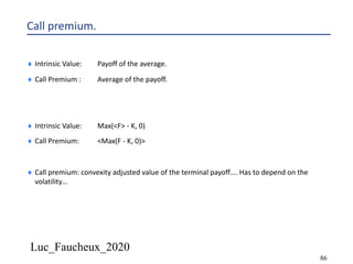
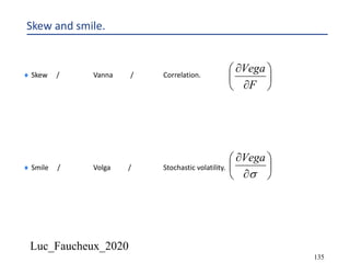
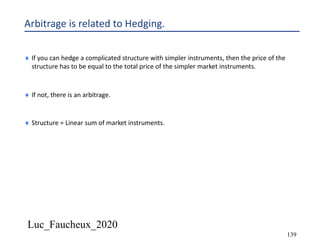
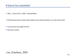
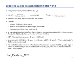
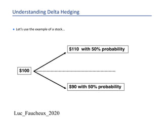
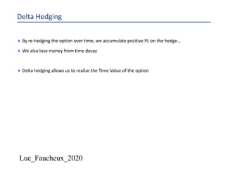
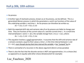
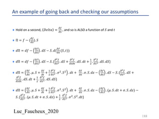
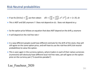
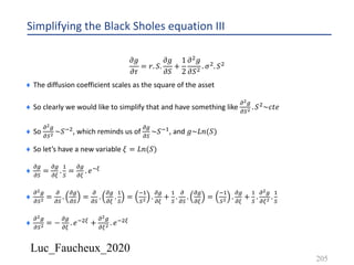
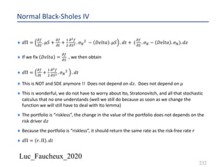
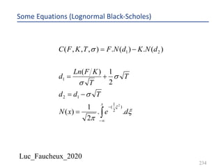
Assumption IV - c
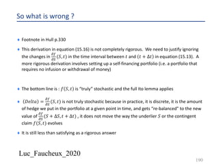
¨ A constant dividend yield is akin to changing the risk-free rate 𝑟 to [𝑟 − 𝐷𝑌 ] but NOT
everywhere, only in the part of the equation that relates to the Delta hedging
¨ So essentially 𝑑𝑆 = 𝜇. 𝑆. 𝑑𝑡 + 𝜎. 𝑆. 𝑑𝑧 becomes 𝑑𝑆 = (𝜇 − 𝐷𝑌 ). 𝑆. 𝑑𝑡 + 𝜎. 𝑆. 𝑑𝑧
¨ Or in the risk neutral valuation that was possible from Delta hedging
¨ 𝑑𝑆 = 𝑟. 𝑆. 𝑑𝑡 + 𝜎. 𝑆. 𝑑𝑧 becomes 𝑑𝑆 = (𝑟 − 𝐷𝑌 ). 𝑆. 𝑑𝑡 + 𝜎. 𝑆. 𝑑𝑧
¨ BUT this is only an adjustment to the stock price process (the portfolio as other riskless
securities will still return the risk-free 𝑟)
197](https://image.slidesharecdn.com/lf2020options-200527132347/85/Lf-2020-options-197-320.jpg)


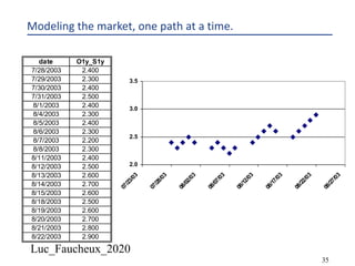
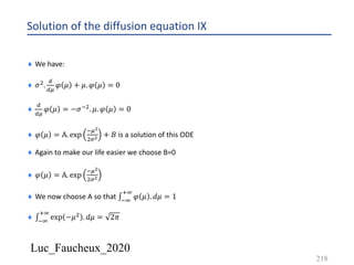
![Luc_Faucheux_2020
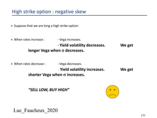
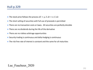
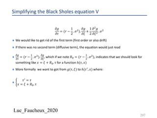
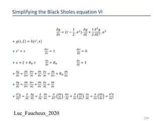
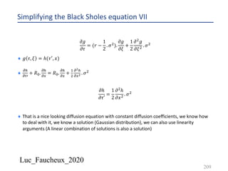
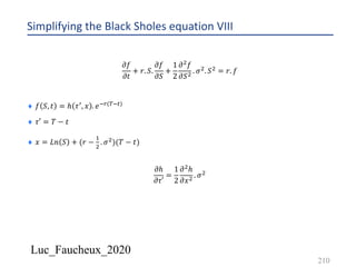
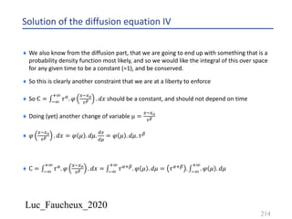
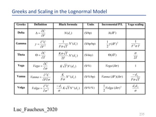
Simplifying the Black Sholes equation IV
¨
!/
!0
= 𝑟. 𝑆.
!/
!)
+
&
'
!!/
!)! . 𝜎'. 𝑆' with 𝜉 = 𝐿𝑛(𝑆)
¨
!/
!)
=
!/
!1
.
&
)
=
!/
!1
. 𝑒*1
¨
!!/
!)! = −
!/
!1
. 𝑒*'1 +
!!/
!1! . 𝑒*'1
¨
!/
!0
= (𝑟 −
&
'
. 𝜎').
!/
!1
+
&
'
!!/
!1! . 𝜎'
¨ Note that this is a little more nicely symmetrical around 0 as if 𝑆 ∈ [0, +∞] we now have
ξ ∈ [−∞, +∞]
¨ Note also that now the coefficients of this equation are NOT function of the variable ξ
¨ We are certainly getting somewhere
206](https://image.slidesharecdn.com/lf2020options-200527132347/85/Lf-2020-options-206-320.jpg)


This document provides an overview of options, including definitions, pricing, and key concepts like put-call parity, volatility, and different types of payoffs. It references various textbooks on quantitative finance and highlights essential topics such as arbitrage, risk analysis, and trading strategies. Additionally, it includes discussions on interest rate options, the importance of volatility, and methods for modeling market behavior.


