Lemna wp 2015-14

Determinants of Bank Lending
Thi Hong Hanh Pham
To cite this version:
Thi Hong Hanh Pham. Determinants of Bank Lending . 2015. <hal-01158241>
HAL Id: hal-01158241
https://hal.archives-ouvertes.fr/hal-01158241
Submitted on 30 May 2015
HAL is a multi-disciplinary open access
archive for the deposit and dissemination of sci-
entific research documents, whether they are pub-
lished or not. The documents may come from
teaching and research institutions in France or
abroad, or from public or private research centers.
L’archive ouverte pluridisciplinaire HAL, est
destinée au dépôt et à la diffusion de documents
scientifiques de niveau recherche, publiés ou non,
émanant des établissements d’enseignement et de
recherche français ou étrangers, des laboratoires
publics ou privés.

Dale Squires
EA 4272
Thi Hong Hanh Pham*
2015/14
(*) LEMNA, Université de Nantes
Laboratoire d’Economie et de Management Nantes-Atlantique
Université de Nantes
Chemin de la Censive du Tertre – BP 52231
44322 Nantes cedex 3 – France
www.univ-nantes.fr/iemn-iae/recherche
Tél. +33 (0)2 40 14 17 17 – Fax +33 (0)2 40 14 17 49
Document
de
Travail
Working
Paper

1
PHAM Thi Hong Hanh1
LEMNA, Institute of Economics and Management, University of Nantes
Chemin de la Censive du Tertre, BP 52231, 44322 Nantes Cedex 3, FRANCE
Phone: +33 (0)2 40 14 17 33 / Fax: +33 (0)2 40 14 16 50
E-mail: thi-hong-hanh.pham@univ-nantes.fr
Abstract: This article aims to empirically investigate the determinants of bank credit by using a large data
set covering 146 countries at different levels of economic development over the period 1990-2013. We find
evidence of the country specific effect of economic growth on bank credit. Our empirical results also suggest
that the health of domestic banking system plays a relevant role in boosting bank lending. By contrast, the
dependence on foreign capital inflows of a country can make its domestic banking sector more vulnerable to
external shock and then to face credit boom-bust cycles.
Keywords: Bank credit; monetary policy; panel analysis
JEL Classification: E51; C23
1 The author gratefully acknowledges financial support from the Chair Finance, Banque Populaire - Caisse
d'Epargne, of the University of Nantes Research Foundation.

2
1. Introduction
As discussed in an orthodox survey (Levine, 2004), financial intermediaries can improve the (i)
acquisition of information on firms, (ii) intensity with which creditors exert corporate control, (iii)
provision of risk-reducing arrangements, (iv) pooling of capital, and (v) ease of making
transactions. This argument favors a well-developed bank-based financial system. Mishkin (2007)
also suggests that a better functioning bank credit system can alleviate the external financing
constraints that impede credit expansion and the expansion of firms and industries.
In addition, several central banks especially consider the role of credit in the conduct of their
monetary policy. For instance, in the European Central Bank (ECB)’s monetary policy strategy
“given the particular importance of bank loans for the financing of euro area firms, developments
in such loans may have important implications for euro area-wide economic activity” (ECB, 2004,
p.20). The Federal Reserve also assigns an important role to credit as “policymakers continue to
use monetary and credit data as a source of information about the state of the economy”
(Bernanke, 2006, p.2). Moreover, Fernandez-Villaverde et al., 2013 argue that utilizing domestic
credit instead of external financing allows a country to ease the pressure coming from the
exchange rate risk on domestic firms.
On the other hand, as discussed in several studies (e.g. Mendoza and Terrones, 2008; Obstfeld and
Rogoff, 2010), a rapid growth of domestic credit supply could play a significant role in predicting
subsequent financial or economic crises, while a deep decline in domestic credit can result in a
recession in economic activity and financial instability. According to Mishkin (2010), the recent
global recession of 2007 also reflected one type of asset price bubble, which can be considered as a
“credit-driven bubble”.
Due to the crucial role of credit in economic activity of a country, there is a growing empirical
literature examining the determinants of domestic credit, which may be demand-side or supply-
side factors. Some studies consider both kinds of factors in the same model, while others try to
distinguish them into two separate models. The determinants of credit supply have been also
studied in the case of advanced, emergent as well as developing countries. Employing a
cointegrating VAR for 16 industrialized countries, Hoffman (2001) finds evidence of a significant
positive relation between domestic credit, real GDP and inflation, but a negative correlation
between credit and real interest rates. Similarly, Calza et al. (2001), using VECM for a sample of
European countries, show that in the long-run domestic credit is related positively to real GDP
growth but negatively to short term and long term real interest rates. Focusing in a large panel of
non-transition developing and industrialized countries Cotarelli et al. (2005) conclude that banking
lending is positively related to GDP per capita, financial liberalization and transparency in

3
accounting standards but negatively depends on the public debt ratio. Differing from the above
cited works, Aisen and Franken (2010) estimate the main determinants of bank credit growth
during the 2008 financial crisis for a sample of over 80 countries. They find that larger bank credit
booms prior to the crisis and lower GDP growth of trading partners are the most important
determinants of the post-crisis bank credit slowdown. On the other hand, structural variables such
as financial depth and integration level are also relevant. Guo and Stepanyan (2011) examine the
changes in bank credit across a wide sample of 38 emerging economies during the last decade.
Their main finding is that domestic and foreign funding contributes positively and symmetrically
to credit growth. In another recent study of 24 emerging countries, Gozgor (2013) argues that the
essential determinants of domestic credit are loose monetary policy in the domestic market,
differences between domestic and global lending rates, and trade openness. On the other hand,
external balance and perceptions of global tail risk negatively affect domestic credit levels.
Even though assessing the determinants of bank credit has been an interesting and growing
subject in the empirical literature, the determinants of credit growth appear to be complex
(Elekdag and Han, 2012). For this reason, we try to revisit and reexamine the possible
determinants of domestic credit, which have been questioned in the literature. Domestic credit
studied in this paper refers to the credit provided by the banking sector to non-financial private
sector. Our study seeks to contribute to the related literature in several ways. First, following the
existing literature, we will introduce all potential demand-side and supply-side factors in the
estimated equation. In addition, we try to empirically model domestic credit level through two
theoretical approaches, notably bank balance sheet and bank capital requirements. Second, the
global financial crisis of 2007–2009 experienced the need for banking systems to be more liquid,
more transparent, less leveraged and less prone to take on excessive risk. Since the recent financial
crisis, banking system has been demanded to build larger buffers of high-quality capital and to
reduce the riskiness of their portfolios. In this context, we aim to resolve the question of how
banking system has adjusted its credit supply to higher capital requirements. Third, we extend our
empirical analysis for a wide sample covering 146 countries at different levels of economic and
financial development during the period of 1990-2013.
The reminder of this paper is organized as follows. Section 2 tries to formulize an empirical
equation of domestic credit supply basing on the different theoretical approaches. Section 3 gives a
descriptive analysis of the variables and the instruments used in the estimation. Section 4
summarizes the data and empirical methodology. Section 5 explains and discusses the empirical
results. The concluding remarks and policy implications are in Section 6.

4
2. Empirical equation
The starting point is a primitive type of bank balance sheet in which the bank has no physical
capital on its assets and no equity on its liabilities. This simple balance sheet is described as
follows:
Assets Liabilities
C: Credits
R: Reserves
D: Deposits
The balance sheet can be represented as follows:
+ = (1)
From the above balance sheet and in developing a framework for the analysis of the banking firm,
Baltensperger (1980) sets the objective function of the bank as a profit function:
= − − − − (2)
Where rC is the interest rate of bank credit, rD is the interest paid on deposits, l is cost of illiquidity,
s is cost due to default, and c is the real resource cost.
From Function (2), we can also generalize the function of credit supply as follows:
= ; ; ; ; ; ; (3)
Now, we consider another type of bank balance sheet in which the bank has credits, reserves and
treasury bills on its assets, and deposits and capital requirements on its liabilities. This balance
sheet is written as follows:
Assets Liabilities
C: Credits
R: Reserves
T: Treasury Bills (free-risk assets)
D: Deposits
K: Capital requirements
In this case, the equation of balance sheet of a bank is presented as follows:
+ + = + = + − − (4)
Basing on this bank balance sheet approach, the determinants of bank credits supply are bank
reserves, treasury bills, bank deposits and capital requirement. In general, credit supply positively
depends on the credit rate of return. This positive relation is, nevertheless, influenced not only by
other costs stemming from the bank’s decision of credit supply but also by other components of
balance sheet such as capital requirements and so on. We now study the most important
determinants to show how they are handled in the model of credit supply.
Analysis of rates of return
A bank may allocate its resources either in credits or in government securities. The rates of return
of a bank include:

5
- Return in credits supply: −
- Return in T-bill investment: − under the condition > >
Considering that is the bank resource allocation in credits and is the bank resource allocation
in T-bills with 0 < + < 1, the function of bank rates of return is given as follows:
= − + − = + − + (5)
The credit supply C is expected to be positively related to its rate of return − , and
negatively to ′, which is the cost of controlling default risk. We assume that these relations are
linear and given as follows:
= ∑ ! − !
"
!# + ∑ ′!
"
!# + $ (6)
where $ is the vector containing other factors determining bank credit supply.
Analysis of capital requirements
The capital requirement ratio (CR) expresses the own funds K of a bank as a proportion of risk
weighted assets and off-balance sheet items.
=
%&'( %)* +,*-. /
0!.1 )2!34&2- '..2&.5"%&!%*'( 6!.1 )2!34&2- 7..2&.
≥ 9 (7)
where the risk weighted assets are the credit risk assets, and the notional risk weighted assets are
the operational risk and market risk (RN). The capital requirement ratio can be rewritten as follows:
=
/
): 5); 50<
≥ 9 (8)
Where w1 is the weight for risky credits and and w2 = 0 is the weight for government securities. It
is assumed that:
=
0 ≤ ? ≤
? @'A = B C C DEFDG DGBF HD IJD B KL DGBF
According to Formula (8), there is a minimum value b required for a bank Basel index, which is the
ratio between capital and risk weighted assets. Moreover, the coefficient w1 defined in regulation
and known by the bank. Following Furfine (2001), we assume that the own capital of a bank
approximates the minimum level stated by the requirement faces increasing costs. That means:
= 9 ↔ =
/
N):
−
0<
):
(9)
Equation (8) means that credit supply positively relates to the own capital of a bank. On the other
hand, it confirms a negative relationship between bank credits, operational and market risks and
the Basel index. From Equations 2-6-9, we obtain the following reduced empirical form of bank
credit supply:
= ∑ ! − !
"
!# + ∑ ′!
"
!# +
/
N):
−
0<
):
− + + + $ (9)

6
3. Data and variables description
This paper empirically examines the determinants of domestic credit levels across a wide range of
countries at different levels of economic and financial development as long as data are available
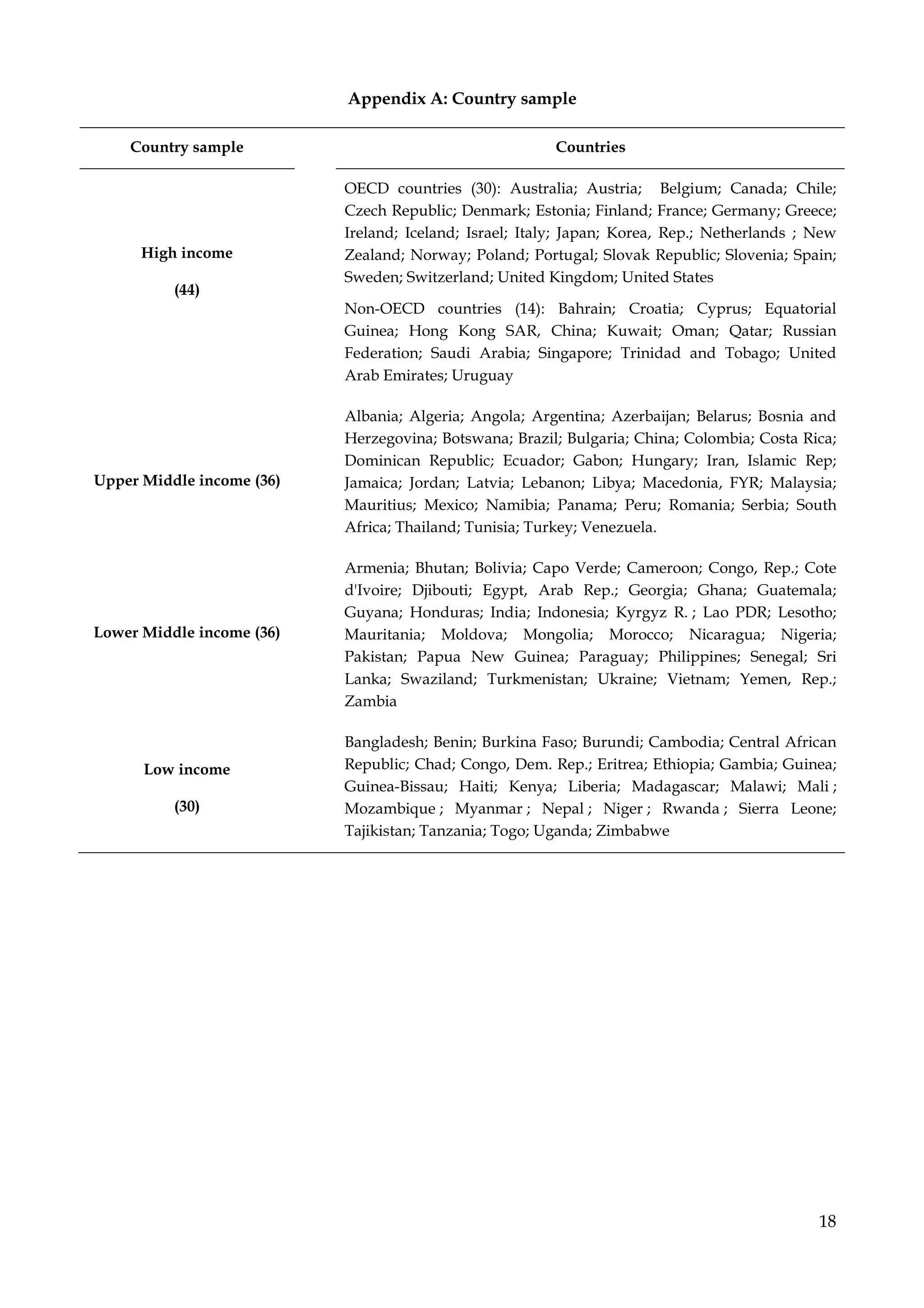
(for the list of countries see Appendix A). We exclude the transition economies and small economies
with a population of less than 500 000 in 2000 from our analysis. The information on the transition
economies and population size are from the World Bank Global Development Network Database
(GDN) and the WDI, respectively. In addition, in order to avoid the potential problem of
heterogeneity in cross-country economic development level, there are five data samples on which
the estimation is based: (i) the whole sample; (ii) high-income sample (HI); (iii) low-income sample
(LI); (iv) lower middle-income sample (LMI); and (v) upper middle-income sample (UMI). Our
analysis employs annual data series from 1990 to 2013, which are collected from many
international data sources: International Financial Statistics (IFS); Global Financial Development
(GFD); Global Financial Development (GFD); and World Development Indicators (WDI). Due to
data unavailability particularly in the case of developing countries, we miss data for some
countries either at the start of the sample or at the end of sample. For this reason, our panel is not
balanced.
With respect to the research objective, the dependent variable is the ratio of domestic credit
provided by banking sector to private sector to GDP. The choice of explanatory variables is based
on either the above reduced form of credit supply or the concerned literature. We explain and
discuss the choice of independent variables as follows.
Internal demand factors
Following Equation 10, we first introduce the following independent variables in our estimation:
- Deposit: This variable is weighted by the share of total domestic deposit to GDP. This
variable allows us to control for the important role of domestic deposits as a funding
source.
- Real interest rate: This variable is measured by the lending interest rate adjusted for inflation
as measured by the GDP deflator.
- Banking management / operation costs: This variable is weighted by total costs as a share of
total income.
- Capital requirement: The ratio of capital requirement is initially provided by Barth et al.
(2001). However, this data is only available for 2000, 2003, 2007 and 2013. For this reason,
our analysis will use two alternative indicators. The first one is the share of bank regulatory
capital to risk-weighted assets. The second one is the share of bank capital to bank assets

7
instead of the ratio of capital requirement. In fact, the evolution of this indicator can
partially reflect the change in capital requirement ratio.
- Systemic banking crisis: We control for the impacts of systemic banking crisis on credit
supply by introducing a dummy variable, which takes the value of 1 during the period of
banking crisis and the value of 0 in other periods.
Second, we introduce other variables used in the literature to capture the impacts of internal
demand factors on credit supply as follows:
- Real GDP per capital in U.S. dollars: This variable is a benchmark measure of the economy
health and reflects the demand for credit (Frankel and Romer, 1999). We expect that higher
domestic income corresponds to stronger domestic demand and higher domestic credit
(Takats, 2010).
- Inflation rate: We introduce the inflation rate based on consumer price indices (2005 = 100)
in the estimation as a control variable to verify the hypothesis of whether there is a
connection between bank credit growth and price stability.
- Domestic money supply: This variable is defined as broad money M3 as a percentage of GDP,
which is considered as a proxy for the overall monetary policy stance. As discussed in a
seminal work, by using IS-LM framework Bernanke and Blinder (1988) analytically show
that monetary policy could have a direct impact on bank lending: lower money supply
leads to less domestic credit growth.
External supply factors
Together with internal demand factors, we also introduce in our estimation a broad set of external
supply factors.
- Nominal exchange rate: As discussed in Borio et al. (2011), a fall in the value of nominal
exchange rate of a country expresses an appreciation of the domestic currency and thus
results in an increase in domestic credit.
- Foreign capital flows: This variable is measured by the share of net foreign direct investment
and portfolio investment to GDP. Increasing private capital flows is expected to increase
the volume of domestic credit (Lane and McQuade, 2013).
- Financial integration level: To capture the level of financial integration, we use the Chinn and
Ito (2006) index of capital account openness (KAOPEN). The tested hypothesis is that
higher financial integration level leads to higher inward capital flows, which in turn
facilitate a country’s financing.
- Trade openness level: this indicator is measured by exports plus imports over GDP. In fact,
higher trade openness can relate to higher bank lending but also makes a country more

8
vulnerable to international shocks such as a dramatic collapse in global trade during the
period 2008-2009.
Global factors
This study also aims at investigating the possible impacts of some global factors on bank credit
supply by introducing in the estimation several explanatory variables as follows:
- The change in U.S. money supply: This variable is measured by the variations of the share of
broad money to GDP and considered as a benchmark indicator of global liquidity variation.
- The change in U.S. Federal funds rate: This variable is used as another proxy for global
liquidity variation. According to Csonto and Ivaschenko (2013), as lower Fed funds rate is
assumed to be associated with higher liquidity, it is expected to have a positive impact on
lending rate and thus to increase lending rates.
- The difference between the domestic lending rate and the US (global) lending rate: The question of
interest is whether the domestic banks can borrow from abroad at lower global interest and
lend at higher domestic interest rates.
- External debt: this variable is measured by the share of total external debt stocks to gross
national income. An expected negative relationship between external debt and bank
lending indicates that a country, with higher international liabilities, is more vulnerable to
international shocks, which in turn limit access to new funding (Aisen and Franken, 2010).
- Systemic banking crisis: to control for the impact of any systemic banking crisis on domestic
credit levels, we use a dummy variable that takes the value of 1 during the financial crisis
period and of 0 in others periods.
Characteristics of the domestic banking system
Following Aisen and Fraken (2010), we assume that bank credit supply is also influenced by the
characteristics of domestic banking system, which are captured by a set of following indicators:
- Bank return on equity (ROE) and bank return on assets (ROA): These two indicators reflect the
benefit of a bank. According to Aisen and Fraken (2010), a bank with sound profitability
will most likely have great access to financing, but it could also indicate that banks have
taken riskier positions.
- Bank concentration: This indicator is constructed by Beck et al. (2000) and defined as total
assets of the three largest banks as a percentage of total assets of the banking system.
- Initial development level of banking system: to capture the impacts of initial level of banking
system development, we simply use the ratio between the banking credit to private sector
and GDP in 1989.

9
- Bank non-performing loans to total gross loans: This variable is to measure the soundness of
banking system, which can strongly influence the growth of domestic credit.
The data sources of all key variables as well as their definition and units of measurement are
summarized in Appendix B.
4. Empirical methodology
The present paper aims to explain the dynamics of bank credit supply across countries through an
analysis of its potential determinants. Given this aim, we endeavor to make maximum use of both
time and cross-country dimensions of available annual data sets. According to Baltagi (2005), using
annual data for estimation purposes necessitates making an allowance for the possibility that the
annual observations on independent variable may not represent long-run equilibrium values in
any given year because of slow adjustment in explanatory variables. To allow for the possibility of
partial adjustment, we determine a dynamic log-linear equation for domestic credit which includes
its lagged dependent variable. Our empirical model is given as follows:
O!& = PQ + P O!&R + P ST !&R + PUOV !&R + PWX Y!&R + PZ Y[!&R + & + $!& (11)
where CREit is the share of bank credit to private sectors in GDP of country i in year t, INTit
represents different internal demand factors, EXTit represents a broad set of external supply
factors, GLOit indicates different global financial market conditions, DOMit represents the
characteristics of domestic banking system, $!& is a disturbance term assumed to satify the Gauss-
Markov conditions, and & is a trend term accounting for a shift of the intercept over time.
However, several econometric problems may arise from Equation 11.
- The independent variables are assumed to be endogenous. This is because causality may
run in both directions – from independent variables to dependent variable and also these
regressors may be correlated with the error term.
- Time-invariant individual characteristics (fixed effects) can be correlated with the
explanatory variables.
- Introducing the lagged dependent variable gives rise to the autocorrelation between the
regressors and the error term since lagged independent variable depends on the country
specific effect. Due to this correlation, the estimation of Equation 11 suffers from the Nickell
(1981) bias.
In this case, a transformation like first-differencing is again required to eliminate the individual
effects from the transformed equations in order to obtain valid moment conditions. However,
differencing introduces a simultaneous problem because lagged endogenous variables will be

10
correlated with the new differenced error term. In addition, heteroscedasticity is expected to be
present because, in the panel data, heterogeneous errors might exist with different panel members.
To resolve these problems, the GMM method developed by Arellano and Bond (1991) seems to
produce more efficient and consistent estimators compared with other procedures. The GMM
method also eliminates any endogeneity that may be due to the correlation of the country specific
effects and the right hand side regressors. This technique treats all the variables other than the
lagged dependent variable by assuming that they are uncorrelated with the error term ε^_.
According to Baltagi (2005), in this case, we should lag all the right hand side regressors by one
period, which makes this assumption more innocuous and is sufficient to prevent any bias in the
estimated coefficients due to simultaneous common shocks to credit supply and the explanatory
variables. If we first difference Equation 11, we get:
∆ O!& = P ∆ O!&R + P ∆ST !&R + PU∆OV !&R + PW∆X Y!&R + PZ∆ Y[!&R + ∆$!& (12)
Equation 12 has removed the group effects and time trend. Arellano and Bond (1991) also develop
the serial correlation test, in which the null hypothesis assumes no serial correlation in error term.
The authors introduce the serial correlation test, often labelled “m1” for first-order and “m2” for
second-order serial correlation. We expect to find first-order serial correlation in the first
differenced residuals. The key problem arises if there is second or higher order serial correlation,
as this would suggest that some of the moment conditions are invalid.
Before estimating the regression of interest, we report the means and standard-errors of dependent
and independent key variables in Table 1. In addition, Table 1 provides the correlation coefficients
between bank credit and all covariates. It can be seen that bank credit variable displays
considerable variation both between and within countries, justifying the use of panel estimation
techniques. As shown in Table 1, most of correlation coefficient are significant. This result aids the
modelling and helps to confirm the choice of dependent variables. However, the values of
correlation coefficient are diverse, ranging from negative to positive, from small to important. For
instance, we find a negative and significant value of correlation coefficient between bank credit
and bank operation costs, while that between bank credit and bank deposit is significantly
positive. Looking at the external supply factors, bank credit is much less correlated to capital
inflows than trade openness. The results on correlation coefficients show that the magnitudes, the
statistical significance even the sign of correlation coefficient have been more or less altered. Thus,
we should not be surprised to see different empirical results for different data samples.

11
5. Empirical analysis
This section reports the results of GMM estimator and robustness tests. It also outlines the results’
implications for the considered theoretical hypotheses. On the other hand, the continuous and
consistent financial data, in particular the data on capital requirement and characteristics of
domestic banking system, are lacking. Therefore, to make maximum use of both time and cross-
country dimensions of available annual data sets, we estimate four following alternative models:
- Model 1 includes all potential explanatory variables.
- Model 2 excludes bank operation costs and capital requirement.
- Model 3 excludes the characteristics of domestic banking system.
- Model 4 excludes bank operation costs, capital requirement, and also the characteristics of
domestic banking system.
<Insert Table 2>
Table 2 reports the GMM results in two parts. The upper show the estimated coefficients and their
robust standard errors for each model of interest. The lower presents the serial correlation test.
According to the results, the first order serial correlations (m1) are expected because of first
differencing, and the p-values obtained suggest no significant second order serial correlation (m2).
Thus, we should reject the null hypothesis of the absence of first order serial correlation and not
reject the absence of second order serial correlation. This result implies that our estimated models
satisfy the required orthogonal conditions.2
Role of internal demand factors. Going straight to the hypothesis of interest, we note that the
estimated coefficients of bank deposit enter in all models with a negative but statistically
insignificant value. This means that there is no direct link between deposits and loans. In other
words, if private sectors do not wish to borrow, no amount of money supply will encourage them
to do so. This result does not support the classical loanable funds theory, according to which bank
loans depend on pre-existent savings. By contrast, bank credit seems to positively depend on
lending interest rate, when all estimated coefficients of this variable are positive and statistically
significant. This is a quite important phenomenon implying that high lending rate may not
necessarily translate into poor lending performance or lower proportion of commercial banks’
funds available for lending respectively. Another potential determinant of bank credit is the share
of operation costs in total income. In all regressions, the coefficients have the expected negative
signs but statistically insignificant. Regarding the capital requirements, they all come out with the
2
Together with the serial correlation test, another key test of the GMM estimator is the Sargan test to assess the model
specification and over-identifying restrictions, whether the instruments, as a group, appear exogenous. This test is also
known in the GMM context as Hansen’s J test. However in this paper, the Sargan test’s results are not reported since it is
not possible to estimate the Sargan statistic with robust to heteroskedasticity standard errors.

12
expected negative signs and statistically significant. For instance, an increase in regulatory capital
can reduce the supply of loans, meaning that there is a trade-off between solvency and loan
supply. On the other hand, higher level of capital corresponds to more important credit supply.
We now turn our attention to other explanatory variables concerning economic activity. First, we
find that economic growth captured by GDP per capita does not play any significant role in
explaining bank lending. This result is not consistent with the hypothesis of a pro-cyclical
relationship between economic growth and bank lending. For instance, Dell’Ariccia and Marquez
(2006) suggest that bank credit expansions tend to be pro-cyclical, meaning that high economic
growth tends to induce a high level bank credit supply. Precisely, during the period of economic
boom, banks relax their criteria of selection and lend to both efficient and less efficient projects,
while during the period of economic recession, bank credit dries up due to a high level of
nonperforming loans and default risk. Second, we reveal an expected negative but insignificant
relationship between inflation and bank lending. The negative impact of inflation on bank credit
has been widely explained by the existing literature. For example, according to Huybens and
Smith (1998, 1999), high inflation is detrimental to the development of the financial system when it
limits the amount of external financing available to borrowers. Furthermore, Boyd et al. (2001)
suggest that in high inflation environments, financial intermediaries are less willing to engage in
long-run financial projects. Rousseau and Wachtel (2002, p.780) also argue that “high inflation will
discourage any long term financial contracting and financial intermediaries will tend to maintain
very liquid portfolios. In this inflationary environment intermediaries will be less eager to provide
long-term financing for capital formation and growth.” Third, we consider the liquidity effects on
bank credit growth by using the monetary supply. In contrary to the insignificant effect of
economic growth and inflation, the coefficients of monetary supply are highly statistically
significant and have the expected positive sign. This means that monetary policy could have a
direct impact on bank lending, which is so-called “ bank credit channel” of monetary policy: an
increase in liquidity allow banks to expand their supply of loans and thus making credit more
available to bank-dependent borrowers (e.g. Bernanke and Blinder, 1992; Kashyap and Stein, 2000).
Role of external supply factors. First, we consider the exchange rate as one of relevant external
supply factors influencing bank lending. As reported in Table 2, the estimated coefficients
associated to the exchange rate variable are negative and strongly significant. This result supports
the negative impact of exchange rate on credit supply, which can be explained in two ways. On the
one hand, an increased value of domestic currency of a country can reduce its exports, which in
turn negatively influences domestic bank credit. On the other hand, the devaluation of domestic
currency of a country may also reflect a risky economic environment that worsens bank credit

13
supply. Second, we find that economic integration differently influences bank lending. The
estimated coefficients of FDI flows enter in all models with the expected positive sign but
statistically insignificant value. Accordingly, domestic bank credit does not depends on inward
FDI. In other words, we can consider foreign investment as a funding source of domestic economic
activities rather than a source of bank lending. Similarly, we do not find evidence that higher trade
openness can contribute to bank credit. By contrast, when we control for the characteristics of
domestic banking systems (Model 1-2), the KAOPEN index has negative and significant
coefficients. This is because higher financial integration facilitates a country’s financing, but it also
makes it more vulnerable to international shocks. High vulnerability of banking systems can, in
turn, reduce their credit supply.
Role of domestic banking system’s characteristics. As mentioned above, the present paper also
tends to revisit the impact of the characteristics of domestic banking system on bank credit growth.
First, we find no evidence of an interaction between ROE/ROA and bank credit supply. This result
does not support the hypothesis that banks with sound profitability have great access to financing.
Second, the bank concentration variables have negative and significant estimated coefficients in all
regressions, meaning that countries with a more concentrated banking industry displayed smaller
growth rates of bank credit.3 Lastly, as expected we reveal that an increase in non-performing
loans can reduce credit supply of domestic banking system.
Role of global factors. We now turn our attention to the role of global factors in explaining bank
credit growth. As showed in Table 2, they enter in all models with the expected signs but are
mostly not statistically significant. The domestic and global lending rate difference is the sole
exception. The coefficients of this variable are negative and statistically significant. This finding
does not accord with Magud et al. (2012), who argue that the increasing interest rate spread
between domestic and global markets would allow domestic banks to borrow at the lower global
interest rate and to lend at the higher domestic interest rate. In other words, our empirical result
reveals that the lower global interest rate cannot contribute to bank credit growth. In fact, the low
global (U.S.) interest rate environment of recent years has been challenging for banks that rely on a
wide spread between long- and short-maturity yields to generate earnings, and associated with
decreased profitability for banks, particularly for small institutions not only in the U.S. but also in
other banking systems. Therefore, even though the global interest rate is lower, bank credit supply
dries up due to a decrease in bank profitability.
3 Bank concentration in Beck et al. (2000) is defined as total assets of the three largest banks as a percentage of total assets
of the banking system.

14
Robustness checks
On the whole, the impacts of potential determinants on explaining bank credit supply are diverse.
They vary across countries at different levels of economic development, and also depend on the
size of data sample. For this reason, the first robustness check is to re-examine all hypotheses of
interest for different country groups in order to avoid the possible biased results due to the
heterogeneity of economic development levels.
As stated above, basing on four different levels of economic development, we simply split the full
data sample into four sub-samples: low-income (LI), lower middle-income (LMI), upper middle-
income (UMI), and high-income (HI) countries. For each country sample, we also reuse the GMM
technique with robust standard errors to re-estimate al models of interest. The empirical results are
reported in Tables 3-6. Here, we only discuss the results complementing to and differencing from
those for the full sample.
<Insert Table 3-4>
First, it is worth emphasizing that the empirical results of the LI and LMI samples provide only
partial support to those of the full sample. We find that bank lending in LI countries positively
depends on the global liquidity condition (measured by the U.S. money supply), while this
relationship in LMI countries is negative. Furthermore, almost explanatory variables capturing the
characteristics of domestic banking system (such as costs, capital, return, and concentration level)
enter in all estimated models with insignificant coefficients or have the variant effects on credit
supply. This is because the domestic banking systems in LI and LMI countries have not been
enough developed and efficient. This less-development does not allow the domestic banking
systems to determine themselves the volume of credit supply.
<Insert Table 5>
Second, compared to the LI and LMI samples, the results of UMI sample seem to be more
consistent with those of the full sample. Meanwhile, there are still some different results. For
instance, the coefficients of trade openness variables are positive and statistically significant. This
means that the trade integration can alter credit growth in UMI countries. On the other hand, these
countries have also experienced a falling trend in bank lending during the systemic banking crises.
<Insert Table 6>
Turning now to the HI sample, we first note that the empirical results strongly support those of the
full sample. In addition, we find that the insignificant impact of economic growth in the full
sample becomes statistically significant in HI countries. This means that the impact of economic
growth on bank lending is country specific rather than general as earlier postulated. This result
also allows us to consider the presence of potential threshold effect on the link between economic
growth and credit supply.

15
In general, stressing the role of potential determinants in explaining credit supply in different data
sub-samples allows us to avoid the potential heterogeneous problem of data. The empirical results
for each data sub-sample are consistent with and complementary to those of the full sample,
except the case of LI and LMI countries, in which we fail to determine the link between bank
characteristics and bank lending. This exceptional finding can be explained by the fact that most of
LI and LMI countries have experienced a less-developed domestic banking system.
<Insert Table 7>
Another problem with the original Arellano-Bond estimator is that lagged levels are often weak
instruments for first differences, in particular for variables that are close to a random walk. So that,
the second referred robustness check is the system-GMM estimator developed by Blundell and
Bond (1998). As reported in Table 8, the system-GMM results are, by and large, similar to those of
the GMM estimator in terms of sign and significance, but the magnitudes are different as would be
expected.4 In addition, the system-GMM results confirm the significant role of trade openness in
fostering bank credit supply.
6. Concluding remarks
The present paper empirically revisits the determinants of domestic credit across a wide range of
146 countries at different levels of economic development over the period 1990-2013. Our empirical
findings are generally insensitive to a range of datasets and estimation methods. We obtain several
notable empirical findings. First, we reveal that bank credit is enhanced by a high level of lending
interest rate, and domestic liquidity. Second, the empirical results indicate that credit supply is
negatively related to capital requirement, exchange rate, KAOPEN index, bank concentration and
non-performing loans. Third, we also find evidence of the country specific effect of economic
growth on bank lending. Fourth, this paper offers a nuanced picture about the determinant role of
several variables (such as inflation, global liquidity, ROE/ROA index and so on) on explaining
bank credit growth.
Several policy implications can be drawn from our empirical findings. Above all, the country
specific impact of economic growth as well as the insignificant impact of inflation do not allow
considering them as conducive factors to credit growth. For this reason, policies, which foster
economic growth and narrow inflation, might not be sufficient to boost credit growth. Second, The
negative impact of KAOPEN index indicates that a banking sector, which is heavily dependent on
foreign capital to finance domestic credit, could make a country more vulnerable to external
shocks and could also be prone to boom-bust credit cycles. This is why macro-prudential policies
should be particularly vigilant to the funding role of foreign capital inflows. Third, the health of
4 Here, we only report the system-GMM estimator’s results for the full sample to save space.

16
banking system, which is captured by non-performing loans, rather than the profitability of
banking system, also plays a relevant role in strengthening credit growth.
References
Aisen, A., Franken, M., 2010. “Bank credit during the 2008 financial crisis: a cross-country
comparison”, International Monetary Fund Working Paper, No. 10/47.
Arellano, M., and Bond, S., 1991. “Some tests of specification for panel data: Monte Carlo
evidence and an application to employment equations”, Review of Economic Studies, 58, pp.277–297.
Baltagi, B.H., 2005. Econometric Analysis of Panel Data. John Wiley, Chichester.
Barth, J.R., Caprio, Jr. G., and Levine, R., 2001. “Bank Regulation and Supervision: A New
Database”, in Robert Litan and Richard Herring, eds., Brookings-Wharton Papers on Financial
Services.
Beck, T., Demirguc-Kunt, A. and Levine, R., 2000. A new database on the structure and
development of the financial sector”, The World Bank Economic Review, 14, pp. 597–605.
Bernanke, B., 2006. “Monetary aggregates and monetary policy at the Federal Reserve: a
historical perspective”, Remarks at the Fourth ECB Central Banking Conference, Frankfurt,
Germany.
Bernanke, B., and Blinder, A.S, 1988. “Credit, money, and aggregate demand”, American
Economic Review, 78(2), pp. 435-39.
Bernanke, B.S. and Blinder, A.S., 1992. “The Federal Funds Rate and the Channels of Monetary
Transmission”, American Economic Review, 82(4), pp. 901-921.
Blundell, R., and Bond, S., 1998. “Initial conditions and Moment Restrictions in Dynamic Panel
Data”, Journal of Econometrics, 87, pp. 115-44.
Borio, C., McCauley, R., and McGuire, P., 2011. “Global credit and domestic credit booms”, Bank
for International Settlements Quarterly Review, 3, pp. 43–57.
Boyd, J.H., Levine, R., and Smith, B.D., 2001. “The impact of inflation on financial sector
performance”, Journal of Monetary Economics, 47(2), pp.221-248.
Calza A., Manrique, M., and Sousa, J., 2003) “Aggregate loans to the Euro Area private sector”,
ECB Working Papers Series, No. 202.
Chinn, M.D., and Ito, H., 2006. “What matters for financial development? Capital controls,
institutions and interactions”, Journal of Development Economics, 81, pp.163–92.
Cottarelli, C., Dell’Ariccia, G., and Vladkova-Hollar, I., 2003. “Early Birds, Late Risers, and
Sleeping Beauties: Bank Credit Growth to the Private Sector in Central and Eastern Europe and the
Balkans”, IMF Working Paper No.03/213.
Csonto, B., and Ivaschenko, I., 2013. “Determinants of sovereign bond spreads in emerging
markets: Local fundamentals and Global factors vs. Ever-changing misalignments”, IFM Working
Paper, WP/13/164.
Dell’Ariccia, G., and Marquez R., 2006. “Lending Booms and Lending Standards”, Journal of
Finance, 61(5), pp. 2511–46.
Elekdag, S., Han, F., 2012. “What drives credit growth in emerging Asia?”, International
Monetary Fund Working Paper, No. 12/43.
European Central Bank, 2004. “Recent developments in loans to non-financial corporations”,
Monthly bulletin, June 2004.
European Central Bank, 2006. “Longer-term developments in loans to the private sector”,
Monthly bulletin, May.
Fernandez-Villaverde, J., Garicano, L., and Santos, T., 2013. « Political credit cycles: the case of
the Eurozone”, Journal of Economic Perspective, 27 (3), pp.145–166.
Frankel, J., and Romer, D., 1999. “Does trade cause growth?”, American Economics Review, 89(3),
pp.379–399.

17
Furfine, C., 2001. “Bank portfolio allocation: the impact of capital requirements, regulatory
monitoring and economic conditions”, Journal of Financial Services Research, 20, pp. 33-55.
Gozgor, G., 2014. “Determinants of domestic credit levels in emerging markets: The role of
external factors”, Emerging Markets Review, 18, pp.1-18.
Guo, K., and Stepanyan, V., 2011. “Determinants of bank credit in emerging market
economies”, International Monetary Fund Working Paper, No. 11/51.
Hofmann, B., 2001. “The determinants of private sector credit in industrialized countries: do
property prices matter?”, BIS Working Papers No 108.
Huybens, E., and Smith, B.D., 1998. “Financial market frictions, monetary policy, and capital
accumulation in a small open economy, Journal of Economic Theory, 81(2), pp. 353-400.
Kashyap, A.K., and Stein, J.C., 2000. “What Do a Million Observations on Banks Say about the
Transmission of Monetary Policy?”, American Economic Review, 90(3), pp.407-428.
Laeven, L., and Valencia, F., 2008. “Systemic Banking Crises: A New Database,” IMF Working
Paper No. 08/224.
Laeven, L., and Valencia, F., 2013, “Systemic Banking Crises Database”, IMF Economic
Review, 61, 225–270.
Lane, P.R., and McQuade, P., 2013. “Domestic credit growth and international capital flows”,
European Central Bank Working Paper Series, No. 1566.
Levine, R., 2004. Finance and Economic growth: Theory and Evidence. NBER Working Paper
10766.
Magud, N.E., Reinhart, C.M., and Vesperoni, E.R., 2012. Capital inflows, exchange rate
flexibility, and credit booms. IMF Working Paper, No. 12/41.
Mendoza, E.G., and Terrones, M.E., 2008. “An anatomy of credit booms: evidence from macro
aggregates and micro data”, National Bureau of Economic Research Working Paper, No. 14049.
Mishkin, F. S., 2007. The Economics of Money and Financial Markets. Pearson/Addison Wesley.
Mishkin, F.S., 2010. “Monetary policy flexibility, risk management, and financial disruptions”,
Journal of Asian Economics, 21(3), pp. 242–246.
Obstfeld, M., Rogoff, K.S., 2010. “Global imbalances and the financial crisis: products of
common causes”, in: Glick, R., Spiegel, M.M. (Eds.), Asia and the Global Financial Crisis. Federal
Reserve Bank of San Francisco, San Francisco.
Rousseau, P.L., and Wachtel, P., 2002. “Inflation thresholds and the finance-growth nexus”,
Journal of International Money and Finance, 21(6), pp. 777-793.
Takats, E., 2010. Was it credit supply? Cross-border bank lending to emerging market
economies during the financial crisis. Bank for International Settlements Quarterly Review, 2, pp. 49–
56.

18
Appendix A: Country sample
Country sample Countries
High income
(44)
OECD countries (30): Australia; Austria; Belgium; Canada; Chile;
Czech Republic; Denmark; Estonia; Finland; France; Germany; Greece;
Ireland; Iceland; Israel; Italy; Japan; Korea, Rep.; Netherlands ; New
Zealand; Norway; Poland; Portugal; Slovak Republic; Slovenia; Spain;
Sweden; Switzerland; United Kingdom; United States
Non-OECD countries (14): Bahrain; Croatia; Cyprus; Equatorial
Guinea; Hong Kong SAR, China; Kuwait; Oman; Qatar; Russian
Federation; Saudi Arabia; Singapore; Trinidad and Tobago; United
Arab Emirates; Uruguay
Upper Middle income (36)
Albania; Algeria; Angola; Argentina; Azerbaijan; Belarus; Bosnia and
Herzegovina; Botswana; Brazil; Bulgaria; China; Colombia; Costa Rica;
Dominican Republic; Ecuador; Gabon; Hungary; Iran, Islamic Rep;
Jamaica; Jordan; Latvia; Lebanon; Libya; Macedonia, FYR; Malaysia;
Mauritius; Mexico; Namibia; Panama; Peru; Romania; Serbia; South
Africa; Thailand; Tunisia; Turkey; Venezuela.
Lower Middle income (36)
Armenia; Bhutan; Bolivia; Capo Verde; Cameroon; Congo, Rep.; Cote
d'Ivoire; Djibouti; Egypt, Arab Rep.; Georgia; Ghana; Guatemala;
Guyana; Honduras; India; Indonesia; Kyrgyz R. ; Lao PDR; Lesotho;
Mauritania; Moldova; Mongolia; Morocco; Nicaragua; Nigeria;
Pakistan; Papua New Guinea; Paraguay; Philippines; Senegal; Sri
Lanka; Swaziland; Turkmenistan; Ukraine; Vietnam; Yemen, Rep.;
Zambia
Low income
(30)
Bangladesh; Benin; Burkina Faso; Burundi; Cambodia; Central African
Republic; Chad; Congo, Dem. Rep.; Eritrea; Ethiopia; Gambia; Guinea;
Guinea-Bissau; Haiti; Kenya; Liberia; Madagascar; Malawi; Mali ;
Mozambique ; Myanmar ; Nepal ; Niger ; Rwanda ; Sierra Leone;
Tajikistan; Tanzania; Togo; Uganda; Zimbabwe

19
Appendix B: Data description
Variable Source Unit of
measurement
Bank Credit to private sector WDI; GFD % of GDP
Bank Deposit WDI; GFD % of GDP
Domestic real interest rate WDI; IFS %
Bank costs to total income Beck et al. (2000) %
Capital requirement WDI; GFD %
GDP per capita (at 2000 price) WDI U.S. dollars
Inflation rate WDI %
Domestic money supply WDI % of GDP
Nominal exchange rate WDI LCU per US$
Capital flows (Stock FDI) WDI % of GDP
Financial integration Chinn and Ito (2006) KAOPEN index
Openness (Exports + Imports / GDP) WDI % GDP
Global factors
US money supply WDI % of GDP
U.S. FED rate WDI, IFS %
Domestic & US (global) lending rates’ gap WDI, IFS %
Systemic banking crisis dummy Laeven and Valencia
(2008; 2012)
0 / 1
External debt WDI % GNI
Characteristics of domestic banking system
ROE Beck et al. (2000) %
ROA Beck et al. (2000) %
Bank concentration Beck et al. (2000) %
Bank non-performing loans to total gross loans GFD %
Initial level of Banking development Beck et al. (2000) % GDP

20
Table 1: Summary statistics and correlation coefficients: Full simple
Variable Mean Standard Deviation Min Max Cor.
coef
Overall Between Within
Bank credit 3.277 1.050 0.959 0.438 -1.869 5.767 1.000
Bank deposit 3.383 0.873 0.827 0.310 -1.682 5.713 0.860*
Domestic real interest rate 4.645 0.253 0.107 0.229 -0.958 6.509 0.019
Costs/Income 4.004 0.323 0.275 0.208 0.426 5.422 -0.078*
Bank capital/Assets 2.167 0.425 0.384 0.185 0.405 3.421 -0.556*
Bank regulatory
capital/Risk-weighted
assets
2.705 0.303 0.288 0.170 0.916 3.884 -0.440*
GDP per capita 7.896 1.668 1.654 0.246 3.913 11.124 0.708*
Inflation rate 3.776 0.500 0.277 0.417 -1.224 10.104 -0.290*
Domestic money supply 3.673 0.706 0.648 0.290 0.481 5.817 0.837*
Nominal exchange rate 3.228 2.996 2.689 1.305 -19.850 22.629 -0.272*
FDI flows 4.461 0.136 0.040 0.130 -2.227 5.501 0.036*
KAOPEN 0.338 1.581 1.382 0.768 -1.875 2.422 0.496*
Trade openness level 4.265 0.590 0.579 0.219 -1.175 6.276 0.229*
U.S money supply 4.271 0.121 0.000 0.121 4.086 4.504 0.192*
U.S. FED rate 0.632 1.439 0.000 1.439 -2.303 2.092 -0.162*
Lending rates’ gap 3.374 0.441 0.321 0.302 2.128 8.473 -0.452*
External debt 3.791 0.934 0.783 0.564 0.213 7.231 -0.295*
ROE 5.725 0.148 0.043 0.141 -0.600 6.125 -0.072*
ROA 4.709 0.119 0.032 0.114 -0.674 4.876 -0.069*
Bank concentration 4.215 0.309 0.270 0.156 3.063 4.605 -0.138*
Bank non-performing
loans /total gross loans
1.529 1.045 0.834 0.645 -1.609 4.305 -0.385*
Note: * indicates statistical significance at least the 10% level.

21
Table 2: GMM estimator’s results for Full sample
Independent
Variables
Model 1 Model 2 Model 3 Model 4
Lagged bank credit 0.698*** (0.054) 0.734*** (0.042) 0.685*** (0.053) 0.598*** (0.060)
Bank deposit -0.020 (0.115) -0.036 (0.083) -0.078 (0.107) -0.054 (0.074)
Real interest rate 0.707*** (0.090) 0.838*** (0.075) 0.754*** (0.084) 0.377*** (0.100)
Costs/Income -0.023 (0.032) - -0.003 (0.037) -
Bank capital/Assets 0.102** (0.040) - 0.099** (0.034) -
Regulatory capital -0.112** (0.046) - -0.134*** (0.037) -
GDP per capita -0.019 (0.106) -0.041 (0.118) 0.134 (0.122) 0.009 (0.087)
Inflation rate -0.091 (0.053) 0.087 (0.057) -0.119 (0.062) -0.007 (0.050)
Money supply 0.441*** (0.126) 0.450*** (0.100) 0.487*** (0.104) 0.562*** (0.090)
Exchange rate -0.170*** (0.057) -0.159*** (0.041) -0.117** (0.056) -0.073** (0.032)
FDI flows 0.050 (0.096) 0.028 (0.078) 0.110 (0.093) 0.048 (0.121)
KAOPEN -0.026** (0.011) -0.023** (0.011) -0.010 (0.011) 0.001 (0.018)
Trade openness level 0.040 (0.059) 0.002 (0.049) 0.002 (0.060) 0.022 (0.064)
Global factors
U.S money supply 0.131 (0.080) 0.112 (0.093) 0.009 (0.102) 0.023 (0.121)
U.S. FED rate 0.005 (0.005) 0.007 (0.005) 0.001 (0.004) 0.006 (0.005)
Lending rates’ gap -0.231*** (0.062) -0.199** (0.048) -0.281*** (0.055) -0.244*** (0.072)
External debt -0.021 (0.033) -0.027 (0.031) -0.024 (0.030) -0.008 (0.026)
Crisis -0.035 (0.034) -0.018 (0.027) -0.029 (0.029) -0.009 (0.025)
ROE -0.105 (0.127) 0.013 (0.011) - -
ROA -0.095 (0.301) -0.680 (0.419) - -
Bank concentration -0.150*** (0.041) -0.119*** (0.039) - -
Non-performing loans -0.037*** (0.011) -0.048*** (0.011) - -
Constant -1.955 (2.006) -0.572 (2.172) -4.490*** (0.911) -1.480 (1.034)
Serial Corr. (m1) -4.672 [0.000] -5.279 [0.000] -3.782 [0.000] -4.656 [0.000]
Serial Corr. (m2) -1.540 [0.123] -2.607 [0.009] -0.814 [0.416] 0.858 [0.391]
Note: Values in parentheses are robust standard errors. Values in brackets are P-values. *** (**; *): Significant at 1%,
5% and 10% level respectively.

22
Table 3: GMM estimator’s results for Low income sample
Independent
Variables
Lagged bank credit 0.015 (0.060) 0.482***(0.067) 0.200** (0.089) 0.575** (0.066)
Bank deposit -0.069 (0.165) 0.022(0.195) 0.131 (0.267) -0.034 (0.121)
Real interest rate 0.576***(0.142) 0.427***(0.206) 0.692** (0.268) 0.303*** (0.074)
Costs/Income 0.100 (0.097) - 0.114 (0.097) -
Bank capital/Assets 0.384***(0.075) - 0.272*** (0.069) -
Regulatory capital -0.304***(0.050) - -0.249*** (0.068) -
GDP per capita 0.601 (0.332) -0.379 (0.350) -0.260 (0.177) -0.079 (0.223)
Inflation rate -0.205 (0.120) -0.025 (0.029) -0.065 (0.092) -0.093 (0.081)
Money supply 0.819***(0.133) 0.530***(0.170) 0.689*** (0.208) 0.529*** (0.118)
Exchange rate -0.490**(0.215) 0.032(0.156) 0.023(0.278) -0.046 (0.038)
FDI flows 0.252 (0.158) -0.326*** (0.095) -0.145 (0.227) -0.052 (0.214)
KAOPEN -0.067**(0.027) -0.001(0.025) 0.034(0.021) -0.009 (0.030)
Trade openness level 0.338**(0.153) 0.020(0.058) -0.060 (0.129) 0.073 (0.111)
Global factors
U.S money supply 0.187***(0.087) 1.362**(0.536) 0.944**(0.353) 0.306*** (0.090)
U.S. FED rate -0.115**(0.032) -0.005 (0.012) -0.061(0.045) -0.015 (0.011)
Lending rates’ gap -1.145*** (0.159) -0.597***(0.184) -0.828**(0.392) -0.420*** (0.136)
External debt 0.071(0.076) 0.031(0.078) -0.045 (0.035) 0.021 (0.032)
Crisis - - - -0.064 (0.054)
ROE -0.122 (0.118) -0.189 (0.286) - -
ROA -1.567 (1.407) -1.096 (1.099) - -
Bank concentration 0.143 (0.230) -0.298** (0.131) - -
Nonperforming loans -0.164*** (0.030) -0.031 (0.038) - -
Constant -49.646*** (7.488) 3.864 (4.309) -4.513 (4.973) -0.906 (1.494)
Serial Corr. (m1) -1.748 [0.080] -1.624 [0.100] -1.736 [0.082] -2.777 [0.006]
Serial Corr. (m2) 1.634 [0.102] 0.185 [0.853] 1.552 [0.121] 1.220 [0.222]

23
Table 4: GMM estimator’s results for Lower middle income sample
Independent
Variables
Bank deposit -0.303 (0.176) -0.293** (0.111) -0.188 (0.131) -0.147 (0.133)
Real interest rate 0.506 (0.300) 0.782*** (0.126) 0.629*** (0.160) 0.314* (0.181)
Costs/Income -0.020 (0.102) - 0.074 (0.081) -
Bank capital/Assets 0.185 (0.133) - 0.200** (0.073) -
Regulatory capital -0.176 (0.102) - -0.146** (0.057) -
GDP per capita 0.176 (0.114) 0.063 (0.126) 0.093 (0.134) 0.027 (0.149)
Inflation rate -0.147 (0.109) -0.141 (0.099) -0.105 (0.087) -0.006 (0.082)
Money supply 0.842*** (0.117) 0.657*** (0.110) 0.716*** (0.095) 0.618*** (0.134)
Exchange rate -0.218** (0.096) -0.275*** (0.085) -0.295** (0.098) -0.183*** (0.060)
FDI flows 0.106 (0.329) 0.067 (0.324) 0.203 (0.347) -0.029 (0.264)
KAOPEN -0.024* (0.012) -0.028* (0.016) 0.023 (0.022) 0.035 (0.026)
Trade openness level -0.085 (0.060) -0.063 (0.057) -0.001 (0.082) -0.022 (0.093)
Global factors
U.S money supply -0.357* (0.176) -0.389** (0.164) -0.415** (0.153) 0.188 (0.264)
U.S. FED rate 0.005 (0.008) -0.009 (0.008) 0.001 (0.007) 0.002 (0.008)
Lending rates’ gap -0.133 (0.115) -0.215*** (0.059) -0.060 (0.087) -0.378*** (0.093)
External debt -0.059 (0.051) 0.014 (0.070) -0.110** (0.049) 0.040 (0.048)
Crisis -0.060 (0.058) -0.079** (0.025) -0.021 (0.039) -0.001 (0.045)
ROE -0.583 (0.582) 0.155*** (0.018) - -
ROA -0.965 (1.461) -0.432 (0.709) - -
Bank concentration -0.093 (0.057) -0.037 (0.059) - -
Non-performing loans -0.013 (0.015) -0.054*** (0.016) - -
Constant 5.563 (5.896) -1.076 (4.081) -3.359* (1.891) -0.838 (1.228)
Serial Corr. (m1) -2.945 [0.003] -3.215 [0.001] -3.275 [0.001] -2.958 [0.003]
Serial Corr. (m2) 0.399 [0.689] -1.382 [0.167] 0.305 [0.760] 0.949 [0.342]

24
Table 5: GMM estimator’s results for Upper middle income sample
Independent
Variables
Bank deposit 0.042 (0.067) -0.035 (0.055) 0.152 (0.098) -0.247* (0.109)
Real interest rate 0.501*** (0.117) 0.639*** (0.108 0.538*** (0.089) 0.396*** (0.128)
Costs/Income 0.017 (0.068) - 0.094 (0.061) -
Regulatory capital -0.104** (0.044) - -0.087** (0.037) -
GDP per capita 0.075 (0.088) -0.036 (0.115) 0.191 (0.143) 0.237** (0.109)
Inflation rate -0.017 (0.056) -0.074 (0.052) -0.062 (0.066) -0.036 (0.096)
Money supply 0.195* (0.099) 0.260** (0.113) 0.151* (0.095) 0.520*** (0.145)
Exchange rate -0.151*** (0.047) -0.148*** (0.040) -0.074 (0.053) -0.060 (0.042)
FDI flows -0.027 (0.076) -0.091 (0.076) 0.053 (0.087) -0.086 (0.119)
KAOPEN -0.019** (0.009) -0.003** (0.001) -0.007 (0.011) 0.007 (0.021)
Trade openness level 0.082** (0.040) 0.073** (0.033) 0.033* (0.017) 0.057 (0.128)
Global factors
U.S money supply 0.046 (0.101) 0.174 (0.109) -0.063 (0.103) -0.184 (0.117)
U.S. FED rate 0.001 (0.006) 0.002 (0.007) 0.000 (0.008) 0.006 (0.009)
Lending rates’ gap -0.229*** (0.071) -0.228*** (0.062) -0.330*** (0.060) -0.216** (0.100)
External debt 0.048 (0.038) 0.081** (0.032) -0.003 (0.031) 0.073 (0.052)
Crisis -0.049** (0.019) -0.091** (0.037) -0.070** (0.034) -0.074** (0.031)
ROE 0.256 (0.225) 0.184 (0.229) - -
ROA 0.503 (0.430) 0.154 (0.400) - -
Bank concentration -0.090** (0.042) -0.058* (0.030) - -
Nonperforming loans -0.060*** (0.008) -0.068*** (0.011) - -
Constant 3.548 (2.808) 2.094 (1.695) -3.390** (1.269) -1.705 (1.660)
Serial Corr. (m1) -3.350 [0.001] -3.396 [0.001] -2.935 [0.003] -3.250 [0.001]
Serial Corr. (m2) -0.696 [0.486] -0.969 [0.332] -0.420 [0.674] 0.192 [0.847]

25
Table 6: GMM estimator’s results for High-income sample
Independent
Variables
Bank deposit 0.012 (0.177) -0.052 (0.132) -0.182 (0.117) -0.528***(0.170)
Real interest rate 1.579*** (0.476) 1.202** (0.404) 1.299*** (0.285) 0.899* (0.489)
Costs/Income -0.090 (0.072) - -0.059 (0.036) -
Regulatory capital -0.160* (0.083) - -0.074** (0.034) -
GDP per capita 0.559***(0.162) 0.493** (0.234) 0.278* (0.147) 0.303*** (0.132)
Inflation rate -0.126 (0.172) -0.018 (0.214) -0.053 (0.177) -0.097 (0.225)
Money supply 0.413** (0.175) 0.444** (0.159) 0.527*** (0.158) 0.437** (0.200)
Exchange rate -0.053** (0.023) -0.090** (0.033) -0.063* (0.033) -0.023** (0.011)
FDI flows -0.256 (0.191) -0.368** (0.151) -0.242* (0.131) 1.020 (0.754)
KAOPEN -0.119***(0.028) -0.091*** (0.022) -0.013 (0.014) 0.001 (0.031)
Trade openness level 0.311***(0.088) 0.260*** (0.061) 0.206*** (0.055) 0.210* (0.116)
Global factors
U.S money supply 0.308 (0.170) 0.250 (0.158) 0.046 (0.169) 0.206 (0.248)
U.S. FED rate 0.018** (0.009) 0.026** (0.010) 0.017* (0.010) -0.005 (0.023)
Lending rates’ gap -0.191** (0.094) -0.167* (0.091) -0.249** (0.111) -0.135 (0.136)
External debt -0.082*** (0.019) -0.074*** (0.021) -0.073*** (0.020) 0.008 (0.024)
Crisis -0.024 (0.015) -0.004 (0.015) 0.034 (0.028) -0.015 (0.015)
ROE 0.503 (0.430) 0.251 (0.189) - -
ROA 0.569 (0.521) 0.333 (0.200) - -
Bank concentration -0.151* (0.076) -0.166** (0.078) - -
Non-performing loans -0.014** (0.006) 0.018** (0.007) - -
Constant -16.336*** (4.026) -9.923*** (3.082) -5.630*** (1.976) -10.132** (4.978)
Serial Corr. (m1) -1.904 [0.056] -1.949 [0.051] -1.981 [0.047] -1.487 [0.136]
Serial Corr. (m2) -0.371 [0.710] -0.722 [0.470] -1.854 [0.063] -0.636 [0.524]

26
Table 7: System-GMM estimator’s results for Full sample
Independent
Variables
Bank deposit -0.143 (0.115) -0.113 (0.101) -0.118 (0.105) -0.080 (0.071)
Real interest rate 0.674*** (0.123) 0.808*** (0.094) 0.759*** (0.094) 0.297** (0.107)
Costs/Income -0.036 (0.044) - -0.071 (0.042) -
Regulatory capital -0.083* (0.049) - -0.129*** (0.042) -
GDP per capita -0.052 (0.061) -0.034 (0.056) 0.026 (0.039) -0.103 (0.055)
Inflation rate -0.074 (0.064) -0.093 (0.057) -0.044 (0.061) -0.096 (0.060)
Money supply 0.424*** (0.112) 0.438*** (0.095) 0.457*** (0.091) 0.531*** (0.082)
Exchange rate -0.056** (0.026) -0.052** (0.024) -0.017** (0.018) -0.054** (0.021)
FDI flows 0.077 (0.126) 0.001 (0.104) 0.359** (0.147) 0.198 (0.139)
KAOPEN -0.026* (0.014) -0.034** (0.013) -0.017 (0.013) 0.001 (0.013)
Trade openness level 0.150** (0.064) 0.092* (0.047) 0.161** (0.066) 0.120** (0.060)
Global factors
U.S money supply 0.357*** (0.102) 0.376*** (0.104) 0.365*** (0.109) 0.198 (0.113)
U.S. FED rate 0.011 (0.007) 0.015** (0.006) 0.006 (0.007) 0.009 (0.006)
Lending rates’ gap -0.201** (0.069) -0.158** (0.054) -0.242*** (0.070) -0.253*** (0.072)
External debt -0.023 (0.033) -0.032 (0.034) -0.044 (0.026) -0.038 (0.021)
Crisis -0.061 (0.040) -0.030 (0.024) -0.049 (0.029) -0.016 (0.030)
ROE 0.221 (0.161) 0.128*** (0.013) - -
ROA 0.008 (0.286) 0.721 (0.465) - -
Bank concentration -0.170*** (0.043) -0.145** (0.051) - -
Non-performing loans -0.055*** (0.016) -0.061*** (0.015) - -
Constant -2.531 (2.044) -1.770 (2.679) -6.190*** (0.959) -1.708 (1.088)
Serial Corr. (m1) -4.545 [0.000] -5.172 [0.000] -3.668 [0.000] -4.953 [0.000]
Serial Corr. (m2) -1.495 [0.134] -2.095 [0.036] -1.126 [0.260] 1.003 [0.315]

Lemna wp 2015-14

More Related Content

What's hot

Similar to Lemna wp 2015-14

Recently uploaded

Lemna wp 2015-14