Agenda
Statistical Analysis for Business Decisions
02 Central Limit Theorem
01 Law of Large Number
o Population and sample
o Property of sample mean
o Approximation of sample mean
Recap - Discrete Random Variable
Bernoulli
Mean Variance PMF
Binomial
Poisson
o Count of successes for repeated discrete trials
o Count of events over a continuous time
o Binomial approaches Poisson when n is really large and p is really small
o Can be used to approximate binomial and is easy to calculate, because has only 1 parameter
o Binary outcome
Euler constant = 2.718
Recap - Continuous Random Variable
Exponential
Mean Variance PDF
Normal
o Time between independent random events
o Poisson: event count -> exponential: time between events
o Memoryless property
For exponential distribution, we have
e.g., the life of a light bulb
Population and Sample
Population
o Objects we would like to know
o e.g., age and incomes of individuals in a city, satisfaction level of consumers
Sample
o Subset of population
Goal of Inference
Use representative sample (small picture) to make an educated guess on the
population (big picture)
Population and Sample
Population
o represented by bar chart/histogram
o summarized by (relative) frequency table f(x)
o mean: μ; variance: σ2
Sample
o an observation from population
Random Sample
o A random draw from population
o A random variable with probability function is the same as frequency table f(x)
o For a sample with a size n, we write X1, X2, . . . , Xn
Simple Random Sample - Definition
Simple Random Sample: most basic random sample
o Each element has equal probability being selected.
o Each element is selected independently
Explanation:
X1, …, Xn is a simple random sample if
o X1, … , Xn are independent random variables, and
o X1, . . . , Xn follow the same probability function P(x) or f(x)
Probability mass function
Probability density function
Simple Random Sample - Property
Property of Simple Random Sample:
If X1, …, Xn is a simple random sample, then
o
o
o
Consider a population with mean μ and variance σ2.
Simple random sample in fact has an even strong property
Each observation follows the same distribution as the population
This includes all summary statistics
Other Sampling Methods
Simple random sample is simple but difficult to achieve in practice:
o Online surveys likely exclude seniors who do not use internet often
o Samples from offline surveys are likely to be dependent due to geographical correlation (e.g.,
economic condition, location preference)
o Advanced sampling method to reduce sampling error: Stratified sampling - divide population into
subsamples, and do simple random sample within each subsample, and produce weighted average
across subsamples
Statistics - Definition
Statistics:
A function of a sample X1, ... Xn
o Data summary
o Data reduction (simplification)
Examples: sample mean, sample variance
Sample Mean - Definition
Sample mean:
Sample mean is the mean of a sample.
o This varies sample by sample
o Sample mean is also a random variable.
It is useful to guess population mean
Hence, we can also derive expectation,
variance for the sample mean.
Sample Mean - Expectation
Expectation of sample mean:
Expectation of sample mean is population mean
Intuition:
o If we sample many times, average of all sample means is the population mean
o This nice property is known as unbiasedness (see next chapter)
Sample Mean - Expectation
Average of sample means: Rolling a dice for (infinitely) many times
Amy rolls a dice for 5 times Charlie rolls a dice for 10 times
Mean for Amy's sample
(5 results)
Mean for Charlie's
sample (10 results)
Sample Mean - Expectation Example
Example:
Consider population has three numbers: 1, 2, and 3, each with the same probability.
x1x2 1 2 3
1 1 1.5 2
2 1.5 2 2.5
3 2 2.5 3 The sample size can be larger, and even larger than 3, and
there are more possibilities.
o Population mean​
o Consider sample with size=1, the sample mean can be one of {1,2,3} with the same probability.
Expectation of the sample mean for size=1 is​
o Consider sample with size=2, the sample mean can be one of the following 9 results with the
same probability. Expectation of the sample mean for size=2 is​
Sample Mean – Expectation Proof
Linear property of expectation
Expectation of sum = sum of expectation
Sample Mean - Variance
Variance of sample mean:
Population variance divided by sample size:
Standard error of sample mean:
Standard deviation of the sample mean:
It is not the sample variance!
Standard deviation of a statistics
is often called standard error
Sample Mean - Variance Example
Example:
Consider population has three numbers: 1, 2, and 3, each with the same probability.
o Population mean Population variance
o Consider sample with size=1, the expectation of the sample mean is .
Therefore, the variance of sample mean is
o Consider sample with size=2, . Therefore, the
variance of sample mean is
x1x2 1 2 3
1 1 1.5 2
2 1.5 2 2.5
3 2 2.5 3
Sample Mean – Variance Proof
Transformation of variance
Variance of sum = sum of variance if independent
Sample Mean – Large Samples
When sample size gets larger,
o As sample size n enlarges, the variance of sample mean shrinks
o Moreover, variance vanishes as n goes to infinity, that is,
o As , when n gets larger, we have the sample mean eventually very close to population
mean, that is,
Law of Large Numbers
Law of large numbers:
For any , when n is sufficiently large, we have
Or more rigorously,
Let X1, . . . , Xn be a random sample from a distribution with mean μ and variance σ2.
Loosely speaking, when sample size is large, variation disappears and the sample mean becomes
population mean. Or, with a larger sample, sample mean is closer to population mean, and it can be
as close as we want.
Law of Large Number
Markov inequality
Consider a nonnegative random variable, , then for all t>0,
Hence, we get the Markov inequality
Chebyshev inequality
Consider , then by Markov inequality
Hence, we get Chebyshev inequality
Law of Large Number
As we have Chebyshev inequality
Then, since , we have
Taking the limit on both sides, we arrive at the law of large number.
Sample Mean – Large Samples
When sample size gets larger,
o Law of large numbers says that sample mean is eventually close to μ.
o But, sample mean itself is still a random variable. What is the distribution function of sample
mean when n becomes larger?
Always normal distribution, regardless of how population looks like
The distribution of sample mean RATHER THAN the distribution of a sample itself
Sample Mean - Variance Example
Example:
Consider population has three numbers: 1, 2, and 3, each with the same probability.
Let's look at the CDF of the sample mean for different sample sizes.
Normal distribution
n=1 n=2 n=10
n=100 n=1000 n=10000
Central Limit Theorem
Central limit theorem:
sample mean approximately follows a normal distribution with a large enough sample.
When n gets large, we have
or
Rule of thumb: sample size n is at least 35.
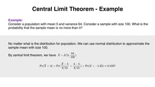
Central Limit Theorem - Example
Example:
Consider a population with mean 5 and variance 64. Consider a sample with size 100. What is the
probability that the sample mean is no more than 4?
No matter what is the distribution for population. We can use normal distribution to approximate the
sample mean with size 100.
By central limit theorem, we have
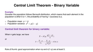
Central Limit Theorem - Binary Variable
Example:
Consider the population follows Bernoulli distribution, which means that each element in the
population is ether 0 or 1, the probability of having 1 (success) is p.
o Population mean
o Population variance
Central limit theorem for binary variable:
When n gets large, we have
or
Rule of thumb: good approximation when np and n(1−p) are at least 5.
Central Limit Theorem - Binary Variable
Comparison between binomial distribution and its normal approximation:
n=1 n=2 n=5
n=10 n=30 n=100
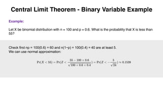
Central Limit Theorem - Binary Variable Example
Example:
Let X be binomial distribution with n = 100 and p = 0.6. What is the probability that X is less than
55?
Check first np = 100(0.6) = 60 and n(1−p) = 100(0.4) = 40 are at least 5.
We can use normal approximation:

Lecture7 - Sampling Distribution - 0923.pdf

  • 1.
    Agenda Statistical Analysis forBusiness Decisions 02 Central Limit Theorem 01 Law of Large Number o Population and sample o Property of sample mean o Approximation of sample mean
  • 2.
    Recap - DiscreteRandom Variable Bernoulli Mean Variance PMF Binomial Poisson o Count of successes for repeated discrete trials o Count of events over a continuous time o Binomial approaches Poisson when n is really large and p is really small o Can be used to approximate binomial and is easy to calculate, because has only 1 parameter o Binary outcome Euler constant = 2.718
  • 3.
    Recap - ContinuousRandom Variable Exponential Mean Variance PDF Normal o Time between independent random events o Poisson: event count -> exponential: time between events o Memoryless property For exponential distribution, we have e.g., the life of a light bulb
  • 4.
    Population and Sample Population oObjects we would like to know o e.g., age and incomes of individuals in a city, satisfaction level of consumers Sample o Subset of population Goal of Inference Use representative sample (small picture) to make an educated guess on the population (big picture)
  • 5.
    Population and Sample Population orepresented by bar chart/histogram o summarized by (relative) frequency table f(x) o mean: μ; variance: σ2 Sample o an observation from population Random Sample o A random draw from population o A random variable with probability function is the same as frequency table f(x) o For a sample with a size n, we write X1, X2, . . . , Xn
  • 6.
    Simple Random Sample- Definition Simple Random Sample: most basic random sample o Each element has equal probability being selected. o Each element is selected independently Explanation: X1, …, Xn is a simple random sample if o X1, … , Xn are independent random variables, and o X1, . . . , Xn follow the same probability function P(x) or f(x) Probability mass function Probability density function
  • 7.
    Simple Random Sample- Property Property of Simple Random Sample: If X1, …, Xn is a simple random sample, then o o o Consider a population with mean μ and variance σ2. Simple random sample in fact has an even strong property Each observation follows the same distribution as the population This includes all summary statistics
  • 8.
    Other Sampling Methods Simplerandom sample is simple but difficult to achieve in practice: o Online surveys likely exclude seniors who do not use internet often o Samples from offline surveys are likely to be dependent due to geographical correlation (e.g., economic condition, location preference) o Advanced sampling method to reduce sampling error: Stratified sampling - divide population into subsamples, and do simple random sample within each subsample, and produce weighted average across subsamples
  • 9.
    Statistics - Definition Statistics: Afunction of a sample X1, ... Xn o Data summary o Data reduction (simplification) Examples: sample mean, sample variance
  • 10.
    Sample Mean -Definition Sample mean: Sample mean is the mean of a sample. o This varies sample by sample o Sample mean is also a random variable. It is useful to guess population mean Hence, we can also derive expectation, variance for the sample mean.
  • 11.
    Sample Mean -Expectation Expectation of sample mean: Expectation of sample mean is population mean Intuition: o If we sample many times, average of all sample means is the population mean o This nice property is known as unbiasedness (see next chapter)
  • 12.
    Sample Mean -Expectation Average of sample means: Rolling a dice for (infinitely) many times Amy rolls a dice for 5 times Charlie rolls a dice for 10 times Mean for Amy's sample (5 results) Mean for Charlie's sample (10 results)
  • 13.
    Sample Mean -Expectation Example Example: Consider population has three numbers: 1, 2, and 3, each with the same probability. x1x2 1 2 3 1 1 1.5 2 2 1.5 2 2.5 3 2 2.5 3 The sample size can be larger, and even larger than 3, and there are more possibilities. o Population mean​ o Consider sample with size=1, the sample mean can be one of {1,2,3} with the same probability. Expectation of the sample mean for size=1 is​ o Consider sample with size=2, the sample mean can be one of the following 9 results with the same probability. Expectation of the sample mean for size=2 is​
  • 14.
    Sample Mean –Expectation Proof Linear property of expectation Expectation of sum = sum of expectation
  • 15.
    Sample Mean -Variance Variance of sample mean: Population variance divided by sample size: Standard error of sample mean: Standard deviation of the sample mean: It is not the sample variance! Standard deviation of a statistics is often called standard error
  • 16.
    Sample Mean -Variance Example Example: Consider population has three numbers: 1, 2, and 3, each with the same probability. o Population mean Population variance o Consider sample with size=1, the expectation of the sample mean is . Therefore, the variance of sample mean is o Consider sample with size=2, . Therefore, the variance of sample mean is x1x2 1 2 3 1 1 1.5 2 2 1.5 2 2.5 3 2 2.5 3
  • 17.
    Sample Mean –Variance Proof Transformation of variance Variance of sum = sum of variance if independent
  • 18.
    Sample Mean –Large Samples When sample size gets larger, o As sample size n enlarges, the variance of sample mean shrinks o Moreover, variance vanishes as n goes to infinity, that is, o As , when n gets larger, we have the sample mean eventually very close to population mean, that is,
  • 19.
    Law of LargeNumbers Law of large numbers: For any , when n is sufficiently large, we have Or more rigorously, Let X1, . . . , Xn be a random sample from a distribution with mean μ and variance σ2. Loosely speaking, when sample size is large, variation disappears and the sample mean becomes population mean. Or, with a larger sample, sample mean is closer to population mean, and it can be as close as we want.
  • 20.
    Law of LargeNumber Markov inequality Consider a nonnegative random variable, , then for all t>0, Hence, we get the Markov inequality Chebyshev inequality Consider , then by Markov inequality Hence, we get Chebyshev inequality
  • 21.
    Law of LargeNumber As we have Chebyshev inequality Then, since , we have Taking the limit on both sides, we arrive at the law of large number.
  • 22.
    Sample Mean –Large Samples When sample size gets larger, o Law of large numbers says that sample mean is eventually close to μ. o But, sample mean itself is still a random variable. What is the distribution function of sample mean when n becomes larger? Always normal distribution, regardless of how population looks like The distribution of sample mean RATHER THAN the distribution of a sample itself
  • 23.
    Sample Mean -Variance Example Example: Consider population has three numbers: 1, 2, and 3, each with the same probability. Let's look at the CDF of the sample mean for different sample sizes. Normal distribution n=1 n=2 n=10 n=100 n=1000 n=10000
  • 24.
    Central Limit Theorem Centrallimit theorem: sample mean approximately follows a normal distribution with a large enough sample. When n gets large, we have or Rule of thumb: sample size n is at least 35.
  • 25.
    Central Limit Theorem- Example Example: Consider a population with mean 5 and variance 64. Consider a sample with size 100. What is the probability that the sample mean is no more than 4? No matter what is the distribution for population. We can use normal distribution to approximate the sample mean with size 100. By central limit theorem, we have
  • 26.
    Central Limit Theorem- Binary Variable Example: Consider the population follows Bernoulli distribution, which means that each element in the population is ether 0 or 1, the probability of having 1 (success) is p. o Population mean o Population variance Central limit theorem for binary variable: When n gets large, we have or Rule of thumb: good approximation when np and n(1−p) are at least 5.
  • 27.
    Central Limit Theorem- Binary Variable Comparison between binomial distribution and its normal approximation: n=1 n=2 n=5 n=10 n=30 n=100
  • 28.
    Central Limit Theorem- Binary Variable Example Example: Let X be binomial distribution with n = 100 and p = 0.6. What is the probability that X is less than 55? Check first np = 100(0.6) = 60 and n(1−p) = 100(0.4) = 40 are at least 5. We can use normal approximation: