Transfer Function In Sensor

1. Transfer Function in
Sensors
Kholis Nurhanafi

2. Introduction
• Sensors convert non-electrical stimuli into electrical
signals.
• The transfer function describes the relationship
between stimulus (input) and electrical signal
(output).
• Main goal: Determine the stimulus from the electrical
signal produced by the sensor.
• Understanding the transfer function enhances sensor
performance in various applications.

3. Definition of Transfer Function
• A static transfer function is an input-output relationship that does not
change over time.
• General notation:
• is the electrical output of the sensor (voltage, current, etc.).
• is the measured input stimulus.
• An ideal transfer function ensures the sensor produces accurate and reliable
output.

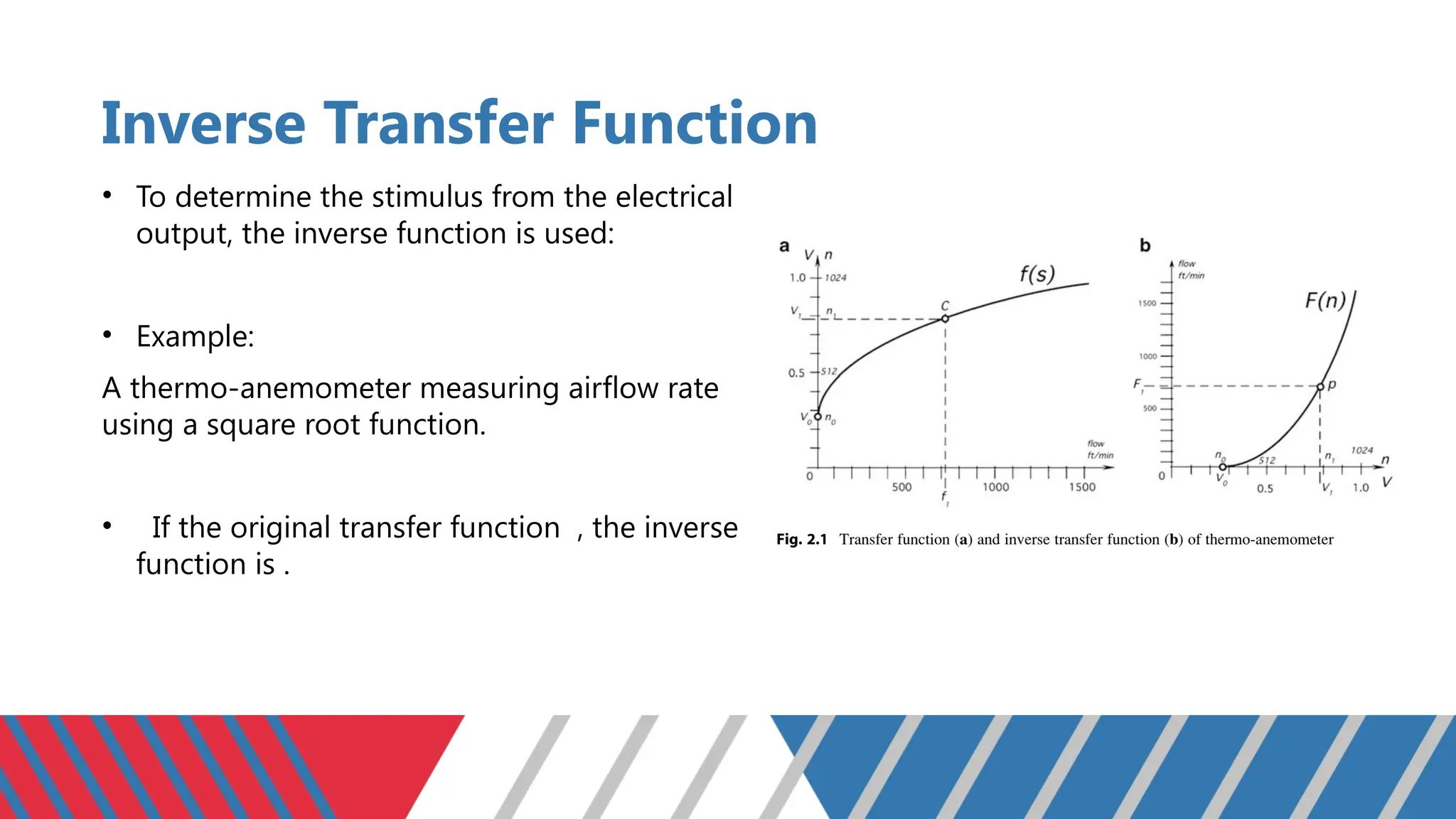
4. Inverse Transfer Function
• To determine the stimulus from the electrical
output, the inverse function is used:
• Example:
A thermo-anemometer measuring airflow rate
using a square root function.
• If the original transfer function , the inverse
function is .

5. Mathematical Model of Transfer Function
• A mathematical model formally represents the input-output
relationship of a sensor.
• Models can be in the form of:
1) Value tables.
2) Graphs depicting stimulus-output relationships.
3) Explicit mathematical equations.
• If the transfer function does not change over time, it is called a static
transfer function.
• Common mathematical models include linear, exponential,
logarithmic, and polynomial equations.

6. Example of a Linear Transfer Function
- A linear model represents a direct relationship between stimulus and
output:
is the intercept, the output value when the input is zero.
is the sensor sensitivity (slope of the graph).
- Example:
1. A resistive potentiometer for position measurement.
2. Temperature sensors based on RTDs (Resistance Temperature Detectors).

7. Example of a Linear Transfer Function

8. Linear Transfer Function with Reference
- If a reference is used, the transfer function becomes:
are the reference input-output points.
- The inverse transfer function is:
-
Used in sensors with a reference point, such as force sensors with zero calibration

9. Example of a Nonlinear Transfer Function
- Many sensors exhibit nonlinear transfer functions, such as:
Logarithmic:
Exponential:
Power function:
- Examples:
1. Light sensors based on photodiodes.
2. Thermistors for temperature measurement.

12. Approximation Approaches for Transfer
Functions
- Not all sensors have explicit mathematical models.
- Approximation methods include:
a) Linear regression for nearly linear functions.
b) Polynomial approximation for nonlinear relationships.
c) Piecewise linear approximation for unpredictable behavior.
- Used for sensors with complex characteristics.

13. Linear Regression for Approximation
- If the sensor relationship is not exact, use linear regression:
- is the number of measurements.
- Applied in pressure or humidity sensors.

14. Polynomial Approximation
- If data does not fit basic functions, use polynomials:
- Example applications:
- Gas sensors with nonlinear concentration-output voltage relationships.
• Polynomial approximation is useful when sensor responses cannot be accurately described by
simple equations.
• Higher-order polynomials can provide better approximations but may increase computational
complexity.
• The best choice of polynomial order depends on the required accuracy and available
computational resources.

15. Sensor Sensitivity
• - Sensitivity is defined as the first derivative of the transfer function:
• In nonlinear sensors, sensitivity varies across the stimulus range.
• High sensitivity means small changes in stimulus result in large changes in
output.

16. Piecewise Linear Approximation
• Divides a nonlinear transfer function into multiple linear segments.
• Each segment is defined by a simple linear equation.
• Used in: pressure sensors with nonlinear output.

18. Considerations for Piecewise
Approximation
• It makes sense to select knots only for the input range of interest (span) to reduce
complexity.
• The error of a piecewise approximation is characterized by a maximum deviation from the
real curve.
• The larger the deviation , the greater the number of segments needed to maintain
accuracy.
• Knots should be closer in regions of high nonlinearity and further apart where the
function is more linear.
• The signal processor must store knot coordinates in memory and perform linear
interpolation to compute the input stimulus .

19. Spline Interpolation
• Uses piecewise polynomials to create smoother curves.
• Example: Temperature sensors where data needs interpolation over a wide
range.

20. Multidimensional Transfer Functions
• Some sensors depend on more than one input variable.
• Example:
- A humidity sensor's output depends on both humidity and temperature.
- An infrared thermal radiation sensor follows the Stefan-Boltzmann law.
The transfer function of an infrared sensor involves two temperature variables:
, the absolute temperature of an object of measurement and , the absolute
temperature of thesensing element.
•

22. Calibration
• Calibration is required to enhance sensor accuracy by correcting deviations.
• It involves applying known stimuli and measuring the corresponding output.
• Methods of calibration:
• Modifying the transfer function: Compute new coefficients to fit experimental data, ensuring a
unique transfer function without modifying the sensor.
• Adjusting the data acquisition system: Modify output signals to fit a normalized transfer
function (e.g., scaling and shifting data).
• Modifying sensor properties: Physically alter the sensor to match a predetermined transfer
function.
• Using sensor-specific reference devices: Employ a matching reference to compensate for
inaccuracies.
• Example: Thermistor calibration methods using controlled liquid baths and precision thermometers.

24. Conclusion
• Transfer functions are fundamental in sensor
analysis.
• Approximation methods enhance measurement
accuracy.
• Understanding transfer functions aids in
designing better sensor systems.
• Modern sensors often use nonlinear approaches
and calibration for improved accuracy.

25. Reference

26. Thank you
Everything is controlled by probabilities.
I would like to know—who controls probabilities?
Stanisław Jerzy Lec
Polish Poet