Downloaded 17 times


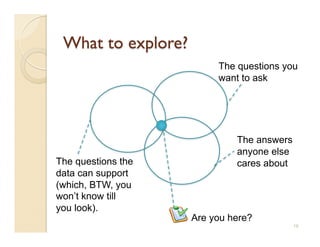
![ Does the pace of change in modern software engineering make GQM impractical?
◦ Researchers need rapid adaptation methods to keep up with this faster pace. Otherwise…
Basili’s SEL’s learning organization experiment lasted ten years (from 1984 to 1994) during a
period of relative stability within the NASA organization.
Starting in 1995, the pace of change within NASA increased dramatically.
◦ New projects were often outsourced
◦ SEL became less the driver and more the observer, less proactive and more reactive.
◦ Each project could adopt its own structure.
◦ SEL-style experimentation became difficult: no longer a central model to build on.
NASA also tried some pretty radical development methods
◦ ‘Faster, Better, Cheaper” lead led to certain high profile errors which were attributed to
production haste, poor communications, and mistakes in engineering management.
◦ When ‘Faster, Better, Cheaper’ ended, NASA changed, again, their development practices.
This constant pace of change proved fatal to the SEL.
◦ Basili el al. [24] describe the period 1995-2001 as one of ‘retrenchment’ at the SEL.
14](https://image.slidesharecdn.com/locallessons-100704045406-phpapp02/85/Learning-Local-Lessons-in-Software-Engineering-14-320.jpg)
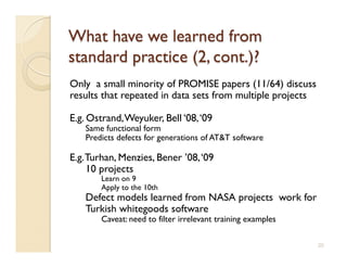
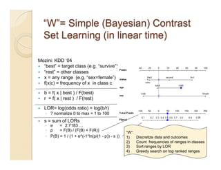
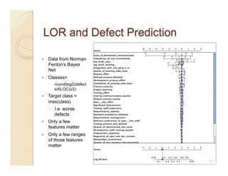
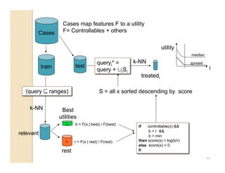


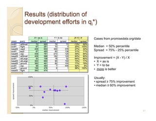

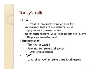
This document discusses issues with seeking general theories in software engineering research. It argues that the goal should be seeking local lessons rather than general theories, as external validity has proven elusive. "W" is proposed as a baseline tool for generating local lessons from empirical studies. The document also discusses challenges to the validity of prior results from reanalyzing old data with new techniques and finding issues that challenge previous conclusions. Only a small portion of papers from one conference discussed results that repeated across multiple projects.


