Download to read offline
![7/25/2022 13
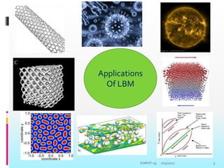
EVOLUTION OF PARTICLE DISTRIBUTION
FUNCTION IN LBE
STREAMING
)
,
(
)
,
( t
x
f
t
t
t
c
x
f k
k
k
COLLISION
)]
,
(
)
,
(
[
1
)
,
(
)
,
( t
x
f
t
x
f
t
x
f
t
x
f k
eq
k
k
k
13
ICMFHT-19](https://image.slidesharecdn.com/krunallbm-220725054459-9da28faa/85/Krunal_lbm-pptx-12-320.jpg)
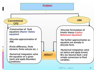

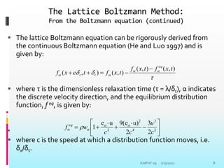
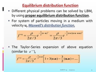
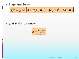
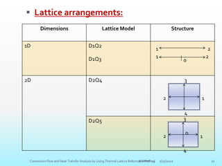
The document provides an introduction to the lattice Boltzmann method (LBM). It discusses that LBM is a kinetic method based on solving the Boltzmann equation for the particle distribution function. The lattice Boltzmann equation can be derived from the continuous Boltzmann equation. LBM involves discretizing the particle distribution function in velocity space and streaming and colliding particles on a lattice. It offers advantages over conventional CFD methods like easier treatment of complex boundaries and multi-phase flows.