Kinematically_exact_curved_and_twisted_strain-based_beam.pdf

1. Kinematically exact curved and twisted strain-based beam P. Češarek, M. Saje, D. Zupan ⇑ University of Ljubljana, Faculty of Civil and Geodetic Engineering, Jamova 2, SI-1115 Ljubljana, Slovenia a r t i c l e i n f o Article history: Received 3 July 2011 Received in revised form 13 December 2011 Available online 6 April 2012 Keywords: Strain measure Constant strain Non-linear beam theory Three-dimensional beam Three-dimensional rotation a b s t r a c t The paper presents a formulation of the geometrically exact three-dimensional beam theory where the shape functions of three-dimensional rotations are obtained from strains by the analytical solution of kinematic equations. In general it is very demanding to obtain rotations from known rotational strains. In the paper we limit our studies to the constant strain field along the element. The relation between the total three-dimensional rotations and the rotational strains is complicated even when a constant strain field is assumed. The analytical solution for the rotation matrix is for constant rotational strains expressed by the matrix exponential. Despite the analytical relationship between rotations and rotational strains, the governing equations of the beam are in general too demanding to be solved analytically. A finite-element strain-based formulation is presented in which numerical integration in governing equations and their variations is completely omitted and replaced by analytical integrals. Some interesting connections between quantities and non-linear expressions of the beam are revealed. These relations can also serve as useful guidelines in the development of new finite elements, especially in the choice of suitable shape functions. Ó 2012 Elsevier Ltd. All rights reserved. 1. Introduction Beam elements have played a very important role in modeling engineering structures. Their applicability is, however, strongly dependent on the accuracy, robustness and efficiency of the numerical formulation. This is particularly important in studying initially curved and twisted beams, which are well known to differ considerably in their behavior with respect to straight elements. That is why the mathematical modeling of initially curved and twisted beams has been a special subject of research both in past and at present, see, e.g. the recent publications by Atanackovic and Glavardanov (2002), Atluri et al. (2001), Gimena et al. (2008), Kapania and Li (2003), Kulikov and Plotnikova (2004), Leung (1991), Sanchez-Hu- bert and Sanchez Palencia (1999), Yu et al. (2002). Among various existing non-linear beam theories Reissner’s ‘geometrically exact finite-strain beam theory’ (Reissner, 1981) is the most widely used one. Several finite-element formulations have been proposed for the numerical solution of its governing equations, see, e.g. Cardona and Géradin (1988), Ibrahimbegovic (1995), Jelenić and Saje (1995), Ritto-Corrêa and Camotim (2002), Schulz and Filippou (2001), Simo and Vu-Quoc (1986), to list just a few among the more often cited works. Another important issue in any finite element formulation is the choice of the primary interpolated variables. Most of the above cited approaches use displacements and rotations or solely rotations as the interpolated degrees of freedom. Because the spatial rotations are elements of the multiplicative SOð3Þ group, the configuration space of the beam is a non-linear manifold. That is why the way the rotations are parametrized and interpolated is crucial. In the displacement-rotation-based formulations, the eval- uation of strains, internal forces and moments requires the differentiation of the assumed kinematic field which decreases the accuracy of the differentiated quantities compared to the primary interpolated variables which might be very important in materially non-linear problems. By contrast, if the strains are taken to be the interpolated variables, the additive-type of interpolation can be used without any restrictions. By such an approach the determination of internal forces and moments do not require the differentiation. Instead, the fundamental problem of a strain-based formulation now becomes the integration of rotations from the given interpolated strains. In the three dimensions, the derivative of the rotations with respect to parameter equals the product of a rotation-dependent non-linear transformation matrix and the rotational strain. In general such a system of differential equations cannot be integrated in a closed form. This is probably the main reason why, in the three-dimensional beam theories, the total strain field or even solely the rotational strain is very rarely chosen as the primary var- iable. Some authors integrate the strain–displacement relations and employ the results for proposing a more suitable interpolation for the three-dimensional rotations. Tabarrok et al. (1988) assumed an analytically integrable curvature distribution to develop a more suitable interpolation for displacements and rotations in 0020-7683/$ - see front matter Ó 2012 Elsevier Ltd. All rights reserved. http://dx.doi.org/10.1016/j.ijsolstr.2012.03.033 ⇑ Corresponding author. Tel.: +386 1 47 68 632; fax: +386 1 47 68 629. E-mail address: dejan.zupan@fgg.uni-lj.si (D. Zupan). International Journal of Solids and Structures 49 (2012) 1802–1817 Contents lists available at SciVerse ScienceDirect International Journal of Solids and Structures journal homepage: www.elsevier.com/locate/ijsolstr

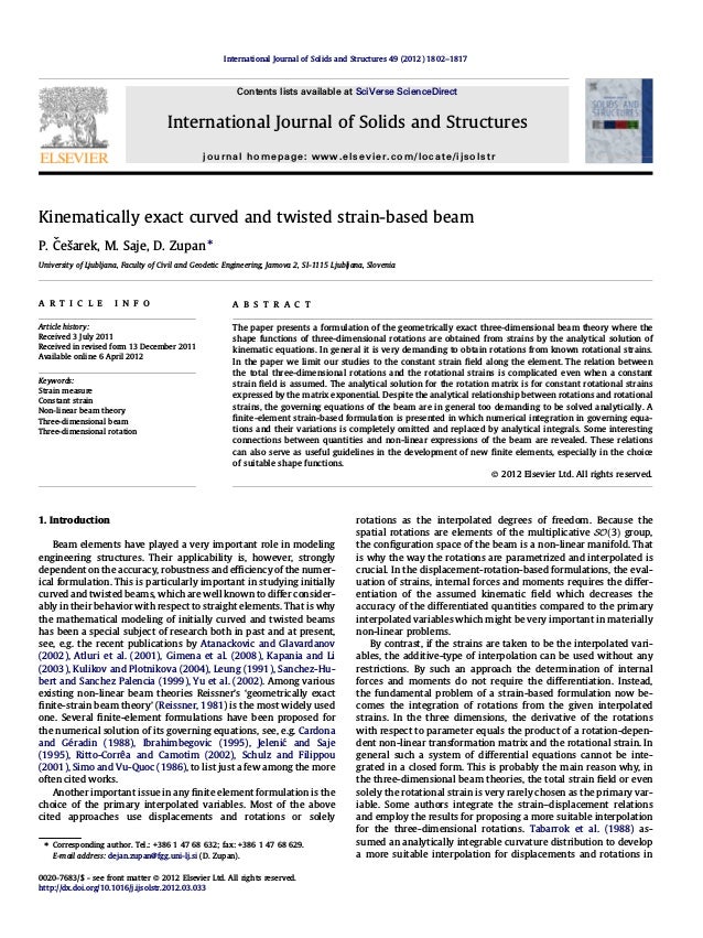
2. order to describe properly the rigid-body modes of arbitrarily curved and twisted beam. Choi and Lim (1995) employed the solution of the linearized strain–displacement relations to obtain the finite-elements for constant and linear shape of varied strains. Schulz and Filippou (2001) proposed an interesting non-linear Timoshenko beam element where the displacements and both the infinitesimal (incremental) curvatures and the infinitesimal rotations are interpolated. In Schulz and Filippou (2001) the reduced integration has to be used to avoid shear locking. Santos et al. (2010) introduced a hybrid-mixed formulation in which the stress-resultants, the displacements and the rotations are taken as independent variables. The pure strain-based formulation was proposed by Zupan and Saje (2003) who developed the spatial beam finite-element formulation of the Reissner–Simo beam theory in which the total strain vectors are the only interpolated variables. Such a formulation is locking-free, objective and a standard additive-type of interpolation of an arbitrary order is theoretically consistent and can be used for both total strains and their variations. In Zupan and Saje (2003) a numerical method (the Runge– Kutta method) is used for the integration of the total rotations from the given total rotational strains, which is due to the complicated form of the kinematical equations. It has already been noted in the analysis of planar frames that the strain-based beam formulations are numerically efficient and well applicable in various problems. In particular, applications of the strain-based elements to the dynamics (Gams et al., 2007), and to the statics of the reinforced concrete frame with the strain localization (Bratina et al., 2004) and the reinforced concrete frame in fire (Bratina et al., 2007) show the advantages of both higher- order and a simple constant strain element. The constant-strain elements are especially important for the efficient numerical modeling of strain-softening in concrete. The same should equally apply to the three-dimensional beam structures. In the paper we follow and extend the ideas of the planar case and develop a robust and efficient three-point finite element with 24 degrees of freedom based on Reissner’s beam theory. In order to obtain an exact analytical solution for the rotations in terms of the rotational strain, we limit our studies to the constant strain field along the element. It is important to point out that integrating the constant strain field results in a non-linear, linked form of rotations and displacements. This immediately suggests that the classical additive-type of interpolation of the rotation and displacement field, in which the displacements are interpolated by using only nodal displacements, and the rotations only nodal rotations, is not the most natural choice. This has also been observed by Borri and Bottasso (1994) by using the helicoidal approximation, and by Jelenić and Papa (2011) who studied the genuine linked interpolation functions for the three-dimensional linearized Timoshenko beams. In contrast to Borri and Bottasso (1994) and Jelenić and Papa (2011), the finite-element formulation employed here is based on the strain field rather than on the displacement-rotation field, which results in different types of finite elements and considerable differences in the overall numerical implementation. The analytical relationship between the rotations and the rotational strains is given in the exact analytical form, which enables us to perform the integration in governing equations and their variations analytically. An interesting observation then follows that the analytical approach, although based on the assumption of the constant strain field over the finite element, suggests the integrals must be decomposed into the total rotational operator at the end-point of the beam and the arc-length dependent operator along the beam. A special study is made in searching the form of these operators and their similarity with respect to the Rodrigues formula. The similarity between the terms is also exploited to re- duce the computational cost of the proposed algorithm. The results can serve as useful guidelines for choosing suitable shape functions for various quantities in the development of new, higher-order interpolation beam formulations. The present finite element is free of any numerical integration or numerical differentiation error, the only error of the element being the assumed strain field. One of distinguishing characteristics of the present element is the mathe- matically proved convergence of the discrete solution to the exact one by reducing the element length. This means that a sufficiently fine mesh of the present elements give accurate results of the geometrically and materially non-linear beam theory without any lim- itations set on the magnitude of rotations, displacements and strains. The efficiency and the accuracy of the proposed approach is demonstrated by numerical examples. 2. Geometry, rotations and skew-symmetric matrices The geometrically exact finite-strain beam theory assumes that an arbitrary configuration of the beam is described by (see Fig. 1): (i) The position vector r * ðxÞ of the beam axis, and (ii) The orthonormal base vectors G * 1ðxÞ; G * 2ðxÞ; G * 3ðxÞ attached to the planes of the cross-sections. ‘‘x’’ is the arc-length parameter of the centroidal axis of the beam axis connecting the centroids, C, of the cross-sections in the undeformed configuration, vectors G * 2ðxÞ and G * 3ðxÞ point along the principal axes of inertia of the cross-section, and G * 1ðxÞ is its normal: G * 1 ¼ G * 2 G * 3. Note that G * 1 is generally not colinear with the tangent to the beam axis, d r * dx (Fig. 1). Vectors G * 1ðxÞ; G * 2ðxÞ; G * 3ðxÞ define the basis of the local coordinate system. We further introduce a reference point O and a triad of fixed orthonormal base vectors g * 1; g * 2; g * 3 n o , which define the global coordinate system (X,Y,Z). The relationship between the local and the global bases is represented by rotation matrix R(x). Abstract vectors have to be expressed with respect to any basis to obtain their component (coordinate) representations, here marked by a bold-face font, and equipped with an index denoting the basis used. The coordinate transformation between two component forms of a vector v * is represented by the rotation matrix: vg ¼ RvG: ð1Þ For the parametrization of the three-dimensional rotations, we here employ the rotational vector #g (Argyris, 1982) whose length equals the angle of rotation and its direction is colinear with the axis of rotation. If we introduce a skew-symmetric matrix H H ¼ 0 #3 #2 #3 0 #1 #2 #1 0 2 6 4 3 7 5; ð2Þ composed from components {#1,#2,#3} of the vector #g, the rotation matrix is expressed by the Rodrigues formula Fig. 1. Model of the three-dimensional beam. P. Češarek et al. / International Journal of Solids and Structures 49 (2012) 1802–1817 1803

3. R ¼ I þ sin # # H þ 1 cos # #2 H2 ; ð3Þ where I is the identity matrix, and # ¼ k#gk ¼ ffiffiffiffiffiffiffiffiffiffiffiffiffiffiffiffiffiffiffiffiffiffiffiffiffiffiffi #2 1 þ #2 2 þ #2 3 q . An alternative to the Rodrigues formula for the rotation matrix is the matrix exponential: R ¼ I þ H þ 1 2! H2 þ 1 3! H3 þ þ 1 n! Hn ¼ expðHÞ; ð4Þ which can be found more convenient to employ in some cases. Note also that Hu ¼ # u; ð5Þ for every u, which means that the cross vector product # u can be replaced by the matrix product Hu whenever needed. The above holds for arbitrary two vectors. It is thus suitable to introduce the skew-symmetric operator S, which maps an arbitrary vector into the skew-symmetric matrix S(v): S : v # SðvÞ SðvÞ ¼ 0 v3 v2 v3 0 v1 v2 v1 0 2 6 4 3 7 5: ð6Þ Vector v is called the axial vector of the skew-symmetric matrix S(v). 3. Strain vectors, equilibrium and constitutive equations The geometrically exact finite-strain beam theory introduces two strain vectors (Reissner, 1981): (i) the translational strain vector cG, and (ii) the rotational strain vector jG. When expressed with respect to the local basis, their components have physical interpre- tation: cG1 is the extensional strain, cG2 and cG3 are shear strains; jG1 is the torsional strain, jG2 and jG3 are the bending strains (curvatures). The relations between the strains, displacements and rotations are derived from the condition that the strains and stresses are consistent with the virtual work principle for any internal forces and any magnitude of deformation. This condition yields the following relationships between the variations of kinematic vector variables (rg,#g) and the variations of strain vectors (cG,jG) dcG ¼ RT dr0 g d#g r0 g ; ð7Þ djG ¼ RT d#0 g: ð8Þ By integrating Eqs. (7) and (8) with respect to the variations and following the approach of Reissner (1981), we obtain the relation between the strain measures, displacements and rotations: cG ¼ RT r0 g þ cG; ð9Þ jG ¼ TT #0 g þ dG; ð10Þ where TT ¼ I 1 cos # #2 H þ # sin # #3 H2 is the transformation matrix between jG and #0 g. Note that the integration is not straightforward due to different bases in which the relative variations of strain and rotational vectors are introduced. For the details of the derivation, see, e.g. Ibrahimbegovic (1997). Vector functions cG(x) and dG(x) are the unknown variational constants, which we have to express with the known strain and kinematic fields in the initial state of the beam. cG and dG are, in a general case, dependent on x, yet they do not change during the deformation of the beam. From (9) and (10) it follows that any sufficiently smooth initial state of strain can be applied, which is sufficient to describe practically any initially curved and twisted beam. The equilibrium equations of an infinitesimal element of a beam are given by the following set of differential equations: ng ¼ N0 g; ð11Þ mg ¼ M0 g r0 g Ng: ð12Þ The two stress resultants, the force Ng and the moment Mg, depend both on the external distributed force and moment vectors ng and mg per unit of the undeformed length of the axis, and on the deformed shape of the axis, described by its position vector rg. On the other hand, the stress resultants are dependent on strain vectors cG and jG as determined by the constitutive equations NG ¼ CN cG; jG ð Þ; ð13Þ MG ¼ CM cG; jG ð Þ: ð14Þ 4. Governing equations of the strain-based formulation The complete set of the beam equations consists of the constitutive Eqs. (13) and (14), the equilibrium Eqs. (11) and (12) and the kinematic Eqs. (9) and (10) set with respect to the global basis: RCNðcG; jGÞ Ng ¼ 0; ð15Þ RCMðcG; jGÞ Mg ¼ 0; ð16Þ N0 g þ ng ¼ 0; ð17Þ M0 g þ mg SðNgÞRðcG cGÞ ¼ 0; ð18Þ r0 g RðcG cGÞ ¼ 0; ð19Þ #0 g TT ðjG dGÞ ¼ 0: ð20Þ The related static boundary conditions are: S0 þ Ngð0Þ ¼ 0; ð21Þ P0 þ Mgð0Þ ¼ 0; ð22Þ SL NgðLÞ ¼ 0; ð23Þ PL MgðLÞ ¼ 0: ð24Þ Here, S0 , P0 , SL , PL are vectors of the external point loads at the boundaries x = 0 and x = L. In (18) the use of the skew-symmetric matrix S replaces the vector product (see Eq. (5)). Eqs. (17)–(20) constitute a system of four first-order ordinary differential equations. If we assume that ng, mg, cG and jG are known analytic functions of x, the formal solutions of these equations read NgðxÞ ¼ Ngð0Þ Z x 0 ngð~ xÞd~ x; ð25Þ MgðxÞ ¼ Mgð0Þ þ Z x 0 ½SðNgð~ xÞÞRð~ xÞðcGð~ xÞ cGð~ xÞÞ mgð~ xÞd~ x; ð26Þ rgðxÞ ¼ r0 g þ Z x 0 Rð~ xÞðcGð~ xÞ cGð~ xÞÞd~ x; ð27Þ #gðxÞ ¼ #0 g þ Z x 0 TT ð~ xÞðjGð~ xÞ dGð~ xÞÞd~ x: ð28Þ Eqs. (25) and (26) are evaluated at x = L and inserted in the static boundary conditions at the right boundary of the beam. The fulfilment of the displacement and rotation boundary conditions at x = L places additional requirements on strain vectors: rgðLÞ r0 g Z L 0 RðxÞðcGðxÞ cGðxÞÞdx ¼ 0; ð29Þ #gðLÞ #0 g Z L 0 TT ðxÞðjGðxÞ dGðxÞÞdx ¼ 0: ð30Þ 1804 P. Češarek et al. / International Journal of Solids and Structures 49 (2012) 1802–1817

4. Once Eqs. (17)–(20) have been solved by the integration, see Eqs. (25)–(28), the complete set of the equations of the strain-based formulation of the geometrically exact three-dimensional beam then consists of the algebraic Eqs. (15) and (16), the kinematic conditions (29) and (30) and the static boundary conditions (21)–(24): f 1 ¼ RCNðcG; jGÞ Ng ¼ 0; ð31Þ f 2 ¼ RCMðcG; jGÞ Mg ¼ 0; ð32Þ f 3 ¼ rL g r0 g Z L 0 RðcG cGÞdx ¼ 0; ð33Þ f 4 ¼ #L g #0 g Z L 0 TT ðjG dGÞdx ¼ 0; ð34Þ f 5 ¼ S0 g þ N0 g ¼ 0; ð35Þ f 6 ¼ P0 g þ M0 g ¼ 0; ð36Þ f 7 ¼ SL g N0 g þ Z L 0 ng dx ¼ 0; ð37Þ f 8 ¼ PL g M0 g Z L 0 SðNgÞRðcG cGÞ mg dx ¼ 0: ð38Þ Eqs. (31)–(38) along with the auxiliary relations (25)–(28) constitute the set of eight equations for eight unknowns: (i) boundary kinematic vectors r0 g ; #0 g ; rL g; #L g, (ii) boundary equilibrium stress resultants N0 g ; M0 g , and (iii) strain vector functions cG(x) and jG(x). Formulation (31)–(38) thus employs the strains as the only unknown functions of x. The system of Eqs. (31)–(38) is in general too demanding to be solved analytically. The approach where the strain vectors are approximated by an arbitrary order interpolation and the kinematic vectors obtained by the numerical integration based on (27) and (28) was presented by Zupan and Saje (2003). In the present paper, our goal is to avoid the numerical integration along the beam element completely. This is achieved by assuming that the strains are constant. 5. Constant strain finite-element formulation Let X denote the given skew-symmetric matrix composed from the components of the curvature vector jG (X = S(jG)). Its definition (Argyris, 1982): X ¼ RT R0 represents a linear differential equation for R(x). When the skew- symmetric matrix X is independent of x, and thus the curvature vector jG constant, the analytical solution can be found from the following result. Let jG be the constant curvature vector and X = S(jG) the corresponding skew-symmetric matrix. Then RðxÞ ¼ R0RðxjGÞ ¼ R0 expðxSðjGÞÞ ð39Þ is the solution of the initial value problem R0 ðxÞ ¼ RðxÞX; Rð0Þ ¼ R0: Here RðxjGÞ denotes the exponential map (see Eq. (4)) composed from skew-symmetric matrix xS(jG), i.e. RðxjGÞ ¼ I þ xSðjGÞ þ 1 2! x2 S2 ðjGÞ þ þ 1 n! xn Sn ðjGÞ þ Proof. The proof is straightforward, if the exponential form (4) of the rotation matrix is employed. The differentiation of the presumed solution with respect to x gives R0 ðxÞ ¼ R0 d dx RðxjGÞ: The derivative of RðxjGÞ with respect to x is (see (4) and (6)): d dx RðxjGÞ ¼ d dx I þ xSðjGÞ þ 1 2! x2 S2 ðjGÞ þ þ 1 n! xn Sn ðjGÞ þ ¼ SðjGÞ þ xS2 ðjGÞ þ 1 2! x2 S3 ðjGÞ þ þ 1 ðn 1Þ! xn1 Sn ðjGÞ þ ¼ I þ xSðjGÞ þ 1 2! x2 S2 ðjGÞ þ þ 1 ðn 1Þ! xn1 Sn1 ðjGÞ þ SðjGÞ ¼ RðxjGÞSðjGÞ: Thus, R0 ðxÞ ¼ R0RðxjGÞSðjGÞ ¼ RðxÞX: By evaluating R(x) at x = 0, we obtain Rð0Þ ¼ R0Rð0jGÞ ¼ R0I ¼ R0: This concludes the proof. h In standard approaches only infinitesimal and/or incremental rotational vectors are allowed to be interpolated due to the non-lin- earity of three-dimensional rotations. A standard beam element with a linearly interpolated incremental rotational vector would thus also result in constant strains but with only an approximate total rotation field. In contrast, the exact rotation field is obtained here. The solution (39) shows that the total rotational operator is the product of the rotation at the boundary point of the beam, x = 0, and the relative arc-length, x, dependent rotation. This multiplicative decomposition is also inherited by the linearization, as shown in Appendix A, and thus seems to be natural. The idea of expressing the rotations with respect to the local coordinate system attached to a point on the element is typical for the co-rotational beam elements, see, e.g. Crisfield (1990), Battini and Pacoste (2002). Such a decomposition of rotations was also used in the rotation interpolation by Crisfield and Jelenić (1999) to obtain the strain-objective numerical formulation of the geometrically exact beam. It is now obvious that the rotation boundary condition (34) can be substituted by a direct (not integral) expression. Once the rotation matrix R(x) is at hand, we are able to extract the components of the corresponding rotational vector #g(x) at any point x. Due to its numerical stability, the Spurrier algorithm (Spurrier, 1978) is used. The algorithm, however, cannot be expressed as an explicit function of the components of R(x). Therefore, we will use the sym- bolic notation #gðxÞ ¼ SpurrierðRðxÞÞ: ð40Þ By inserting (39) into (40) we obtain the relationship between the rotational vector and the constant rotational strain vector jG as #gðxÞ ¼ SpurrierðR0RðxjGÞÞ: Thus, Eq. (34) can be rewritten as f 4 ¼ #L g #0 g SpurrierðR0RðLjGÞÞ þ SpurrierðR0Þ ¼ 0: Although discretized, the algebraic consistency conditions (31) and (32) cannot be analytically satisfied for any x. Here we employ the collocation method and demand their satisfaction only at the midpoint of the beam. Not alike the Galerkin method, the collocation avoids integrating continuous governing equations multiplied with the shape functions along the length of the beam. The evalu- ation of such integrals demands an additional computational cost, which is avoided by the present approach. The complete set of the discretized equations now reads f 1 ¼ R L 2 CNðcG; jGÞ Ng L 2 ¼ 0; f 2 ¼ R L 2 CMðcG; jGÞ Mg L 2 ¼ 0; P. Češarek et al. / International Journal of Solids and Structures 49 (2012) 1802–1817 1805

5. f 3 ¼ rL g r0 g Z L 0 Rdx ðcG cGÞ ¼ 0; f 4 ¼ #L g #0 g SpurrierðR0RðLjGÞÞ þ SpurrierðR0Þ ¼ 0; ð41Þ f 5 ¼ S0 g þ N0 g ¼ 0; f 6 ¼ P0 g þ M0 g ¼ 0; f 7 ¼ SL g N0 g þ Z L 0 ng dx ¼ 0; f 8 ¼ PL g M0 g Z L 0 SðNgÞRdx ðcG cGÞ þ Z L 0 mg dx ¼ 0: Without the loss of generality the midpoint of the beam, chosen here for the collocation point, can also be applied in beams with the non-uniform cross-section only that the resultant geometrical properties should be provided with respect to the midpoint of the axis of the beam. These characteristics can be evaluated in advance during the data pre-processing. We further assume a linear variation of the external distributed force and moment vectors ng and mg over the beam: ngðxÞ ¼ n0 g þ nL g n0 g L x; ð42Þ mgðxÞ ¼ m0 g þ mL g m0 g L x: ð43Þ Equations f1 and f2 now assert that the equilibrium and the constitutive internal forces are equal at the midpoint of the beam, but not outside. In contrast the equilibrium equations are satisﬁed at any cross-section, x, using (25) and (26). We are now able to express the integrals RL 0 Rdx, R L 0 ng dx, RL 0 SðNgÞRdx and R L 0 mg dx in an exact analytical form. By employing (39) and the Rodrigues formula (3) we obtain WðxÞ ¼ Z x 0 Rð~ xÞd~ x ¼ R0 Z x 0 Rð~ xjGÞd~ x ¼ R0 xI þ 1 cos xj j2 SðjGÞ þ xj sin xj j3 S2 ðjGÞ

6. : ð44Þ Thus, WðLÞ ¼ R0 LI þ 1 cos Lj j2 SðjGÞ þ Lj sin Lj j3 S2 ðjGÞ

7. : Integrals RL 0 ng dx and RL 0 mg dx are trivial and are therefore omitted here. Upon inserting (42) in (25) and integrating we obtain NgðxÞ ¼ N0 g n0 g x nL g n0 g 2L x2 : The easiest way to express the integral RL 0 SðNgðxÞÞRðxÞdx, when Ng(x) is a low order polynomial in x, is to employ the integration by parts Z L 0 S NgðxÞ RðxÞdx ¼ SðNgðxÞÞWðxÞ L 0 Z L 0 SðNgðxÞÞ0 WðxÞdx ¼ ½SðNgðxÞÞWðxÞL 0 SðNgðxÞÞ0 VðxÞ L 0 þ Z L 0 SðNgðxÞÞ00 VðxÞdx; where VðxÞ ¼ Z x 0 Wð~ xÞd~ x ¼ R0 1 2 x2 I þ xj sin xj j3 SðjGÞ þ x2 j2 þ 2ðcos xj 1Þ 2j4 S2 ðjGÞ

8. ; ð45Þ UðxÞ ¼ Z x 0 Vð~ xÞd~ x ¼ R0 1 6 x3 Iþ x2 j2 þ2 cosxj1 ð Þ 2j4 SðjGÞþ 6xjþx3 j3 þ6sinxj 6j5 S2 ðjGÞ

9. : ð46Þ Evaluating the terms at x = L and x = 0 gives Z L 0 SðNgðxÞÞRðxÞdx ¼ SðNgðLÞÞWðLÞþS nL g V L ð Þ 1 L S nL g nL g UðLÞ: ð47Þ Note that the computational cost of this exact integration is about the same as for the 3-point numerical Gaussian integration; the latter may, however, result in a substantial error, which is due to the trigonometric terms sin xj and cos xj in the integrand, see Eqs. (45) and (46). The computational cost can further be reduced, if the similarity between the terms R, W, V, and U is considered (see Appendix A). It is interesting to observe the analytical expression for displacements along such a ﬁnite element. From (27) and (44) we have rgðxÞ ¼ r0 g þ WðxÞðcG cGÞ ¼ r0 g þ R0 xI þ 1 cosxj j2 SðjGÞ þ xj sinxj j3 S2 ðjGÞ

10. ðcG cGÞ ¼ r0 g þ R0WðxÞW1 ðLÞðrL g r0 gÞ ¼ I WðxÞW1 ðLÞ r0 g þ WðxÞW1 ðLÞrL g: ð48Þ Eq. (48) represents an explicit interpolation-like form that could be interpreted as a linked (rotation dependent) interpolation of the total displacement ﬁeld. Such a non-linear interpolation could be used for the approximation of displacements in the displacement-based formulations. 5.1. Linearization Despite the analytical relationships between the displacements, rotations and strains have been obtained, the remaining equations of the geometrically non-linear beam are too demanding to be solved analytically. Newton’s iteration method is used instead. For that purpose the linearization of the governing equations is needed. Eqs. (31)–(38) will be varied at r0 g , #0 g , N0 g , M0 g , rL g, #L g, cG, jG in ‘directions’ dr0 g , d#0 g , dN0 g , dM0 g , drL g, d#L g , dcG, and d jG. The deduction of the variations of the equations is simpliﬁed, if variations of some of the quantities are prepared in advance. Function Ng(x) depends on N0 g and ng(x). When the loading is deformation-independent, ng(x) does not depend on the unknown functions, and so dNgðxÞ ¼ dN0 g: ð49Þ The variation of the derivative of the rotational vector, #0 g, is given by Eq. (8): d#0 g ¼ RdjG: ð50Þ By integrating Eq. (50) with respect to x and employing (44), we obtain d#gðxÞ ¼ d#0 g þ Z x 0 Rð~ xÞd~ x djG ¼ d#0 g þ WðxÞdjG: ð51Þ The variation of the rotation matrix is obtained from Eq. (39) dR ¼ dR0RðxjGÞ þ R0 dRðxjGÞ: Since R0 is dependent only on d#0 g , we can apply a well known formula for the variation of the rotation matrix (dR = dHR) resulting in 1806 P. Češarek et al. / International Journal of Solids and Structures 49 (2012) 1802–1817

11. dR ¼ S d#0 g R0RðxjGÞ þ R0 dRðxjGÞ ¼ S d#0 g R þ R0 dRðxjGÞ: ð52Þ The variation in the second term will be prepared separately. Because RðxjGÞ is expressed in terms of the additive strain vector jG, the linearization of the corresponding rotation matrix follows directly from the definition of the directional derivative dR xjG ð Þ ¼ d da a¼0 RðxjG þ axdjGÞ: ð53Þ After taking the derivative with respect to a and evaluating the result at a = 0, we obtain dRðxjGÞ ¼ sin xj j SðdjGÞ þ 1 cos xj j2 SðdjGÞSðjGÞ þ SðjGÞSðdjGÞ ½ þ xjcos xj sin xj j3 jG djG ð ÞSðjGÞ þ xjsin xj þ 2ðcos xj 1Þ j4 ðjG djGÞ S2 ðjGÞ; ð54Þ where (jG djG) denotes the scalar product of vectors jG and djG, and j denotes the Euclidean norm of vector jG. In order to write dR as a product of an operator and djG, we first multiply dR in (52) by an arbitrary vector u. The first term of (52) can be rewritten as S d#0 g Ru ¼ d#0 g Ru ¼ Ru d#0 g ¼ SðRuÞd#0 g : ð55Þ The second term can be expressed as a direct linear form in djG R0 dRðxjGÞu ¼ R0QRðx; jG; uÞdjG; where the matrix QR(x;jG,u) is independent on the varied unknowns; it is presented in Appendix A by an analytical formula. The final expression for the variation of the rotation matrix in terms of the primary unknowns then reads dRu ¼ SðRðxÞuÞd#0 g þ R0QRðx; jG; uÞdjG: ð56Þ The linearization of the constitutive equations gives dNC G ¼ dCN ¼ CccdcG þ CcjdjG; ð57Þ dMC G ¼ dCM ¼ CjcdcG þ CjjdjG: ð58Þ Here the components of matrices Ccc, Ccj, Cjc, and Cjj are the par- tial derivatives of CN and CM with respect to the components of cG and jG: Ccc ¼ oCN i ocj # ; Ccj ¼ oCN i ojj

12. ; Cjc ¼ oCM i ocj # ; Cjj ¼ oCM i ojj

13. : The matrix C ¼ Ccc Ccj Cjc Cjj

14. is the cross-section constitutive tangent matrix. We will vary Mg(x) in the format as expressed by the exact integration (see (26) and (47)) MgðxÞ ¼ M0 g þ Z x 0 SðNgð~ xÞÞRð~ xÞd~ x ðcG cGÞ Z x 0 mgð~ xÞd~ x ¼ M0 g þ f MðxÞðcG cGÞ x m0 g x2 mL g m0 g 2L ; ð59Þ where f MðxÞ ¼ Z x 0 SðNgð~ xÞÞRð~ xÞd~ x ¼ SðNgðxÞÞWðxÞ þ SðngðxÞÞVðxÞ 1 L S nL g nL g UðxÞ: After a lengthy derivation the linearization of (59) can be expressed as dMgðxÞ ¼ dM0 g þ f MNðxÞdN0 g þ f M#ðxÞd#0 g þ f MjðxÞdjG þ f MðxÞdcG; ð60Þ where f MNðxÞ ¼ SðWðxÞðcG cGÞÞ; f M#ðxÞ ¼ SðNgðxÞÞSðWðxÞðcG cGÞÞSðngðxÞÞSðVðxÞðcG cGÞÞ þ 1 L S nL g n0 g SðUðxÞðcG cGÞÞ; f MjðxÞ ¼ SðNgðxÞÞR0QWðx;jG;cG cGÞþSðngðxÞÞR0QVðx;jG;cG cGÞ 1 L S nL g n0 g R0QUðx;jG;cG cGÞ: Matrices QW(x;jG,cG cG), QV(x;jG,cG cG) and QU(x;jG,cG cG) along with the details of the linearization are presented in Appendix A. After these preparations have been completed, the variations of the equations of the beam are easily derived and are as follows: df 1ðxÞ ¼ dR L 2 CN cG; jG ð Þ þ R L 2 dCN dNgðxÞ; ð61Þ df 2ðxÞ ¼ dR L 2 CMðcG; jGÞ þ R L 2 dCM dMgðxÞ; ð62Þ df 3 ¼ drL g dr0 g dWðLÞðcG cGÞ WðLÞdcG; ð63Þ df 4 ¼ d#L g d#0 g WðLÞdjG; ð64Þ df 5 ¼ dN0 g ; ð65Þ df 6 ¼ dM0 g; ð66Þ df 7 ¼ dN0 g; ð67Þ df 8 ¼ dMgðLÞ: ð68Þ Eq. (64) is obtained by evaluating (51) at x = L. The substitution of relations (49), (56)–(58) and (60) into (61)–(68) yields the variations of the governing equations with respect to the variations of the primary unknowns. 5.2. Linked interpolation of displacements Variations of unknown quantities derived in the previous section allow us to present the linked interpolation of incremental (variational) displacement ﬁeld. In the present element, it follows implicitly from the assumed strain ﬁeld, however it is interesting to present it also in the explicit form. From (48) and the results presented in Appendix A we have drgðxÞ ¼ IWðxÞW1 ðLÞ dr0 g þWðxÞW1 ðLÞdrL g þd WðxÞW1 ðLÞ rL g r0 g : ð69Þ The variation of the operator W(x)W1 (L) is obtained by the product rule: d WðxÞW1 ðLÞ ¼ dWðxÞW1 ðLÞ þ WðxÞdW1 ðLÞ: It is suitable to introduce the multiplicative decomposition WðxÞ ¼ R0WðxÞ; ð70Þ since the variation of the rotation matrix is well known dR0 ¼ S d#0 g R0; ð71Þ and the variation of the operator WðxÞ is relatively simple. The derivation of the explicit formula for dWðxÞ is presented in Appen- dix A. It is shown that when dWðxÞ is multiplied by an arbitrary vector u, the product dWðxÞu can be written as P. Češarek et al. / International Journal of Solids and Structures 49 (2012) 1802–1817 1807

15. dWðxÞu ¼ QWðx; jG; uÞdjG; ð72Þ where the matrix QW(x;jG,u) is independent on variations and can be expressed by a closed Rodrigues-like formula. See Appendix A for further details. From (71) and (72) we get (see also (55)) dWðxÞW1 ðLÞ rL g r0 g ¼ S WðxÞW1 ðLÞ rL g r0 g d#0 g þ R0QW x; jG; W1 ðLÞ rL g r0 g djG: Variation of the inverse in the last term follows from the definition of the inverse matrix: WðLÞW1 ðLÞ ¼ I ! dW1 ðLÞ ¼ W1 ðLÞdWðLÞW1 ðLÞ: After considering decomposition (70) we have dW1 ðLÞ ¼ W1 ðLÞðdR0WðLÞ þ R0dWðLÞÞW1 ðLÞ ¼ W1 ðLÞ S d#0 g WðLÞ þ R0dWðLÞ W1 ðLÞ: Applying the above result to the vector argument and considering (72) finally gives R0WðxÞdW1 ðLÞ rL g r0 g ¼ WðxÞW1 ðLÞS rL g r0 g d#0 g WðxÞW1 ðLÞR0QW L; jG; W1 ðLÞ rL g r0 g djG: For clarity the variational displacement is now written as drgðxÞ ¼ J1ðxÞdr0 g þ J2ðxÞdrL g þ J3ðxÞd#0 g þ J3ðxÞdjG: ð73Þ where J1ðxÞ ¼ I WðxÞW1 ðLÞ; J2ðxÞ ¼ WðxÞW1 ðLÞ; J3ðxÞ ¼ WðxÞW1 ðLÞS rL g r0 g S WðxÞW1 ðLÞ rL g r0 g ; J4ðxÞ ¼ R0QW x; jG; W1 ðLÞ rL g r0 g WðxÞW1 ðLÞR0QW L; jG; W1 ðLÞ rL g r0 g : Note that in the rotation-displacement-based formulations, the variation of the strain vector djG should be replaced by the derivative of the rotational vector, i.e. djG ¼ RT d#0 g. The derivative of the variation of the rotational vector can be obtained from assumed (standard) interpolation of variational rotations. The resemblance of the present result (73) with the interpolations proposed by Borri and Bottasso (1994) and Jelenić and Papa (2011) can be observed. 6. Convergence In this section we will show that the proposed finite-element solution converges to the exact solution of the problem. Let us consider that the proposed finite element is occupying an arbitrary interval [x,x + h] taken anywhere on the domain of the beam, [x,x + h] [0,L]. h denotes the length of the element. The discrete consistency and kinematic equations of the finite element on the interval [x,x + h] can be written as f 1 ¼ R x þ h 2 CNðcGðx þ h=2Þ; jGðx þ h=2ÞÞ Ng x þ h 2 ¼ 0; ð74Þ f 2 ¼ R x þ h 2 CMðcGðx þ h=2Þ; jGðx þ h=2ÞÞ Mg x þ h 2 ¼ 0;ð75Þ f 3 ¼ rgðx þ hÞ rgðxÞ Z xþh x RðnÞdn ðcGðx þ h=2Þ cGÞ ¼ 0; ð76Þ f 4 ¼ Rðx þ hÞ RðxÞ RðxÞRðhjGÞ RðxÞ ¼ 0: ð77Þ Note that the equilibrium equations are not considered here as they have been satisfied exactly during the construction of the above equations, while the strain vectors cG and jG are assumed to be constant along the element. Without the loss of generality, the value at the midpoint x + h/2 can be taken as the reference value. Observe also that Eq. (77) is written in terms of the rotation matrix rather than in terms of the rotational vector as in (41). The convergence of the discretized rotation matrix results in the convergence of its real eigenvector – the rotational vector #g. Let us assume that the length of the element tends to zero, h ? 0. Then it is easy to prove that the discrete Eqs. (74)–(77) of the present element converge to the exact Eqs. (31)–(34). Taking the limit of (74) and (75) gives: lim h!0 f 1 ¼ RðxÞCNðcGðxÞ; jGðxÞÞ NgðxÞ ¼ 0; ð78Þ lim h!0 f 2 ¼ RðxÞCMðcGðxÞ; jGðxÞÞ MgðxÞ ¼ 0: ð79Þ Taking the limit of Eq. (76) yields the trivial identity. If instead it is first divided by h and since the integral of the rotation matrix exists – see Eq. (44), we can write f 3 h ¼ rgðx þ hÞ rgðxÞ h Wðx þ hÞ WðxÞ h ðcGðx þ h=2Þ cGÞ ¼ 0: From the Fundamental Theorem of Calculus follows that function W(x + h) is differentiable at h = 0 and that W0 (x) = R(x). Thus, the limit of the above expression does exist and results in lim h!0 f 3 h ¼ r0 gðxÞ RðxÞ ðcGðxÞ cGÞ ¼ 0: ð80Þ Analogously, we divide the matrix Eq. (77) by h: f 4 h ¼ Rðx þ hÞ RðxÞ h RðxÞR hjG ð Þ RðxÞ h ¼ Rðx þ hÞ RðxÞ h RðxÞ SðjGÞ þ 1 2! hS2 jG ð Þ þ þ 1 n! h n1 Sn jG ð Þ þ : The limit of the above expression for h ? 0 reads lim h!0 f 4 h ¼ R0 ðxÞ RðxÞSðjGÞ ¼ 0: ð81Þ Eqs. (78)–(81) are exactly the same equations as the equations of the continuous (non-discretized) problem. Thus we have proven that the numerical solution of the finite-element mesh of the present elements converges to the exact analytical solution of the kinematically exact beam by reducing the length of elements. 7. Numerical examples We now present the results of several numerical tests to demonstrate the performance, accuracy and the advantages of the proposed formulation. In the first set of the problems, we present some standard beam finite-element tests and compare the results of the proposed formulation to the results obtained by others. In the second set, we demonstrate that the solution is applicable for strain-localization problems. Since the integrals in the tangent stiffness matrix and in the residual vector are evaluated exactly, the only approximation in the present formulation stems from the assumption that the strains are constant along an element. Thus the formulation gives exact results whenever the problem is such that strains are constant. When the exact solution for the strains is not constant, the accuracy of the present numerical model can be enhanced only by increasing the number of elements. We wish to stress that even fine meshes behave very economically in terms of the 1808 P. Češarek et al. / International Journal of Solids and Structures 49 (2012) 1802–1817

16. computational time, which is due to the firm theoretical basis and the possibility of efficient computer coding. Numerical tests were performed in the Matlab computing environment. The present element has 24 total degrees of freedom. The boundary equilibrium stress resultants N0 g and M0 g and the strain vectors cG and jG are allowed to be considered as the internal degrees of freedom. In the numerical implementation, they are therefore condensed at an element level. The number of external degrees of freedom thus remains 12, as it is typical for conventional three-dimensional beam elements. For the analysis of the post-critical behavior of the structures we have implemented an arc-length method, where the arc-length parameter depends only on the translational degrees of freedom. 7.1. Standard beam finite-element tests In the following five standard examples, only a linear elastic material is employed, whose relationships between the stress- resultants and the strain measures are given by NG ¼ EA1 0 0 0 GA2 0 0 0 GA3 2 6 4 3 7 5cG; MG ¼ GJ1 0 0 0 EJ2 0 0 0 EJ3 2 6 4 3 7 5jG: E and G denote elastic and shear moduli of material; A1 is the cross- sectional area; J1 is the torsional inertial moment of the cross-section; A2 and A3 are the effective shear areas in the principal inertial directions G * 2 and G * 3 of the cross-section; J2 and J3 are the centroidal bending inertial moments of the cross-section about its principal directions G * 2 and G * 3. 7.1.1. Cantilever beam under end moment We consider a straight in-plane cantilever, subjected to a point moment at its free end (Fig. 2). The analytical solution (Saje and Srpčič, 1986) of the exact non-linear equations of the beam shows that the beam deforms into a circular arc. We compare our numerical results obtained by a single iteration step (linear solution) with the analytical solution of the linearized Reissner beam theory, see, e.g. Zupan and Saje (2006). We also compare the converged numerical results (non-linear solution) to the exact non-linear solutions obtained by Saje and Srpčič (1986). We took the following geometric and material properties of the cantilever: E ¼ 2:1 104 ; A1 ¼ 20; J1 ¼ 6:4566; G ¼ 1:05 104 ; A2 ¼ 16; J2 ¼ 1:6667; L ¼ 100; A3 ¼ 16; J3 ¼ 666:66: The applied free-end moment was MY = 100. In Table 1 the displacements and the rotation at the free end are displayed and compared to the exact results both for the linear and the non-linear beam theory. As it has been expected, a complete agreement between the results of the exact and numerical linear and non-linear analyses is observed. It is also worth noticing that a single finite element suffices to achieve the results equal to the exact ones in all significant digits. The obvious reason for such a high accuracy is a complete exactness of the present element for beams with a constant curvature. 7.1.2. Bending of 45° cantilever This standard beam finite-element test was first presented by Bathe and Bolourchi (1979). It includes all modes of deformation of a structure: bending, shear, extension and torsion. The cantilever with the centroidal axis in the form of the circular arc with the central angle p/4 and radius R = 100 is located in the horizontal plane (X,Y) and subjected to a point load in the Z direction at the free-end (Fig. 3). Material data and the geometric properties of the cross-section of the beam are: E ¼ 107 ; G ¼ E=2; A1 ¼ 1; A2 ¼ A3 ¼ 5=6; J1 ¼ 1=6; J2 ¼ J3 ¼ 1=12: For comparison reasons we model the beam with 8 initially straight or curved elements. Table 2 displays the comparison of the results of the present element to the results of the others. No theoretically exact result is available for this problem, but we can conclude that the present results are in good agreement with the others. The present results for a single load step were obtained in 7 iterations for the accuracy tolerance 109 . For the results obtained by 6 equal load steps and the same tolerance in each step, 5 iterations were needed per load step and the results are identical to the one-step solution in all significant digits. The required number of iterations indicate the efficiency of the proposed approach. The results also indicate the path-independency of the present formulation. In order to demonstrate the computational efficiency of the present formulation, we also compare the number of floating point operations needed for the generation of the tangent stiffness matrix and the residual vector with a similar formulation of Zupan and Saje (2003) applying linear polynomial interpolation and the numerical integration. The number of the floating point operations was counted by function flops as incorporated in the older versions of the Matlab software. We also compare the number of the floating point operations needed to perform one iteration of Newton’s method and the total number of iterations. The comparisons in Table 3 confirm the computational efficiency of the proposed formulation. 7.1.3. Stability of a deep circular arch In this example we consider an elastic beam, shaped as deep circular arch. The undeformed centroidal axis of the beam corre- sponds to the central angle 215° of a circle with radius R = 100 and lies in the XZ-plane. The arch is clamped at one end, and sup- ported at the other where the rotation about the Y direction is allowed. The remaining geometric and material properties of the arch are: EJ2 ¼ EJ3 ¼ GJ1 ¼ 106 ; EA1 ¼ GA2 ¼ GA3 ¼ 108 : First, we consider the in-plane buckling stability of the arch subjected to the point load F acting at the top of the arch (Fig. 4). Buckling of the arch occurs at a highly deformed configuration and has been studied by many authors. The comparison with the results of Ibrahimbegovic (1995), Zupan and Saje (2003) and Simo (1985) for the critical force is presented in Table 4. The results are compared to the reference solution of DaDeppo and Schmidt (1975) which was proved to be accurate in three significant digits: Fcr = 897. We can observe a substantial difference between the Fig. 2. The cantilever under free-end moment. P. Češarek et al. / International Journal of Solids and Structures 49 (2012) 1802–1817 1809

17. results of the straight and curved elements unless a sufficiently large number of straight elements is employed. This is both due to the curved initial geometry and the highly deformed shape of the beam at the critical state. This classical example has been traditionally studied as an in- plane problem. We need to stress the additional complexity of this problem due to the critical point found at a much lower magnitude of the applied load, at approximately Fcr = 244. This critical point represents a bifurcation point. It has been reported by de Souza Neto and Feng (1999) that the popular criteria for the prediction of the path-direction used in commercial finite-element codes might fail in the presence of bifurcation points. This was confirmed by studying this problem with several commercial codes. In contrast, by using the present three-dimensional non-linear beam element, we are able to detect the bifurcation point and follow both the in-plane and the out-of-plane path. In addition to the well known in-plane primary path, the secondary out-of-plane branch has also been investigated. The load–deflection curve of the secondary path is shown in Fig. 5(a). Fig. 5(b) presents the deformed shapes of the arch for the reference values of the applied force: F = 244 (the out-of-plane buckling force), F = 334 (at the maximum out-of-plane deflection) and F = 897, which is the in- plane buckling force. 7.1.4. Cantilever, bent to a helical form This example, first studied by Ibrahimbegovic (1997), shows the ability of the present formulation to consider properly large three- dimensional rotations. A straight, initially in-plane cantilever is subjected simultaneously to a point moment and an out-of-plane point force at the free end as depicted in Fig. 6. The geometric and material properties are the same as in Ibrahimbegovic (1997): Table 1 Free-end displacements and rotation under an in-plane point moment. Model uX uZ #Y Present, linear ne = 1 or 5 0.000000 14.285714 0.285714 Exact linear Zupan and Saje (2006) 0.000000 14.285714 0.285714 Present, non-linear ne = 1 or 5 1.355002 14.188797 0.285714 Exact non-linear Saje and Srpčič (1986) 1.355002 14.188797 0.285714 ne = number of elements. Fig. 3. Cantilever 45° bend. Table 2 Free-end position of the cantilever 45° under out-of-plane force. Formulation Load steps ni F = 300 F = 600 rX rY rZ rX rY rZ Present, straight Single 7 22.32 58.83 40.03 15.81 47.23 53.27 6 Equal 6 5 22.32 58.83 40.03 15.81 47.23 53.27 Zupan and Saje (2003)a Single 6 22.28 58.78 40.16 15.74 47.15 53.43 Bathe and Bolourchi (1979) 60 Equal 22.5 59.2 39.5 15.9 47.2 53.4 Simo and Vu-Quoc (1986)a 300, 2 150 27 22.33 58.84 40.08 15.79 47.23 53.37 Cardona and Géradin (1988)a 6 Equal 6 7 22.14 58.64 40.35 15.55 47.04 53.50 Crivelli and Felippa (1993)a 6 Equal 22.31 58.85 40.08 15.75 47.25 53.37 Present, curved Single 8 22.25 58.85 40.07 15.65 47.29 53.33 Zupan et al. (2009)b 6 Equal 5 22.14 58.54 40.47 15.61 46.89 53.60 Zupan and Saje (2003)b Single 6 22.24 58.77 40.19 15.68 47.14 53.47 ni = number of iterations. a Number of elements: 8; type of element: linear, straight. b Number of elements: 8; type of element: linear, curved. Table 3 Number of floating point operations. Formulation One element One iteration Total Present, straight ne = 8 2750 131600 904650 ne = 16 2750 270400 1573360 ne = 32 2750 530200 3087860 ne = 64 2750 1010800 5949070 ne = 128 2750 2050000 11992840 Zupan and Saje (2003)a ne = 8 6060 184330 1044900 ne = 16 6060 374510 2119460 ne = 32 6060 746400 4219140 ne = 64 6060 1493040 8422670 ne = 128 6060 2971600 16805560 ne = number of elements, a Straight, linear interpolation, numerical integration. Fig. 4. Deep circular arch. 1810 P. Češarek et al. / International Journal of Solids and Structures 49 (2012) 1802–1817

18. EJ2 ¼ EJ3 ¼ GJ1 ¼ 102 ; EA1 ¼ GA2 ¼ GA3 ¼ 104 ; L ¼ 10: Two loads, MY = 200pk and FY = 50k, are applied at the free-end of the beam in 1000 steps with the loading factor k ranging from 0 to 1. In the present case the beam was modeled by a mesh of 200 elements. The deformed shape of the cantilever is presented in Fig. 7. The beam is bent into a tight helical form with the maximum out-of-plane displacement uY = 0.077 at the final configuration. The cantilever free-end displacement uY as a function of loading factor k is shown in Fig. 8(a). The result is almost identical to the ones presented by other authors, see, e.g. Ibrahimbegovic (1997), Battini and Pacoste (2002). Note that this example is highly complex. While the free-end rotation is increasing with k, the out-of-plane displacements are oscillating, as shown in Fig. 8(a). Hence the problem demonstrates the ability of the formulation to consider properly large (more than 2p) rotations together with the oscillating displacements. The analyses of Ibrahimbegovic (1997) show the importance of the suitable parametrization of rotations in order to obtain the correct results. As shown in Fig. 8(b), several commercially available codes fail, when the direction of the out-of-plane displacement changes. This failure has been observed at an early stage of deformation, at rotation angle being roughly 2p/3 and 2p, respectively. In contrast, the present element shows excellent performance, regardless of the magnitude of the applied load. 7.1.5. Twisted cantilever beam The initially twisted cantilever was presented by MacNeal and Harder (1985) among tests for the finite element accuracy. The cross-sections of the cantilever are twisted about an initially straight centroidal axis as shown in Fig. 9. The initial twist angle is a linear function of the arc-length x with its value set to 0 at the clamped end and to p/2 at the free-end. The remaining geometric and material characteristics of the beam are: L ¼ 12; h ¼ 1:1; t ¼ 0:32; E ¼ 29 106 ; m ¼ 0:22: The aim of this test is to find out if the present finite element is capable of considering the initially non-planar configuration of the beam properly. Although the test should be interesting both in practical applications and in assessing the beam element accuracy, it has rarely been used so far. We wish to stress that such a twisted beam element is not available in commercial codes. If we wish to model such structural elements, we need to employ the shell finite elements, which raises the computational costs. We consider two separated load cases with forces FY = 1 and FZ = 1 applied at the free end. Results for the free-end displacements in the direction of the related applied force are compared to results of others in Table 5. Due to a small magnitude of the applied forces the linear and non-linear solutions coincide. Our results converge to the exact (linear) solution based on the Reissner beam theory as presented by Zupan and Saje (2006, Appendix D). The differences between the theoretical solutions of MacNeal and Harder (1985) and Zupan and Saje (2006) stem from the differences in the two beam theories. The comparison of the numerical and analytical results of the same beam theory shows that the numerical results are accurate in all significant digits. 7.1.6. Cantilever under follower loads The non-conservative follower-type of loads need to be some- times considered. We now demonstrate that the present approach can consider the follower loads properly. For comparison reasons, we follow the study by Kapania and Li (2003) and present the results of a cantilever beam subjected to two different types of uniformly distributed loads: (i) conservative and (ii) follower ones (Fig. 10). The following properties of the beam were taken in our study: Table 4 Critical force of a deep circular arch. ne Curved elements Present Zupan and Saje (2003)a Ibrahimbegovic (1995)b 20 906.57 897.34 897.5 40 899.69 897.29 80 897.87 897.29 ne Straight elements Present Zupan and Saje (2003)a Simo (1985)a Ibrahimbegovic (1995)b 20 917.16 907.31 906 40 902.16 899.80 905.28 80 898.49 897.86 ne = number of elements; a Linear. b 3-point elements. Fig. 5. (a) Load–deflection curve for out-of-plane buckling of deep circular arch, and (b) deformed shapes of the arch. Fig. 6. Cantilever, bent to a helical form. P. Češarek et al. / International Journal of Solids and Structures 49 (2012) 1802–1817 1811

19. EJ2 ¼ EJ3 ¼ 2:5 106 EA1 ¼ 3 105 GA2 ¼ GA3 ¼ 2:4 105 GJ1 ¼ 5 106 : The finite-element mesh of 100 elements was used to obtain the results. The load pY ¼ p2 ¼ k EJ3 L3 was applied in 25 steps (k = 1,. . .,25). Results are shown in Figs. 11 and 12, where the deformed shapes and the normalized tip deflections are presented with respect to the load factor. The present result are in an excellent agreement with the ones presented by Kapania and Li (2003). 7.1.7. Star-shaped dome The present approach is well convenient for the analysis of complex spatial structures. Here we show the results of the stability analysis of the 24 member star-shaped dome depicted in Fig. 13. The supports of the dome allow free rotations but restrain translational motion. The dome is subjected to vertical load kF1, F1 = 1, at the central node 1, and to vertical loads kF2 ¼ k F1 2 at nodes 2, 3, 4, 5, 6 and 7. All 24 members have the same material and cross-sectional properties: E ¼ 3:03 103 ; h ¼ 3:17; G ¼ 1:096 103 ; t ¼ 1: Each member of the dome was modeled by 10 elements. We fol- lowed the equilibrium path of the structure with the arc-length method. The results for the load–deflection curves at nodes 1 and 2 are compared to those of Meek and Tan (1984) and Chan (1992) in Fig. 14. Our results are in best agreement with the results of the ‘Joint oriented method’ by Chan (1992). 7.2. Strain localization In this example we wish to demonstrate the applicability of the present constant-strain element in modeling the strain localization as a consequence of the softening of material. We assume the following stress–strain law of material: rðeÞ ¼ ry ey e 0 6 jej 6 ey ðhardeningÞ ry euey ðeu eÞsignðeÞ ey jej eu ðsofteningÞ 0 jej P eu; 8 : where e(y,z) = c1 yj3 + zj2 is the extensional axial strain of an arbitrary fiber (y,z) of the cross-section, and r the corresponding axial stress. ry is the yield stress and ey the corresponding strain; eu is the ultimate strain where material loses all strength. The constitutive axial force and the bending moments are given by well known relations N1 ¼ Z Z A rðeðy; zÞÞdydz; M2 ¼ Z Z A zrðeðy; zÞÞdydz; M3 ¼ Z Z A yrðeðy; zÞÞdydz: Fig. 7. Deformed beam. Fig. 8. Free-end displacement, uY, vs. loading factor, k: (a) present element; (b) commercially available codes. Fig. 9. Pretwisted beam for an angle of p/2. Table 5 Free-end displacements of a p/2-pretwisted cantilever. Formulation ne FZ = 1 FY = 1 uZ Error (%) uY Error (%) Present 3 0.005221 3.83 0.001679 4.00 12 0.005416 0.24 0.001744 0.29 24 0.005426 0.06 0.001748 0.06 36 0.005428 0.02 0.001749 0.00 48 0.005429 0.00 0.001749 0.00 Zupan and Saje (2003) 12 0.005429 0.00 0.001750 0.06 Ibrahimbegovic (1995) 24 4 0.005411 0.33 0.001751 0.11 Dutta and White (1992) 12 0.005402 0.50 0.001741 0.46 MacNeal and Harder (1985) 0.005424 – 0.001754 – Exact linear Zupan and Saje (2006) 0.005429 0.00 0.001749 0.00 ne = number of elements. 1812 P. Češarek et al. / International Journal of Solids and Structures 49 (2012) 1802–1817

20. The integrals over the cross-section are evaluated analytically as proposed by Zupan and Saje (2005). The shear stress resultants N2, N3 and the torsional moment M1 are assumed to be linearly dependent on shear and torsional strains: N2 = GA2c2, N3 = GA3c3, M1 = GJ1j1 (see Section 7.1). The numerical simulations have been performed with the present formulation as well as with the formulation proposed by Zupan and Saje (2003). We consider a cantilever beam with the rectangular cross-section presented in Fig. 15. The geometric and material properties of the beam are L ¼ 100; h ¼ 5; t ¼ 2; A2 ¼ A3 ¼ 8:3333; J1 ¼ 20:8333; G ¼ 7692; ry ¼ 50; ey ¼ 0:0025; eu ¼ 0:0075: First we consider the case where a point load FZ ¼ kF, F ¼ 1, is applied at the free-end of the cantilever. For comparison we first present the results of the strain-based formulation of Zupan and Saje (2003) obtained by the mesh of four elements with five interpolation points per element. Shortly after the maximum load capacity of the cross-section nearest to the support is reached, the step of the arc-length method begins decreasing (Fig. 16(a)) and the analysis eventually fails. In the last converged step, we can observe the spatial oscillation of the bending strain j2 over the elements close to the support (Fig. 16(b)), which leads to the non-physical solution and the computational failure of the analysis. The present formulation overcomes the problem and gives full solution for the unloading path. Note that the results are dependent on the length of the element where the strain localization occurs. The load–deflection curves for various lengths of the localized element (L1) are presented in Fig. 17(a). The variation of the bending strain j2 along the length of the cantilever, with L1 = 15, at the peak load k = 5.271, is presented in Fig. 17(b). The localization of j2 in the element at the support is evident. The present formulation can also properly consider the spatial three-dimensional behavior of the beam. This is demonstrated by simultaneously applying two point loads FY ¼ kF and FZ ¼ kF at the free-end of the cantilever. The length of the element close to the support is this time taken to be L1 = 10. The load–deflection curves are presented in Fig. 18. The variation of the strain components c1, j2 and j3 over the beam axis at the peak load k = 1.758 are presented in Fig. 19, where the localization of the translational and bending strains at the support is clearly observed. Fig. 11. Deformed shapes of cantilever under uniformly distributed loads. Fig. 12. Normalized tip deflections of a cantilever beam. Fig. 13. Geometry of the star-shaped dome. Fig. 14. Load–deflection curve for: (a) vertical displacement at node 1, (b) horizontal displacement at node 2, and (c) vertical displacement at node 2. Fig. 10. Cantilever under (i) uniformly distributed conservative load kp * Y and (ii) uniformly distributed follower load kp * 2. P. Češarek et al. / International Journal of Solids and Structures 49 (2012) 1802–1817 1813

21. 8. Conclusions We presented the finite-element formulation of the geometrically exact spatial beam formulation with constant strains. The advantage of this new formulation is that the equations can be analytically integrated, which considerably improves the formulation and excludes the numerical integration as the source of error in the numerical solution. The essential points of the formulation are as follows: (i) The exact rotational strain – rotation relationship is employed, relating the constant strain and the non-linear rotation field. (ii) Subject to the condition of the constant strains over the axis of the beam the equilibrium and the kinematic equations of the beam are satisfied exactly in an analytical way. (iii) The consistency condition that the equilibrium and the constitutive internal force and moment vectors are equal is satisfied at the midpoint of the beam. This improves the accuracy of the internal forces and moments, which is of an utmost importance in materially non-linear problems. (iv) The convergence of discrete solution with the increasing number of finite elements to the exact solution is proven. (v) The tangent stiffness matrix is obtained by a consistent linearization and a strict use of exact analytical terms. Several interesting Rodrigues-like equations are revealed in that way. (vi) The resulting formulation and the deduced equations mani- fest the exact mathematical structure of several relations, which suggests the way the interpolation should follow in the numerical approach. The application of the present exact forms in the discretization process could show the way how to design new improved strain-objective, locking-free and highly convergent beam finite elements. (vii) The presented numerical examples show the efficiency and the accuracy of the present approach. Appendix A. Variation of the rotation matrix and the resultant moment We will present the details on the variation of rotation matrix and several related quantities. The following two lemmas will be needed. Lemma 1. Let H and X be skew-symmetric matrices, with axial vectors # and x, respectively. Then the matrix HX X H is a skew- symmetric matrix with its axial vector being # x: HX XH ¼ Sð# xÞ: Lemma 2. Let H and X be skew-symmetric matrices, with axial vectors # and x, respectively. Then the linear combination of matrices H and X ð# xÞH #2 X is a skew-symmetric matrix formed from the vector # (# x), i.e. ð# xÞH #2 X ¼ Sð# ð# xÞÞ: The proof of both lemmas is straightforward and left to the reader. For the linearization of the resultant moment (59) MgðxÞ ¼ M0 g þ f MðxÞðcG cGÞ þ Z x 0 mgð~ xÞd~ x Fig. 15. Cantilever beam made of non-linear softening material. Fig. 16. Results obtained with higher-order elements: (a) load–deflection curve for the free-end of the cantilever, and (b) the spatial oscillation of bending strain j2 along the length of the cantilever beam after the critical load is reached. Fig. 17. Results obtained with the present elements: (a) load–deflection curve for the free-end of the cantilever, and (b) the variation of bending strain j2 along the length of the cantilever beam at the critical load. Fig. 18. Load–deflection curve for the free-end of the cantilever. Fig. 19. Variation of strains c1, j2 and j3 along the length of the cantilever. 1814 P. Češarek et al. / International Journal of Solids and Structures 49 (2012) 1802–1817

22. the matrix f MðxÞ ¼ SðNgðxÞÞWðxÞ þ SðngðxÞÞVðxÞ 1 L S nL g n0 g UðxÞ ðA:1Þ needs to be varied with respect to the primary unknowns r0 g , #0 g , N0 g , M0 g , rL g, #L g, cG, jG. It is suitable to prepare first the variations of the matrices WðxÞ, V(x) and U(x) (see Eqs. (44)–(46)). Due to its similar form, we will here also derive the variation of rotation matrix RðxÞ. As we will show further, the derivations and the results for all four of the matrix quantities are completely analogous. For all the cases, it is convenient to assume the multiplicative decomposition with the constant rotation R0 at x = 0 as the first factor. Thus we can write RðxÞ ¼ R0RðxÞ; WðxÞ ¼ R0WðxÞ; VðxÞ ¼ R0VðxÞ; UðxÞ ¼ R0UðxÞ; ðA:2Þ where RðxÞ ¼ I þ a1SðjGÞ þ a2S2 ðjGÞ; WðxÞ ¼ xI þ a2SðjGÞ þ a3S2 ðjGÞ; VðxÞ ¼ 1 2 x2 I þ a3SðjGÞ þ a4S2 ðjGÞ; UðxÞ ¼ 1 6 x3 I þ a4SðjGÞ þ a5S2 ðjGÞ ðA:3Þ and the scalar coefficients ai are given by a1 ¼ sin xj j ; a2 ¼ 1 cos xj j2 ; a3 ¼ xj sin xj j3 ; a4 ¼ x2 j2 þ 2ðcos xj 1Þ 2j4 ; a5 ¼ x3 j3 þ 6ðsin xj xjÞ 6j5 ; where j is the Euclidean norm of strain vector jG. RðxÞ, WðxÞ, VðxÞ and UðxÞ depend only on the strain vector jG. jG is replaced by jG + ad jG, the derivative with respect to a is taken and the results are evaluated at a = 0 to obtain dRðxÞ ¼ a1SðdjGÞ þ a2½SðdjGÞSðjGÞ þ SðjGÞS djG ð Þ þ b1ðjG djGÞSðjGÞ þ b2ðjG djGÞS2 ðjGÞ; dWðxÞ ¼ a2SðdjGÞ þ a3½SðdjGÞSðjGÞ þ SðjGÞSðdjGÞ þ b2ðjG djGÞSðjGÞ þ b3ðjG djGÞS2 ðjGÞ; dVðxÞ ¼ a3SðdjGÞ þ a4½SðdjGÞSðjGÞ þ SðjGÞSðdjGÞ þ b3ðjG djGÞSðjGÞ þ b4ðjG djGÞS2 ðjGÞ; dUðxÞ ¼ a4SðdjGÞ þ a5½SðdjGÞSðjGÞ þ SðjGÞSðdjGÞ þ b4ðjG djGÞSðjGÞ þ b5ðjG djGÞS2 ðjGÞ: Coefficients bi multiplied by the scalar product (jG djG) represent the variations of coefficients ai. They read b1 ¼ xjcos xj sin xj j3 ; b2 ¼ xjsin xj þ 2ðcos xj 1Þ j4 ; b3 ¼ 2xj þ 3 sin xj xjcos xj j5 ; b4 ¼ x2 j2 xjsin xj 4ðcos xj 1Þ j6 ; b5 ¼ 12xj x3 j3 15 sin xj þ 3xjcos xj 3j7 : Note that these variations cannot be directly employed in Newton’s iteration due to their complicated form. The scalar product (jG djG) can be replaced by a more suitable operational form using Lemma 2: ðjG djGÞSðjGÞ ¼ SðjG ðjG djGÞÞ þ j2 SðdjGÞ: ðA:4Þ For the quadratic term we have ðjG djGÞS2 ðjGÞ ¼ SðjGÞSðjG ðjG djGÞÞ þ j2 SðjGÞSðdjGÞ: ðA:5Þ By employing (A.4) and (A.5) and rearranging the terms, we obtain dRðxÞ ¼ c1SðdjGÞ þ d1SðjGÞSðdjGÞ þ a2½SðdjGÞSðjGÞ SðjGÞSðdjGÞ þ b1SðjG ðjG djGÞÞ þ b2SðjGÞSðjG ðjG djGÞÞ; dWðxÞ ¼ c2SðdjGÞ þ d2SðjGÞSðdjGÞ þ a3½SðdjGÞSðjGÞ SðjGÞSðdjGÞ þ b2SðjG ðjG djGÞÞ þ b3SðjGÞSðjG ðjG djGÞÞ; dVðxÞ ¼ c3SðdjGÞ þ d3SðjGÞSðdjGÞ þ a4½SðdjGÞSðjGÞ SðjGÞSðdjGÞ þ b3SðjG ðjG djGÞÞ þ b4SðjGÞSðjG ðjG djGÞÞ; dUðxÞ ¼ c4SðdjGÞ þ d4SðjGÞSðdjGÞ þ a5½SðdjGÞSðjGÞ SðjGÞSðdjGÞ þ b4SðjG ðjG djGÞÞ þ b5SðjGÞSðjG ðjG djGÞÞ: Here ci = ai + j2 bi and di = 2ai+1 + j2 bi+1,i = 1,2,3,4. It is easy to see that di = bi1 for i = 2,3,4 and d1 ¼ x sin xj j : When matrices are multiplied by an arbitrary vector u, the variation djG can be extracted by using the properties of the vector product and Lemma 1. Each particular term can then be rewritten as follows SðdjGÞu ¼ djG u ¼ u djG ¼ SðuÞdjG; SðjGÞSðdjGÞu ¼ jG ðdjG uÞ ¼ jG ðu djGÞ ¼ SðjGÞSðuÞdjG; SðjG ðjG djGÞÞu ¼ ðjG ðjG djGÞÞ u ¼ u ðjG ðjG djGÞÞ ¼ SðuÞS2 ðjGÞdjG; ðA:6Þ SðjGÞSðjG ðjG djGÞÞu ¼ jG ððjG ðjG djGÞÞ uÞ ¼ jG ðu ðjG ðjG djGÞÞÞ ¼ SðjGÞSðuÞS2 ðjGÞdjG; ½SðdjGÞSðjGÞ SðjGÞSðdjGÞu ¼ SðjG djGÞu ¼ ðjG djGÞ u ¼ u ðjG djGÞ ¼ SðuÞSðjGÞdjG: Then we finally have P. Češarek et al. / International Journal of Solids and Structures 49 (2012) 1802–1817 1815

23. dRðxÞu ¼ QRðx; jG; uÞdjG; dWðxÞu ¼ QWðx; jG; uÞdjG; dVðxÞu ¼ QVðx; jG; uÞdjG; dUðxÞu ¼ QUðx; jG; uÞdjG; ðA:7Þ where the matrices QR, QW, QV and QU do not depend on the variations and can be calculated by the following algebraic formulae QRðx; jG; uÞ ¼ c1SðuÞ þ a2SðuÞSðjGÞ þ b0SðjGÞSðuÞ b1SðuÞS2 ðjGÞ b2SðjGÞSðuÞS2 ðjGÞ; QWðx; jG; uÞ ¼ c2SðuÞ þ a3SðuÞSðjGÞ þ b1SðjGÞSðuÞ b2SðuÞS2 ðjGÞ b3SðjGÞSðuÞS2 ðjGÞ; QVðx; jG; uÞ ¼ c3SðuÞ þ a4SðuÞSðjGÞ þ b2SðjGÞSðuÞ b3SðuÞS2 ðjGÞ b4SðjGÞSðuÞS2 ðjGÞ; QUðx; jG; uÞ ¼ c4SðuÞ þ a5SðuÞSðjGÞ þ b3SðjGÞSðuÞ b4SðuÞS2 ðjGÞ b5SðjGÞSðuÞS2 ðjGÞ: Appendix B. On singularity of Rodrigues-like formulae As it is well known, the Rodrigues formula has a singularity point at # = 0. When jG is constant, its Euclidean norm, j, takes the role of #. The analytical integration, presented in the paper, introduces not only the use of the Rodrigues formula but also its integrals with respect to the arc-length parameter of the beam. All of the coefficients ai in (A.3) are indeterminate when j = 0. The singularity can be eliminated, if limj?0 ai exists for all i. Since the coefficients ai are known in the exact form, we can directly obtain lim j!0 a1 ¼ lim j!0 sin xj j ¼ x; lim j!0 a2 ¼ lim j!0 1 cos xj j2 ¼ 1 2 x2 ; lim j!0 a3 ¼ lim j!0 xj sin xj j3 ¼ 1 6 x3 ; lim j!0 a4 ¼ lim j!0 x2 j2 þ 2ðcos xj 1Þ 2j4 ¼ 1 24 x4 ; lim j!0 a5 ¼ lim j!0 6xj þ x3 j3 þ 6 sin xj 6j5 ¼ 1 120 x5 : The above limits represent the first terms of the series expansion of the coefficients ai. In the numerical calculations, the Taylor series expansion with eight terms is used rather than the limit value when j becomes small. A similar singularity is observed in coefficients bi and ci. The problem is resolved in the same way by analytically evaluating the limits when j approaches zero. The limits read lim j!0 b0 ¼ lim j!0 x sin xj j ¼ x2 ; lim j!0 b1 ¼ lim j!0 xjcos xj sin xj j3 ¼ 1 3 x3 ; lim j!0 b2 ¼ lim j!0 xjsin xj þ 2ðcos xj 1Þ j4 ¼ 1 12 x4 ; lim j!0 b3 ¼ lim j!0 2xj þ 3 sin xj xjcos xj j5 ¼ 1 60 x5 ; lim j!0 b4 ¼ lim j!0 x2 j2 xjsin xj 4ðcos xj 1Þ j6 ¼ 1 360 x6 ; lim j!0 b5 ¼ lim j!0 12xj x3 j3 15 sin xj þ 3xjcos xj 3j7 ¼ 1 4200 x7 ; lim j!0 c1 ¼ lim j!0 x cos xj ¼ x; lim j!0 c2 ¼ lim j!0 xjsin xj þ cos xj 1 j2 ¼ 1 2 x2 ; lim j!0 c3 ¼ lim j!0 xj þ 2 sin xj xjcos xj j3 ¼ 1 6 x3 ; lim j!0 c4 ¼ lim j!0 x2 j2 2xjsin xj 6ðcos xj 1Þ 2j4 ¼ 1 24 x4 : References Argyris, J.H., 1982. An excursion into large rotations. Comput. Methods Appl. Mech. Eng. 32, 85–155. Atanackovic, T.M., Glavardanov, V.B., 2002. Buckling of a twisted and compressed rod. Int. J. Solids Struct. 39, 2987–2999. Atluri, S.N., Iura, M., Vasudevan, S., 2001. A consistent theory of finite stretches and finite rotations in space-curved beams of arbitrary cross-section. Comput. Mech. 27, 271–281. Bathe, K.J., Bolourchi, S., 1979. Large displacement analysis of three-dimensional beam structures. Int. J. Numer. Methods Eng. 14, 961–986. Battini, J., Pacoste, C., 2002. Co-rotational beam elements with warping effects in instability problems. Comput. Methods Appl. Mech. Eng. 191, 1755–1789. Borri, M., Bottasso, C., 1994. An intrinsic beam model based on a helicoidal approximation – Part 1: formulation. Int. J. Numer. Methods Eng. 37, 2267– 2289. Bratina, S., Saje, M., Planinc, I., 2004. On materially and geometrically non-linear analysis of reinforced concrete planar beams. Int. J. Solids Struct. 41, 7181– 7207. Bratina, S., Saje, M., Planinc, I., 2007. The effects of different strain contributions on the response of RC beams in fire. Eng. Struct. 29, 418–430. Cardona, A., Géradin, M., 1988. A beam finite element non-linear theory with finite rotations. Int. J. Numer. Methods Eng. 26, 2403–2438. Chan, S.L., 1992. Large deflection kinematic formulations for three-dimensional framed structures. Comput. Methods Appl. Mech. Eng. 95, 17–36. Choi, J., Lim, J., 1995. General curved beam elements based on the assumed strain fields. Comput. Struct. 55, 379–386. Crisfield, M.A., 1990. A consistent co-rotational formulation for non-linear, three-dimensional beam elements. Comput. Methods Appl. Mech. Eng. 81, 131–150. Crisfield, M.A., Jelenić, G., 1999. Objectivity of strain measures in the geometrically exact three-dimensional beam theory and its finite-element implementation. Proc. R. Soc. Lond. A 455, 1125–1147. Crivelli, L.A., Felippa, C.A., 1993. The three-dimensional non-linear Timoshenko beam based on the core-congruential formulation. Int. J. Numer. Methods Eng. 36, 3647–3673. DaDeppo, D.A., Schmidt, R., 1975. Instability of clamped-hinged circular arches subjected to point load. ASME J. Appl. Mech. 97, 894–896. Dutta, A., White, D.W., 1992. Large displacement formulation of three-dimensional beam element with cross-sectional warping. Comput. Struct. 45, 9–24. Gams, M., Saje, M., Srpčič, S., Planinc, I., 2007. Finite element dynamic analysis of geometrically exact planar beams. Comput. Struct. 85, 1409–1419. Gimena, F.N., Gonzaga, P., Gimena, L., 2008. 3D-curved beam element with varying cross-sectional area under generalized loads. Eng. Struct. 30, 404–411. Ibrahimbegovic, A., 1995. On the finite element implementation of geometrically non-linear Reissner’s beam theory: 3d curved beam element. Comput. Methods Appl. Mech. Eng. 122, 11–26. Ibrahimbegovic, A., 1997. On the choice of finite rotation parameters. Comput. Methods Appl. Mech. Eng. 149, 49–71. Jelenić, G., Saje, M., 1995. A kinematically exact space finite strain beam model– finite element formulation by generalized virtual work principle. Comput. Methods Appl. Mech. Eng. 120, 131–161. Jelenić, G., Papa, E., 2011. Exact solution of 3D Timoshenko beam problem using linked interpolation of arbitrary order. Arch. Appl. Mech. 81, 171–183. Kapania, R.K., Li, J., 2003. A formulation and implementation of geometrically exact curved beam elements incorporating finite strains and finite rotations. Comput. Mech. 30, 444–459. Kulikov, G.M., Plotnikova, S.V., 2004. Non-conventional non-linear two-node hybrid stress–strain curved beam elements. Finite Elem. Anal. Des. 40, 1333–1359. Leung, A.Y.T., 1991. Exact stiffness matrix for twisted helix beam. Finite Elem. Anal. Des. 9, 23–32. MacNeal, R.H., Harder, R.L., 1985. A proposed standard set of problems to test finite element accuracy. Finite Elem. Anal. Des. 1, 3–20. Meek, J.L., Tan, H.S., 1984. Geometrically nonlinear analysis of space frames by an incremental iterative technique. Comput. Methods Appl. Mech. Eng. 47, 261– 282. Reissner, E., 1981. On finite deformation of space-curved beams. J. Appl. Math. Phys. 32, 734–744. Ritto-Corrêa, M., Camotim, D., 2002. On the differentiation of the Rodrigues formula and its significance for the vector-like parametrization of Reisner–Simo beam theory. Int. J. Numer. Methods Eng. 55, 1005–1032. Saje, M., Srpčič, S., 1986. Large deformations of thin curved plane beam of constant initial curvature. Int. J. Mech. Sci. 28, 275–287. Sanchez-Hubert, J., Sanchez Palencia, E., 1999. Statics of curved rods on account of torsion and flexion. Eur. J. Mech. A. Solids 18, 365–390. Santos, H.A.F.A., Pimenta, P.M., Moitinho De Almeida, J.P., 2010. Hybrid and multi- field variational principles for geometrically exact three-dimensional beams. Int. J. Nonlinear Mech. 45, 809–820. 1816 P. Češarek et al. / International Journal of Solids and Structures 49 (2012) 1802–1817

24. Schulz, M., Filippou, F.C., 2001. Non-linear spatial Timoshenko beam element with curvature interpolation. Int. J. Numer. Methods Eng. 50, 761–785. Simo, J.C., 1985. A finite strain beam formulation. The three-dimensional dynamic problem. Part I. Comput. Methods Appl. Mech. Eng. 49, 55–70. Simo, J.C., Vu-Quoc, L., 1986. A three-dimensional finite-strain rod model. Part II: computational aspects. Comput. Methods Appl. Mech. Eng. 58, 79–116. de Souza Neto, E.A., Feng, Y.T., 1999. On the determination of the path direction for arc-length methods in the presence of bifurcations and ‘snap-backs’. Comput. Methods Appl. Mech. Eng. 179, 81–89. Spurrier, R.A., 1978. Comment on singularity-free extraction of a quaternion from a direction-cosine matrix. J. Spacecraft 15, 255. Tabarrok, B., Farshad, M., Yi, H., 1988. Finite element formulation of spatially curved and twisted rods. Comput. Methods Appl. Mech. Eng. 70, 275–299. Yu, W., Hodges, D.H., Volovoi, V., Cesnik, C.E.S., 2002. On Timoshenko-like modeling of initially curved and twisted composite beams. Int. J. Solids Struct. 39, 5101– 5121. Zupan, D., Saje, M., 2003. Finite-element formulation of geometrically exact three- dimensional beam theories based on interpolation of strain measures. Comput. Methods Appl. Mech. Eng. 192, 5209–5248. Zupan, D., Saje, M., 2005. Analytical integration of stress field and tangent material moduli over concrete cross-section. Comput. Struct. 83, 2368–2380. Zupan, D., Saje, M., 2006. The linearized three-dimensional beam theory of naturally curved and twisted beams: the strain vectors formulation. Comput. Methods Appl. Mech. Eng. 195, 4557–4578. Zupan, E., Saje, M., Zupan, D., 2009. The quaternion-based three-dimensional beam theory. Comput. Methods Appl. Mech. Eng. 198, 3944–3956. P. Češarek et al. / International Journal of Solids and Structures 49 (2012) 1802–1817 1817

Kinematically_exact_curved_and_twisted_strain-based_beam.pdf

Recommended

Recommended

More Related Content

Similar to Kinematically_exact_curved_and_twisted_strain-based_beam.pdf

Similar to Kinematically_exact_curved_and_twisted_strain-based_beam.pdf (20)

Recently uploaded

Recently uploaded (20)

Kinematically_exact_curved_and_twisted_strain-based_beam.pdf