Download free for 30 days
Sign in
Upload
Language (EN)
Support
Business
Mobile
Social Media
Marketing
Technology
Art & Photos
Career
Design
Education
Presentations & Public Speaking
Government & Nonprofit
Healthcare
Internet
Law
Leadership & Management
Automotive
Engineering
Software
Recruiting & HR
Retail
Sales
Services
Science
Small Business & Entrepreneurship
Food
Environment
Economy & Finance
Data & Analytics
Investor Relations
Sports
Spiritual
News & Politics
Travel
Self Improvement
Real Estate
Entertainment & Humor
Health & Medicine
Devices & Hardware
Lifestyle
Change Language
Language
English
Español
Português
Français
Deutsche
Cancel
Save
Submit search
EN
Uploaded by
Hiroki Iida
PPTX, PDF
217 views
Introduction to search_and_recommend_algolithm
検索・レコメンドエンジンの課題と基本的なアルゴリズムを紹介
Data & Analytics
◦
Related topics:
SEO and Search Engines
•
Read more
0
Save
Share
Embed
Embed presentation
Download
Download to read offline
1
/ 67
2
/ 67
3
/ 67
4
/ 67
5
/ 67
6
/ 67
7
/ 67
8
/ 67
9
/ 67
10
/ 67
11
/ 67
12
/ 67
13
/ 67
14
/ 67
15
/ 67
16
/ 67
17
/ 67
18
/ 67
19
/ 67
20
/ 67
21
/ 67
22
/ 67
23
/ 67
24
/ 67
25
/ 67
26
/ 67
27
/ 67
28
/ 67
29
/ 67
30
/ 67
31
/ 67
32
/ 67
33
/ 67
34
/ 67
35
/ 67
36
/ 67
37
/ 67
38
/ 67
39
/ 67
40
/ 67
41
/ 67
42
/ 67
43
/ 67
44
/ 67
45
/ 67
46
/ 67
47
/ 67
48
/ 67
49
/ 67
50
/ 67
51
/ 67
52
/ 67
53
/ 67
54
/ 67
55
/ 67
56
/ 67
57
/ 67
58
/ 67
59
/ 67
60
/ 67
61
/ 67
62
/ 67
63
/ 67
64
/ 67
65
/ 67
66
/ 67
67
/ 67
More Related Content
PDF
LDA入門
by
正志 坪坂
PDF
機械学習のためのベイズ最適化入門
by
hoxo_m
PDF
Active Learning 入門
by
Shuyo Nakatani
PDF
LDA等のトピックモデル
by
Mathieu Bertin
PDF
トピックモデルの話
by
kogecoo
PPTX
Ai for marketing
by
Hiroki Iida
PDF
質問応答システム入門
by
Hiroyoshi Komatsu
PDF
Qaシステム解説
by
yayamamo @ DBCLS Kashiwanoha
LDA入門
by
正志 坪坂
機械学習のためのベイズ最適化入門
by
hoxo_m
Active Learning 入門
by
Shuyo Nakatani
LDA等のトピックモデル
by
Mathieu Bertin
トピックモデルの話
by
kogecoo
Ai for marketing
by
Hiroki Iida
質問応答システム入門
by
Hiroyoshi Komatsu
Qaシステム解説
by
yayamamo @ DBCLS Kashiwanoha
Similar to Introduction to search_and_recommend_algolithm
PDF
MapReduceによる大規模データを利用した機械学習
by
Preferred Networks
PDF
WWW2018 論文読み会 Web Search and Mining
by
cyberagent
PDF
東大大学院 電子情報学特論講義資料「深層学習概論と理論解析の課題」大野健太
by
Preferred Networks
PDF
[DSO]勉強会_データサイエンス講義_Chapter8
by
tatsuyasakaeeda
PPTX
Counterfaual Machine Learning(CFML)のサーベイ
by
ARISE analytics
PPTX
情報検索とゼロショット学習
by
kt.mako
PDF
セレンディピティと機械学習
by
Kei Tateno
PDF
マップアールが考える企業システムにおける分析プラットフォームの進化 - 2014/06/27 Data Scientist Summit 2014
by
MapR Technologies Japan
PDF
SIGIR2011読み会 3. Learning to Rank
by
sleepy_yoshi
PDF
WSDM2016報告会−論文紹介(Beyond Ranking:Optimizing Whole-Page Presentation)#yjwsdm
by
Yahoo!デベロッパーネットワーク
PPTX
Sigir2013 retrieval models-and_ranking_i_pub
by
Kei Uchiumi
PDF
ライフエンジンを支える検索エンジンの作り方
by
Chiaki Hatanaka
PDF
レコメンデーション(協調フィルタリング)の基礎
by
Katsuhiro Takata
PDF
The Anatomy of Large-Scale Social Search Engine
by
sleepy_yoshi
PPTX
20140711 evf2014 hadoop_recommendmachinelearning
by
Takumi Yoshida
PPTX
Zansa0802
by
Yoshifumi Seki
PDF
bigdata2012nlp okanohara
by
Preferred Networks
PPTX
World ia day
by
Yoshifumi Seki
PDF
マイニング探検会#09 情報レコメンデーションとは
by
Yoji Kiyota
PDF
Information Retrieval
by
saireya _
MapReduceによる大規模データを利用した機械学習
by
Preferred Networks
WWW2018 論文読み会 Web Search and Mining
by
cyberagent
東大大学院 電子情報学特論講義資料「深層学習概論と理論解析の課題」大野健太
by
Preferred Networks
[DSO]勉強会_データサイエンス講義_Chapter8
by
tatsuyasakaeeda
Counterfaual Machine Learning(CFML)のサーベイ
by
ARISE analytics
情報検索とゼロショット学習
by
kt.mako
セレンディピティと機械学習
by
Kei Tateno
マップアールが考える企業システムにおける分析プラットフォームの進化 - 2014/06/27 Data Scientist Summit 2014
by
MapR Technologies Japan
SIGIR2011読み会 3. Learning to Rank
by
sleepy_yoshi
WSDM2016報告会−論文紹介(Beyond Ranking:Optimizing Whole-Page Presentation)#yjwsdm
by
Yahoo!デベロッパーネットワーク
Sigir2013 retrieval models-and_ranking_i_pub
by
Kei Uchiumi
ライフエンジンを支える検索エンジンの作り方
by
Chiaki Hatanaka
レコメンデーション(協調フィルタリング)の基礎
by
Katsuhiro Takata
The Anatomy of Large-Scale Social Search Engine
by
sleepy_yoshi
20140711 evf2014 hadoop_recommendmachinelearning
by
Takumi Yoshida
Zansa0802
by
Yoshifumi Seki
bigdata2012nlp okanohara
by
Preferred Networks
World ia day
by
Yoshifumi Seki
マイニング探検会#09 情報レコメンデーションとは
by
Yoji Kiyota
Information Retrieval
by
saireya _
More from Hiroki Iida
PDF
組織デザインの展開 ~官僚制からティール組織まで~
by
Hiroki Iida
PPTX
内燃機関
by
Hiroki Iida
PDF
情報幾何学の基礎2章補足
by
Hiroki Iida
PPTX
色々な確率分布とその応用
by
Hiroki Iida
PDF
Incorporating syntactic and semantic information in word embeddings using gra...
by
Hiroki Iida
PPTX
テクノロジーと組織と発展
by
Hiroki Iida
PDF
Dissecting contextual word embeddings
by
Hiroki Iida
PPTX
レトリバ勉強会資料:深層学習による自然言語処理2章
by
Hiroki Iida
PPTX
Graph and network_chap14
by
Hiroki Iida
PPTX
Kl entropy
by
Hiroki Iida
PDF
Information geometry chap6
by
Hiroki Iida
PDF
Introduction to baysian_inference
by
Hiroki Iida
PDF
(deplicated)Information geometry chap3
by
Hiroki Iida
PDF
Fundations of information geometry chap0
by
Hiroki Iida
PDF
Information geometry chap3
by
Hiroki Iida
PDF
Information geometriy chap5
by
Hiroki Iida
組織デザインの展開 ~官僚制からティール組織まで~
by
Hiroki Iida
内燃機関
by
Hiroki Iida
情報幾何学の基礎2章補足
by
Hiroki Iida
色々な確率分布とその応用
by
Hiroki Iida
Incorporating syntactic and semantic information in word embeddings using gra...
by
Hiroki Iida
テクノロジーと組織と発展
by
Hiroki Iida
Dissecting contextual word embeddings
by
Hiroki Iida
レトリバ勉強会資料:深層学習による自然言語処理2章
by
Hiroki Iida
Graph and network_chap14
by
Hiroki Iida
Kl entropy
by
Hiroki Iida
Information geometry chap6
by
Hiroki Iida
Introduction to baysian_inference
by
Hiroki Iida
(deplicated)Information geometry chap3
by
Hiroki Iida
Fundations of information geometry chap0
by
Hiroki Iida
Information geometry chap3
by
Hiroki Iida
Information geometriy chap5
by
Hiroki Iida
Introduction to search_and_recommend_algolithm
1.
速習! 検索・レコメンドエンジン 株式会社レトリバ © 2017 Retrieva,
Inc.
2.
本日の内容 • この書籍の4・5章の内容 © 2017
Retrieva, Inc. 2 原著 翻訳版 画像はamazonより画像はamazonより
3.
目的 • 検索・レコメンドエンジンについて基本的なことをご紹介 © 2017
Retrieva, Inc. 3
4.
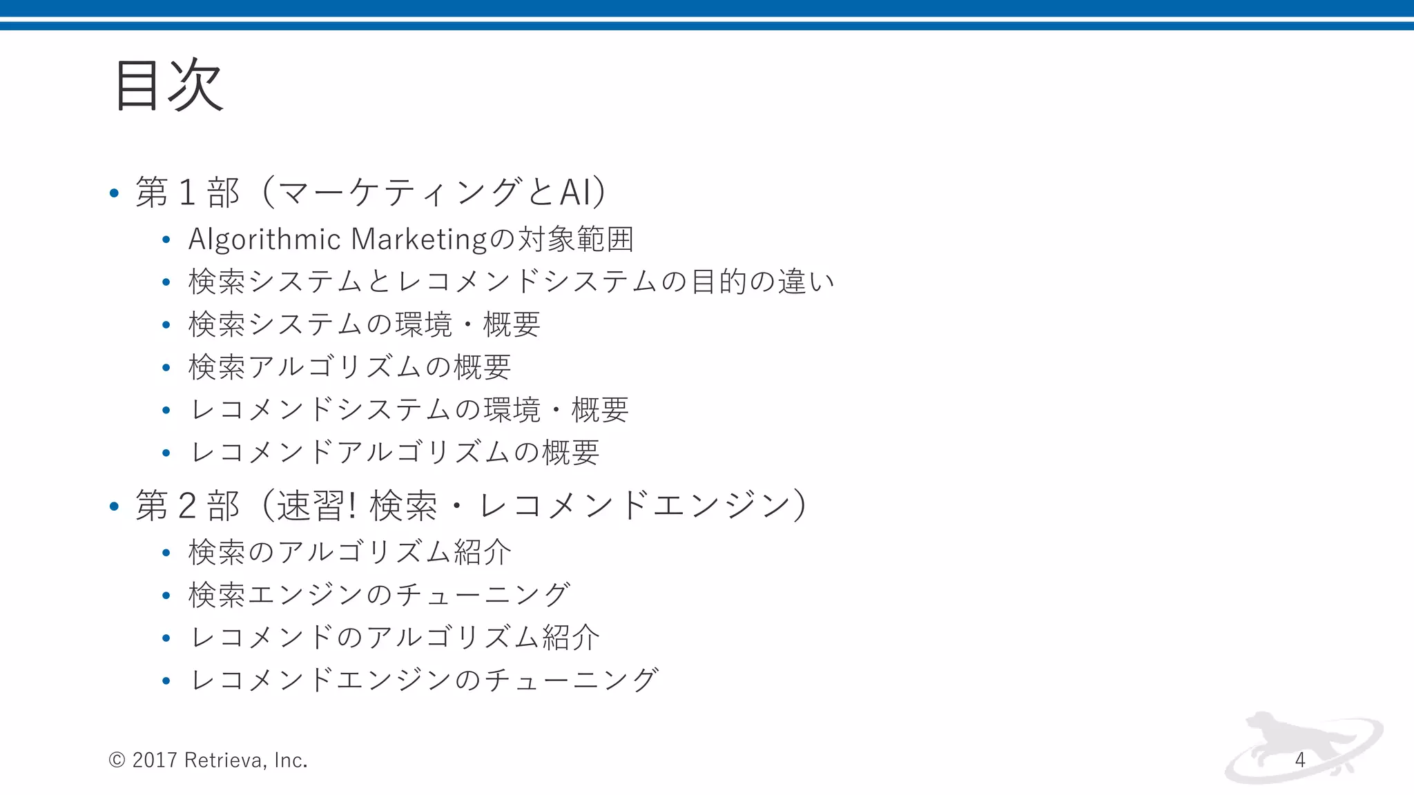
目次 • 第1部(マーケティングとAI) • Algorithmic
Marketingの対象範囲 • 検索システムとレコメンドシステムの目的の違い • 検索システムの環境・概要 • 検索アルゴリズムの概要 • レコメンドシステムの環境・概要 • レコメンドアルゴリズムの概要 • 第2部(速習! 検索・レコメンドエンジン) • 検索のアルゴリズム紹介 • 検索エンジンのチューニング • レコメンドのアルゴリズム紹介 • レコメンドエンジンのチューニング © 2017 Retrieva, Inc. 4
5.
お断り • 本書は主に、EC環境について記載されています。 © 2017
Retrieva, Inc. 5
6.
検索エンジンのアルゴリズム紹介 © 2017 Retrieva,
Inc. 6
7.
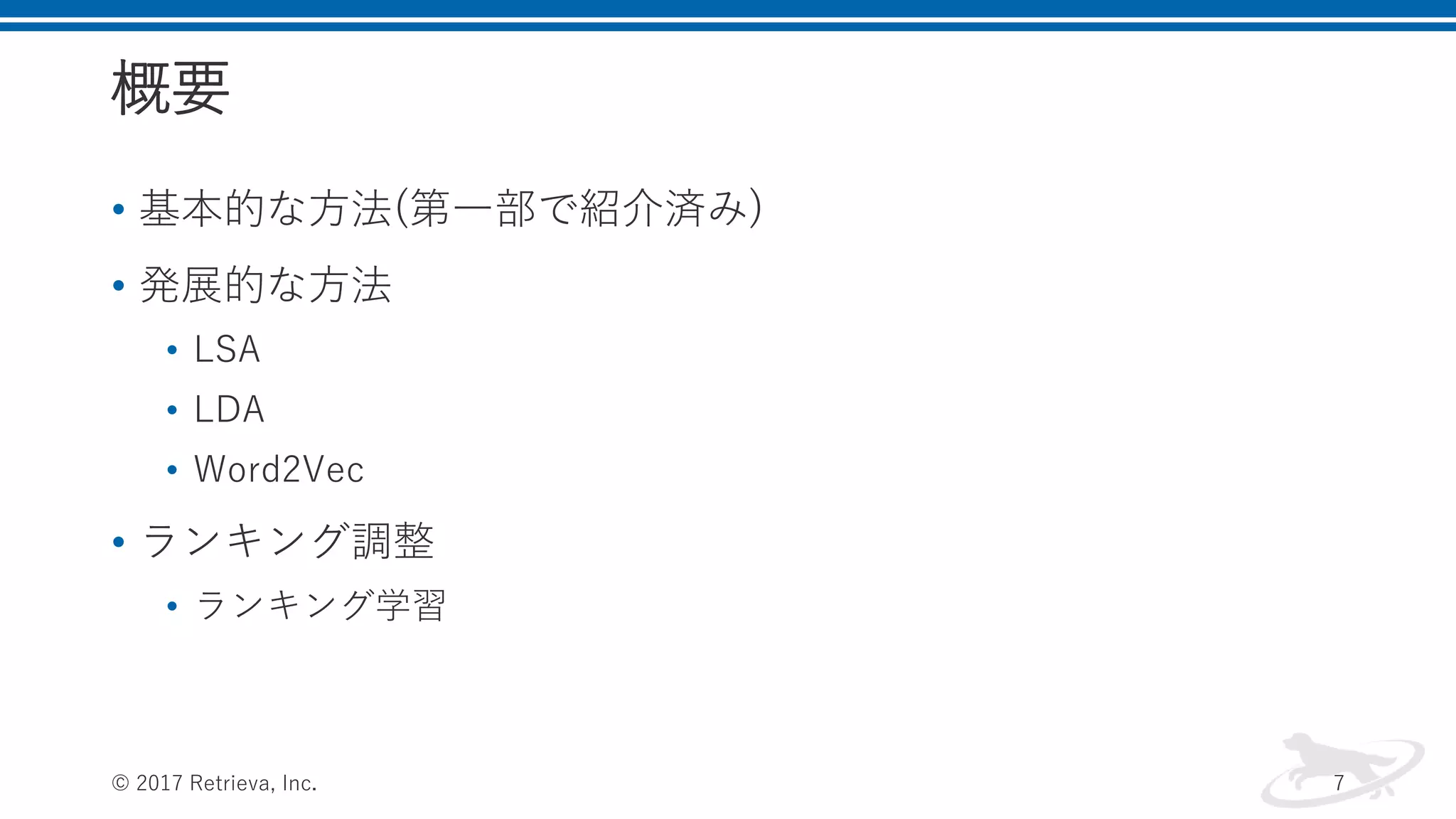
概要 • 基本的な方法(第一部で紹介済み) • 発展的な方法 •
LSA • LDA • Word2Vec • ランキング調整 • ランキング学習 © 2017 Retrieva, Inc. 7
8.
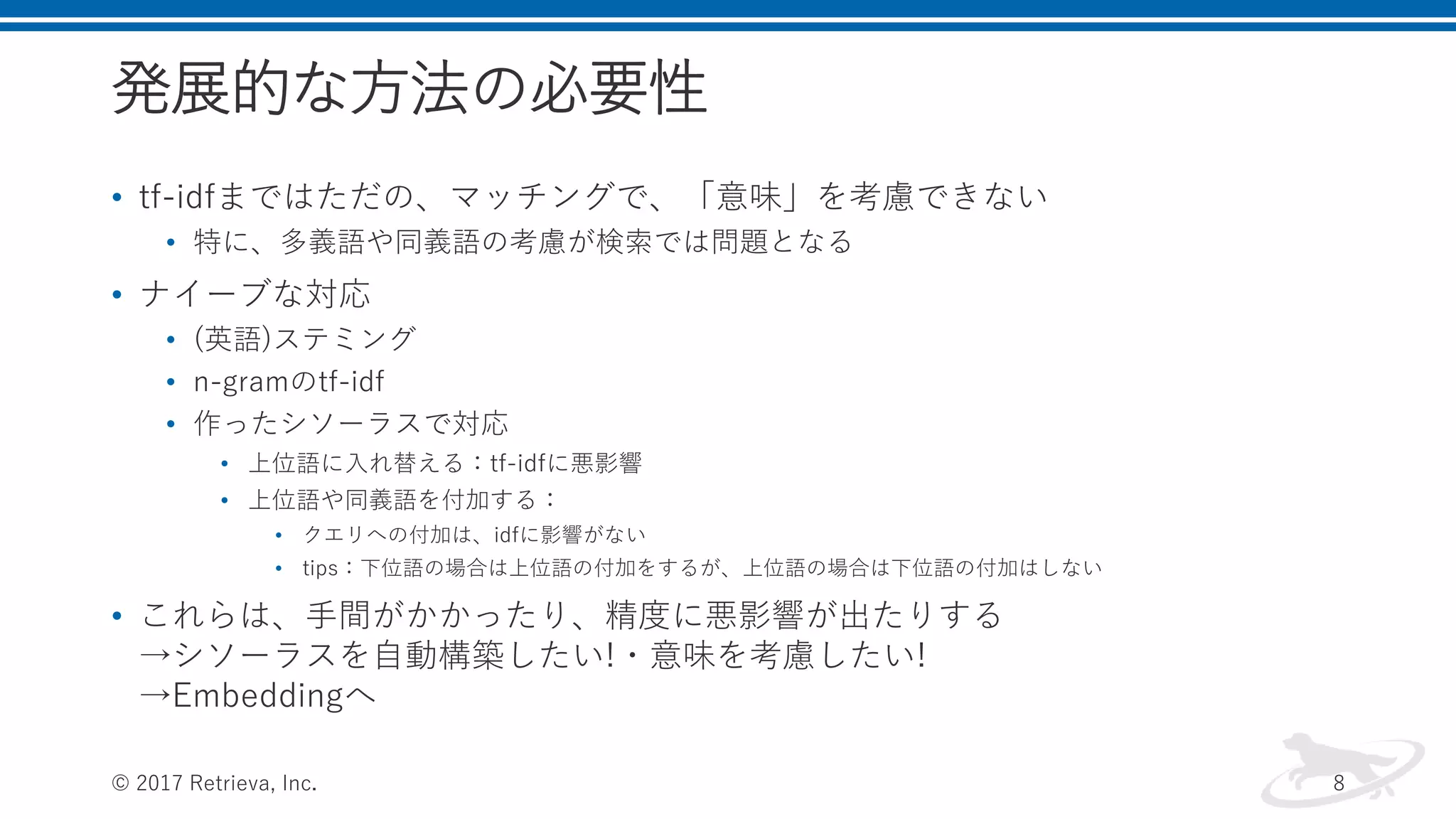
発展的な方法の必要性 • tf-idfまではただの、マッチングで、「意味」を考慮できない • 特に、多義語や同義語の考慮が検索では問題となる •
ナイーブな対応 • (英語)ステミング • n-gramのtf-idf • 作ったシソーラスで対応 • 上位語に入れ替える:tf-idfに悪影響 • 上位語や同義語を付加する: • クエリへの付加は、idfに影響がない • tips:下位語の場合は上位語の付加をするが、上位語の場合は下位語の付加はしない • これらは、手間がかかったり、精度に悪影響が出たりする →シソーラスを自動構築したい!・意味を考慮したい! →Embeddingへ © 2017 Retrieva, Inc. 8
9.
発展的な方法 • Embedding:単語を表現するベクトルを、連続値で表現する • 今まで:𝒗
𝒕 = [0,0, . . , 0,1,0, … , 0] • Embedding: 𝒗 𝒕 = [0.3,0.2, … , −0.04] • 連続値のベクトルで表現することの効果 • クエリに出現していないへの近さも考慮できる • その結果、精度が悪くなる場合も • クエリに入っていても、意味的に遠い単語は除外できる • Embeddingの精度とその後の計算方法が合っていれば • そのままクエリに使える • Embeddingの作成方法→LSA、pLSA、LDA、Word2Vec © 2017 Retrieva, Inc. 9
10.
LSA(Latent Semantic Analysis) •
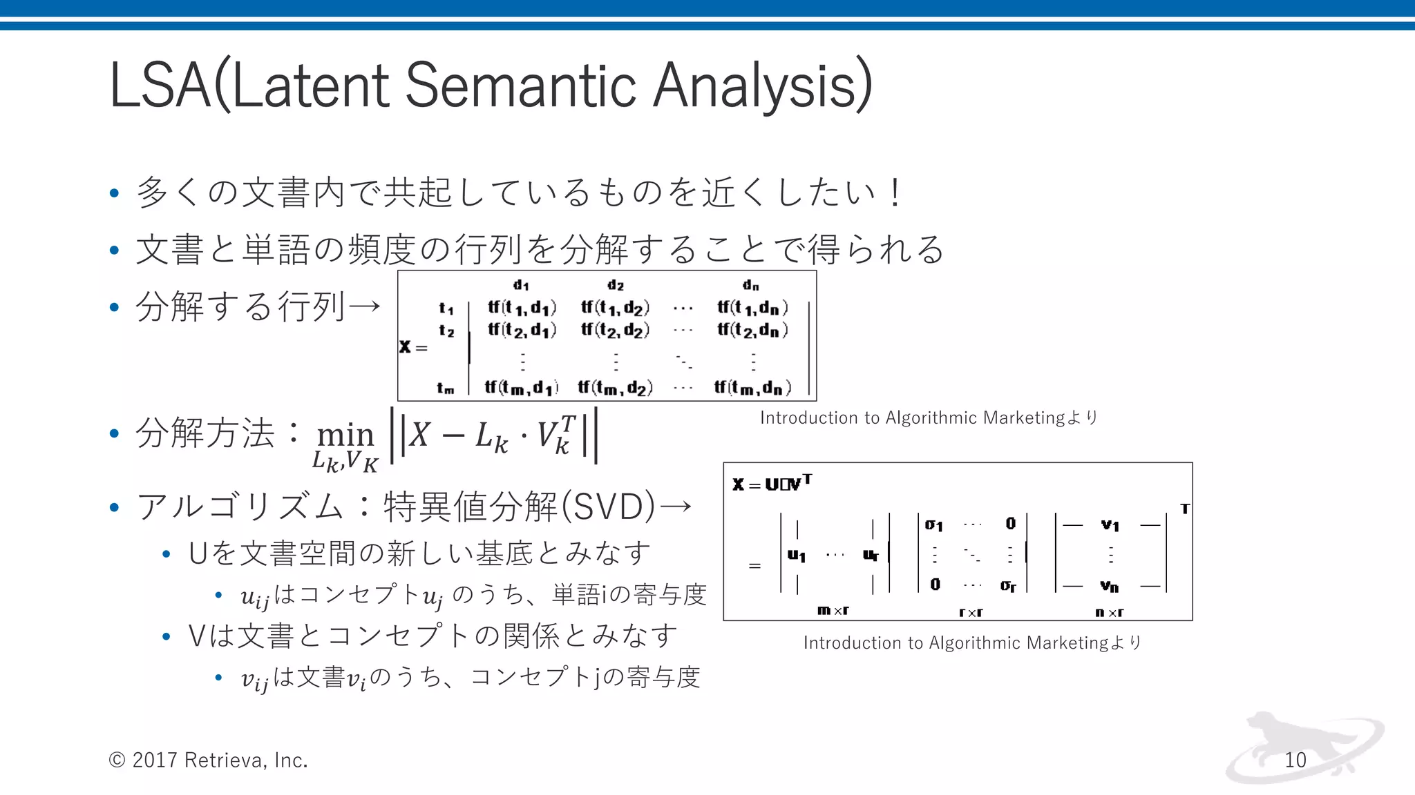
多くの文書内で共起しているものを近くしたい! • 文書と単語の頻度の行列を分解することで得られる • 分解する行列→ • 分解方法:min 𝐿 𝑘,𝑉 𝐾 𝑋 − 𝐿 𝑘 ⋅ 𝑉𝑘 𝑇 • アルゴリズム:特異値分解(SVD)→ • Uを文書空間の新しい基底とみなす • 𝑢𝑖𝑗はコンセプト𝑢𝑗 のうち、単語iの寄与度 • Vは文書とコンセプトの関係とみなす • 𝑣𝑖𝑗は文書𝑣𝑖のうち、コンセプトjの寄与度 © 2017 Retrieva, Inc. 10 Introduction to Algorithmic Marketingより Introduction to Algorithmic Marketingより
11.
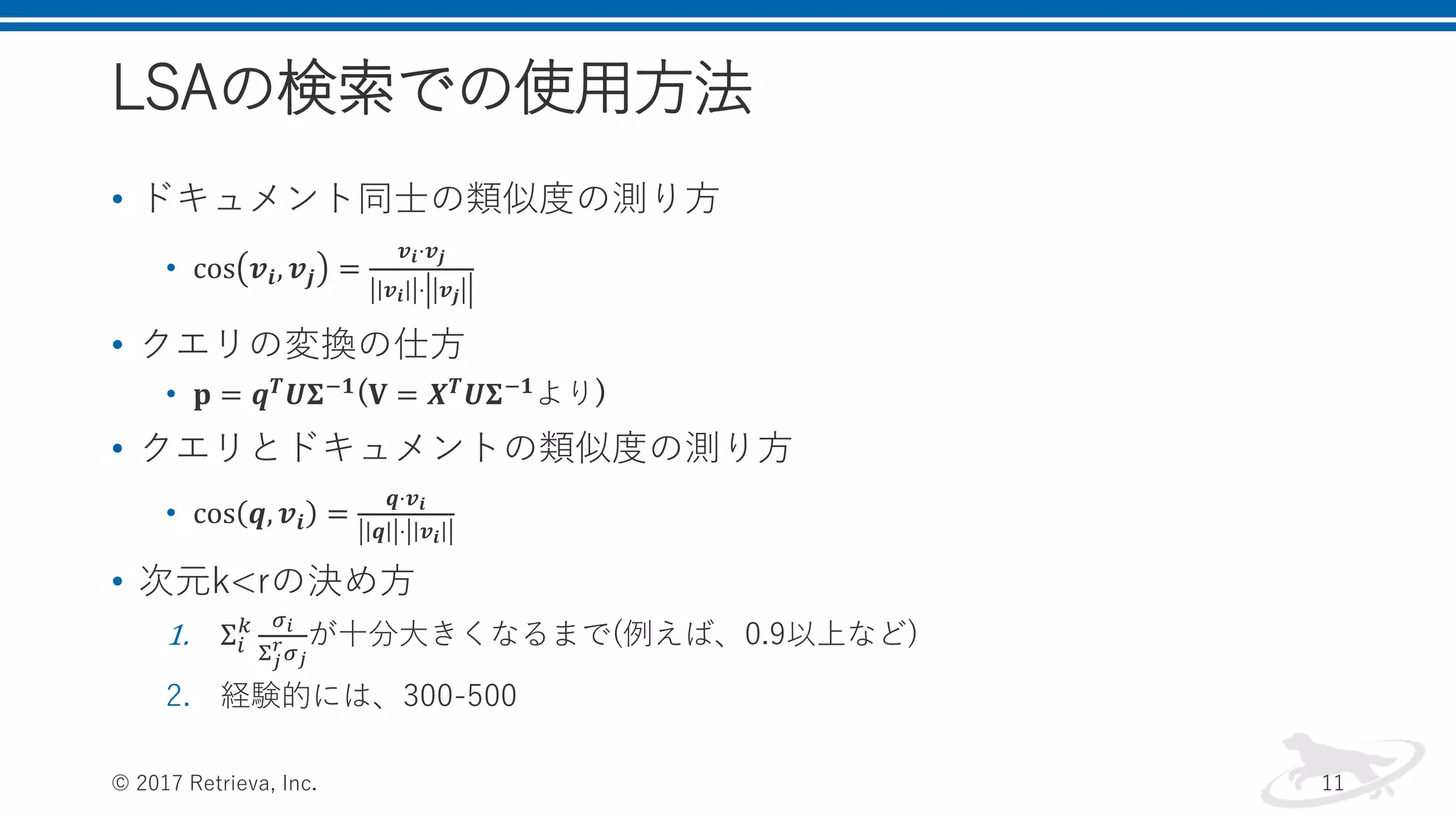
LSAの検索での使用方法 • ドキュメント同士の類似度の測り方 • cos
𝒗𝒊, 𝒗𝒋 = 𝒗 𝒊⋅𝒗 𝒋 𝒗 𝒊 ⋅ 𝒗 𝒋 • クエリの変換の仕方 • 𝐩 = 𝒒 𝑻 𝑼𝚺−𝟏 (𝐕 = 𝑿 𝑻 𝑼𝚺−𝟏 より) • クエリとドキュメントの類似度の測り方 • cos 𝒒, 𝒗𝒊 = 𝒒⋅𝒗 𝒊 𝒒 ⋅ 𝒗𝒊 • 次元k<rの決め方 1. Σ𝑖 𝑘 𝜎 𝑖 Σ 𝑗 𝑟 𝜎 𝑗 が十分大きくなるまで(例えば、0.9以上など) 2. 経験的には、300-500 © 2017 Retrieva, Inc. 11
12.
LSAの利点・問題点 • 利点 • 低次元空間で表現することで、同義語を考慮できる •
ノイズに強くなる • 再現率が高くなる • 自動的にembeddingが作れる • 問題点 • 多義語には難点がある(文書中の出現単語で考慮するため) • 前提としてる文書と単語のモデルがないので、どこまでできるかよくわからない • ベクトルの値が何を意味しているのかよくわからない • カウントデータなのに、ガウシアンを仮定している(負の値が取れてしまう) © 2017 Retrieva, Inc. 12
13.
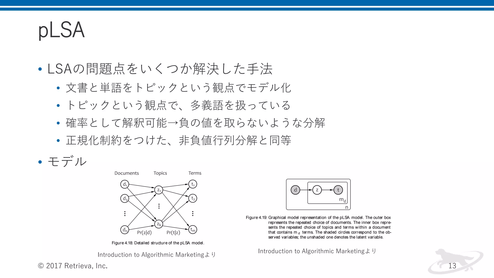
pLSA • LSAの問題点をいくつか解決した手法 • 文書と単語をトピックという観点でモデル化 •
トピックという観点で、多義語を扱っている • 確率として解釈可能→負の値を取らないような分解 • 正規化制約をつけた、非負値行列分解と同等 • モデル © 2017 Retrieva, Inc. 13 234 sear ch Figure 4.18: Detailed structure of the pLSA model. 234 sear ch Figure 4.18: Detailed structure of the pLSA model. Figure 4.19: Graphical model representation of the pLSA model. The outer box represents the repeated choice of documents. The inner box repre- sents the repeated choice of topics and terms within a document that contains m d terms. The shaded circles correspond to the ob- served variables; the unshaded one denotes the latent variable. Similarly to LSA, the pLSA model considers each document as a bag of words. From the probabilistic perspective, this means that the document–term pairs d,t are conditionally independent: Pr D,T Pr d,t (4.55) Introduction to Algorithmic Marketingより Introduction to Algorithmic Marketingより
14.
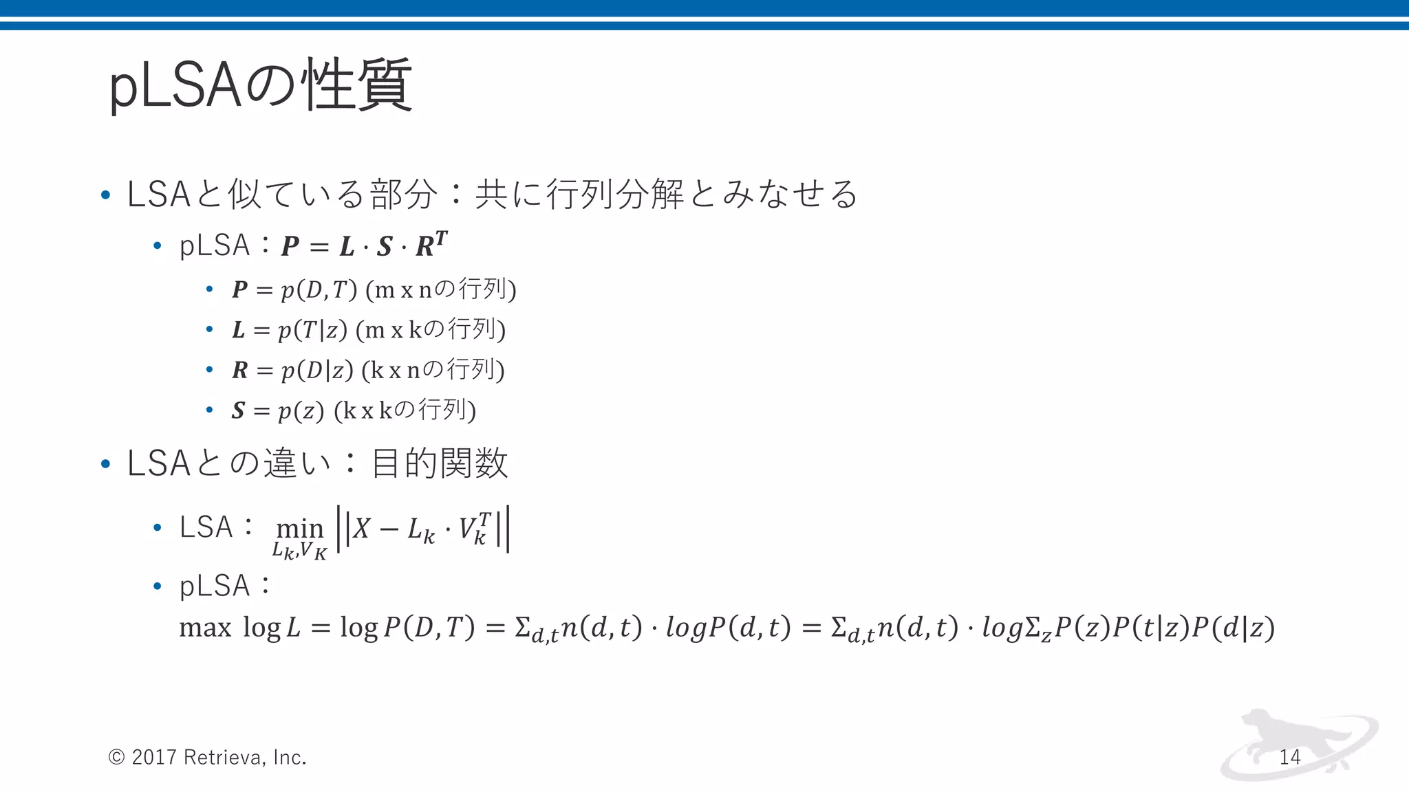
pLSAの性質 • LSAと似ている部分:共に行列分解とみなせる • pLSA:𝑷
= 𝑳 ⋅ 𝑺 ⋅ 𝑹 𝑻 • 𝑷 = 𝑝 𝐷, 𝑇 (m x nの行列) • 𝑳 = 𝑝 𝑇 𝑧 (m x kの行列) • 𝑹 = 𝑝 𝐷 𝑧 (k x nの行列) • 𝑺 = 𝑝(𝑧) (k x kの行列) • LSAとの違い:目的関数 • LSA: min 𝐿 𝑘,𝑉 𝐾 𝑋 − 𝐿 𝑘 ⋅ 𝑉𝑘 𝑇 • pLSA: max log 𝐿 = log 𝑃 𝐷, 𝑇 = Σ 𝑑,𝑡 𝑛 𝑑, 𝑡 ⋅ 𝑙𝑜𝑔𝑃 𝑑, 𝑡 = Σ 𝑑,𝑡 𝑛 𝑑, 𝑡 ⋅ 𝑙𝑜𝑔Σ 𝑧 𝑃 𝑧 𝑃 𝑡 𝑧 𝑃(𝑑|𝑧) © 2017 Retrieva, Inc. 14
15.
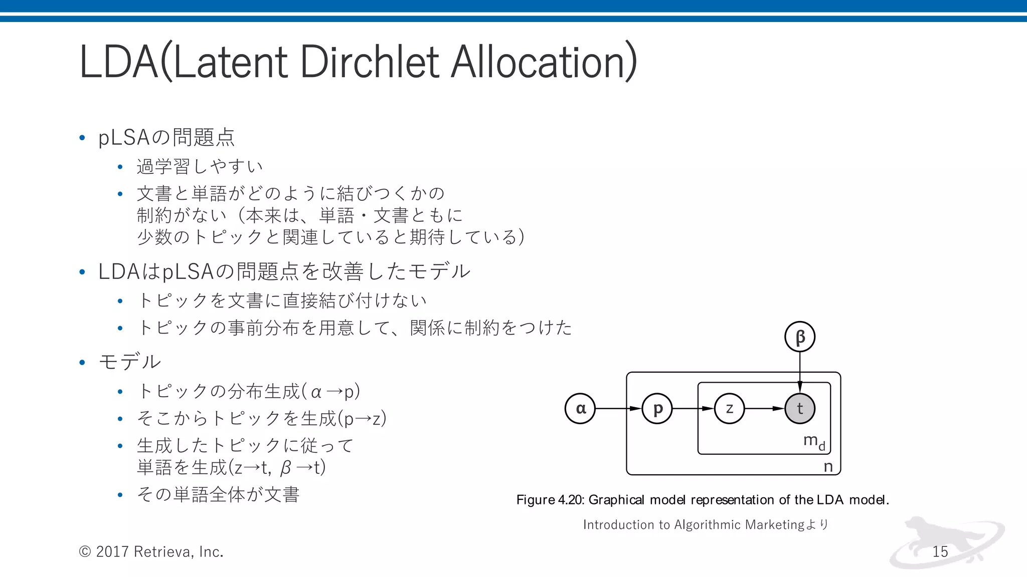
LDA(Latent Dirchlet Allocation) •
pLSAの問題点 • 過学習しやすい • 文書と単語がどのように結びつくかの 制約がない(本来は、単語・文書ともに 少数のトピックと関連していると期待している) • LDAはpLSAの問題点を改善したモデル • トピックを文書に直接結び付けない • トピックの事前分布を用意して、関係に制約をつけた • モデル • トピックの分布生成(α→p) • そこからトピックを生成(p→z) • 生成したトピックに従って 単語を生成(z→t, β→t) • その単語全体が文書 © 2017 Retrieva, Inc. 15 3.2. Choose a term t from the multinomial probability distribu- tion Pr t zt ;β conditioned on the topic zt . This distribu- tion is defined as the model parameter β for each pair of term and topic. In comparison with the pLSA process described in section 4.5.5.1, the key difference is that the LDA model draws topics from a global parametric distribution, not from the distributions learned for each doc- ument. The parameters of this model are the k-dimensional Dirichlet parameter ↵ and the k m matrix of term probabilities β, in which m is the total number of distinct terms in all documents. Each row of the matrix β defines the multinomial distributions over the words for a corresponding topic. These parameters are sampled once for a col- lection of documents, and, consequently, the number of parameters is smaller than that with pLSA. The graphical model that corresponds to the generative process is shown in Figure 4.20. Figure 4.20: Graphical model representation of the LDA model. In the context of a single document, the joint distribution of a topic mixture, all topics, and all terms is given by: Introduction to Algorithmic Marketingより
16.
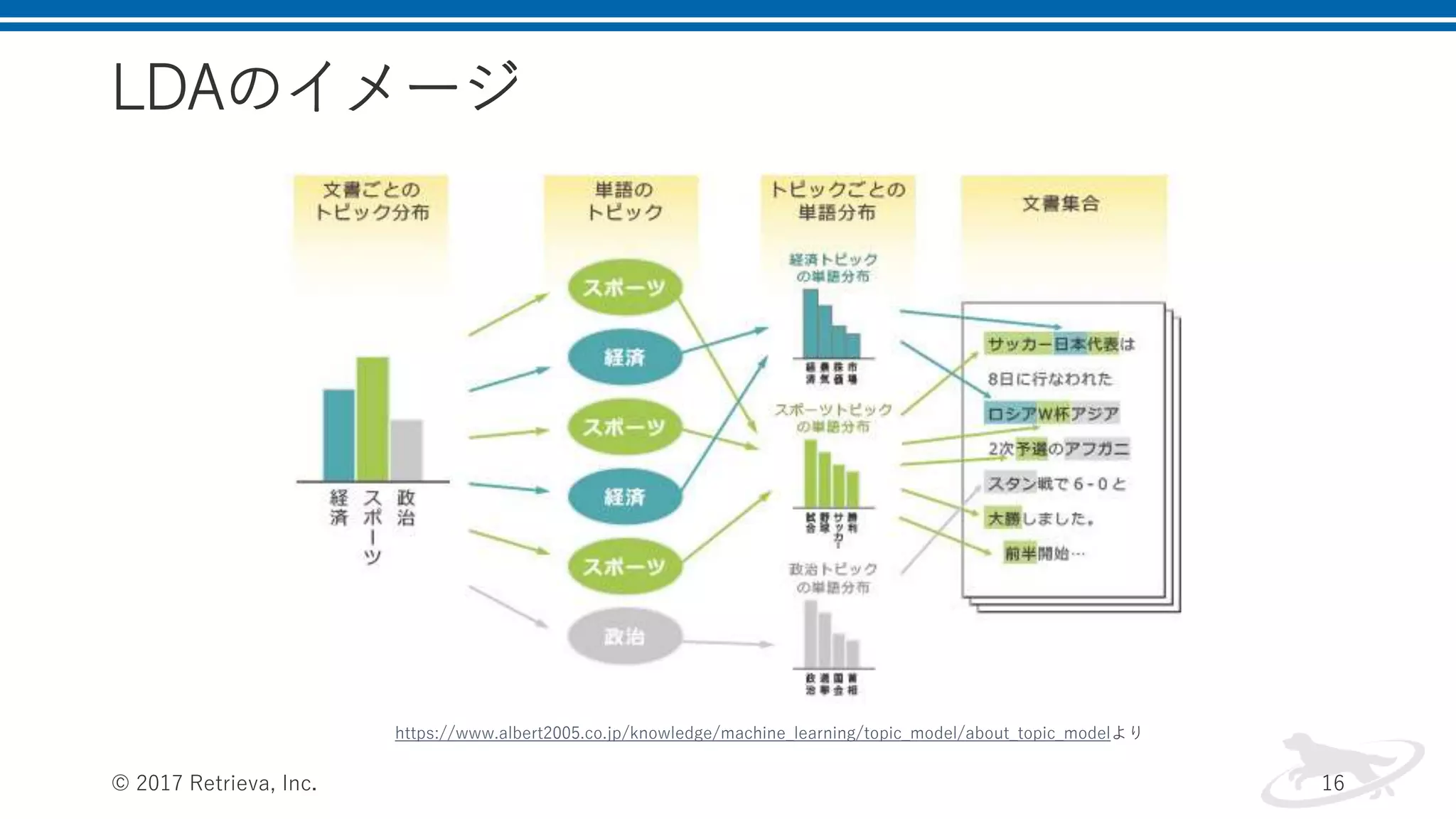
LDAのイメージ © 2017 Retrieva,
Inc. 16 https://www.albert2005.co.jp/knowledge/machine_learning/topic_model/about_topic_modelより
17.
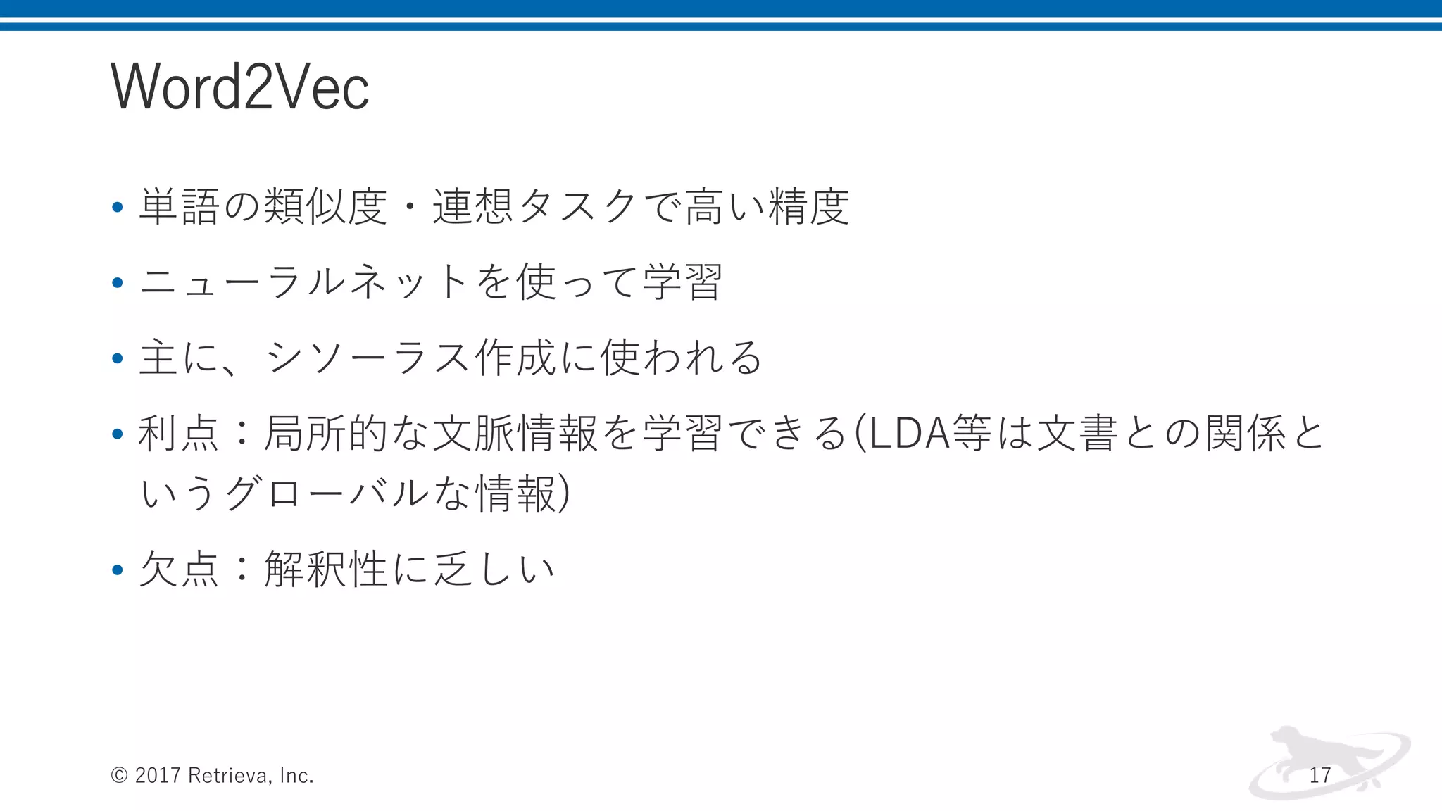
Word2Vec • 単語の類似度・連想タスクで高い精度 • ニューラルネットを使って学習 •
主に、シソーラス作成に使われる • 利点:局所的な文脈情報を学習できる(LDA等は文書との関係と いうグローバルな情報) • 欠点:解釈性に乏しい © 2017 Retrieva, Inc. 17
18.
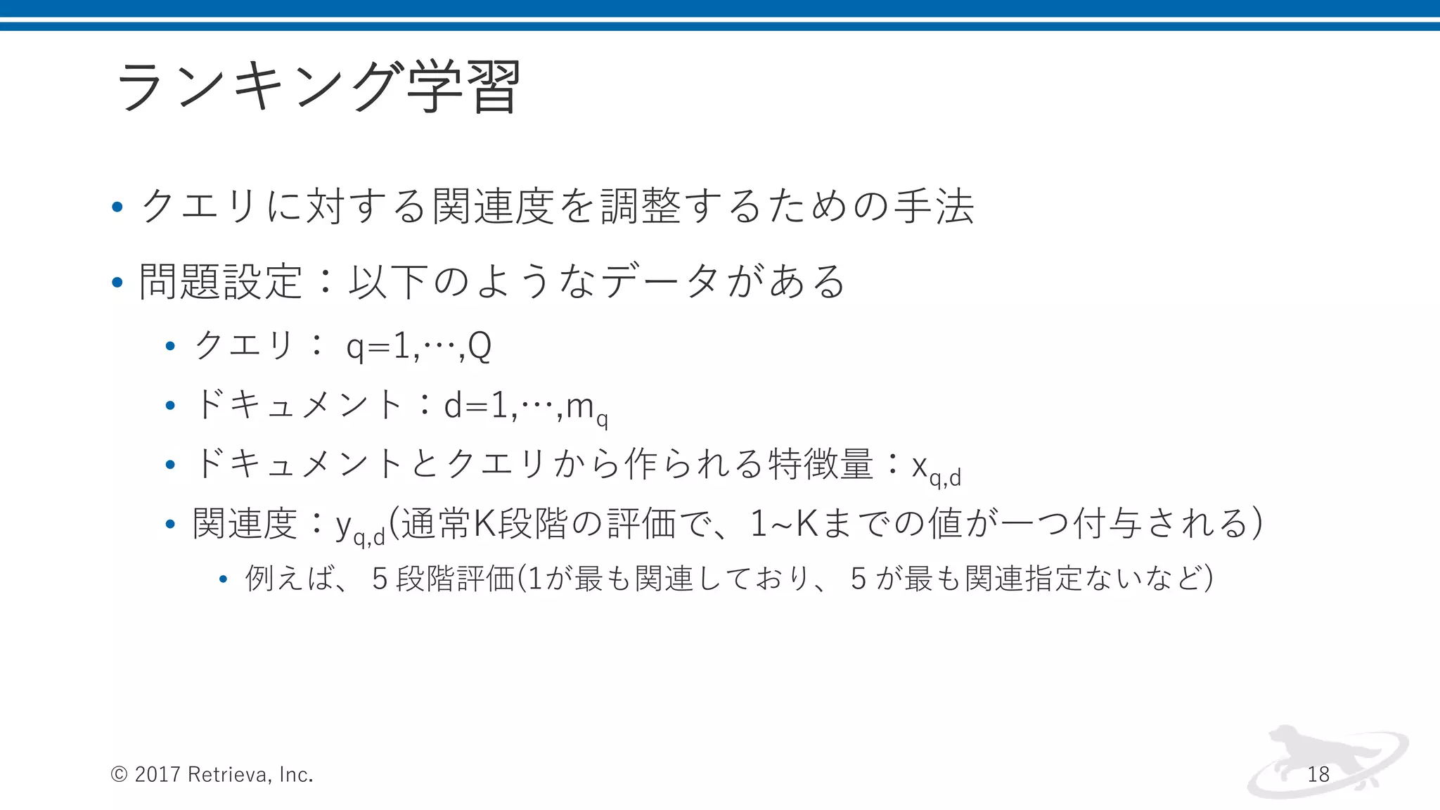
ランキング学習 • クエリに対する関連度を調整するための手法 • 問題設定:以下のようなデータがある •
クエリ: q=1,…,Q • ドキュメント:d=1,…,mq • ドキュメントとクエリから作られる特徴量:xq,d • 関連度:yq,d(通常K段階の評価で、1~Kまでの値が一つ付与される) • 例えば、5段階評価(1が最も関連しており、5が最も関連指定ないなど) © 2017 Retrieva, Inc. 18
19.
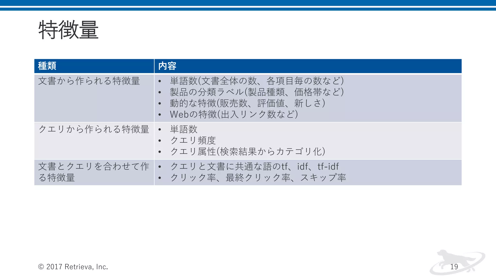
特徴量 種類 内容 文書から作られる特徴量 •
単語数(文書全体の数、各項目毎の数など) • 製品の分類ラベル(製品種類、価格帯など) • 動的な特徴(販売数、評価値、新しさ) • Webの特徴(出入リンク数など) クエリから作られる特徴量 • 単語数 • クエリ頻度 • クエリ属性(検索結果からカテゴリ化) 文書とクエリを合わせて作 る特徴量 • クエリと文書に共通な語のtf、idf、tf-idf • クリック率、最終クリック率、スキップ率 © 2017 Retrieva, Inc. 19
20.
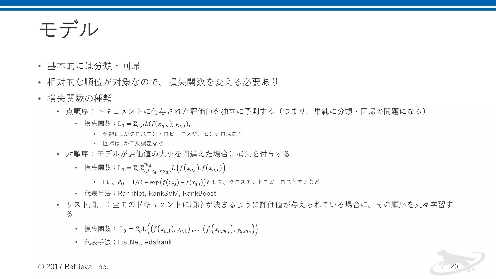
モデル • 基本的には分類・回帰 • 相対的な順位が対象なので、損失関数を変える必要あり •
損失関数の種類 • 点順序:ドキュメントに付与された評価値を独立に予測する(つまり、単純に分類・回帰の問題になる) • 損失関数:L0 = Σ 𝑞,𝑑 𝐿(𝑓 𝑥 𝑞,𝑑 , 𝑦 𝑞,𝑑), • 分類はLがクロスエントロピーロスや、ヒンジロスなど • 回帰はLが二乗誤差など • 対順序:モデルが評価値の大小を間違えた場合に損失を付与する • 損失関数:L0 = Σ 𝑞Σ𝑖,𝑗:𝑦 𝑞,𝑖>𝑦 𝑞,𝑗 𝑚 𝑞 𝐿 𝑓 𝑥 𝑞,𝑖 , 𝑓 𝑥 𝑞,𝑗 • Lは、𝑃𝑖𝑗 = 1/(1 + exp 𝑓 𝑥 𝑞,𝑖 − 𝑓 𝑥 𝑞,𝑗 として、クロスエントロピーロスとするなど • 代表手法:RankNet, RankSVM, RankBoost • リスト順序:全てのドキュメントに順序が決まるように評価値が与えられている場合に、その順序を丸々学習す る • 損失関数: L0 = Σ 𝑞L 𝑓 𝑥 𝑞,1 , 𝑦 𝑞,1 , … , 𝑓 𝑥 𝑞,𝑚 𝑞 , 𝑦𝑞,𝑚 𝑞 • 代表手法:ListNet, AdaRank © 2017 Retrieva, Inc. 20
21.
ラベルづけ • 通常は専門家などが行う。これには多大な労力が伴い、動的な チューニングができない • そのため、動的なチューニングはみなしのラベルづけをする必 要がある •
方法は主に3種類ある • 単クエリに対して • クエリチェーンに対して • クエリチェーン中の異なるドキュメントに対して © 2017 Retrieva, Inc. 21
22.
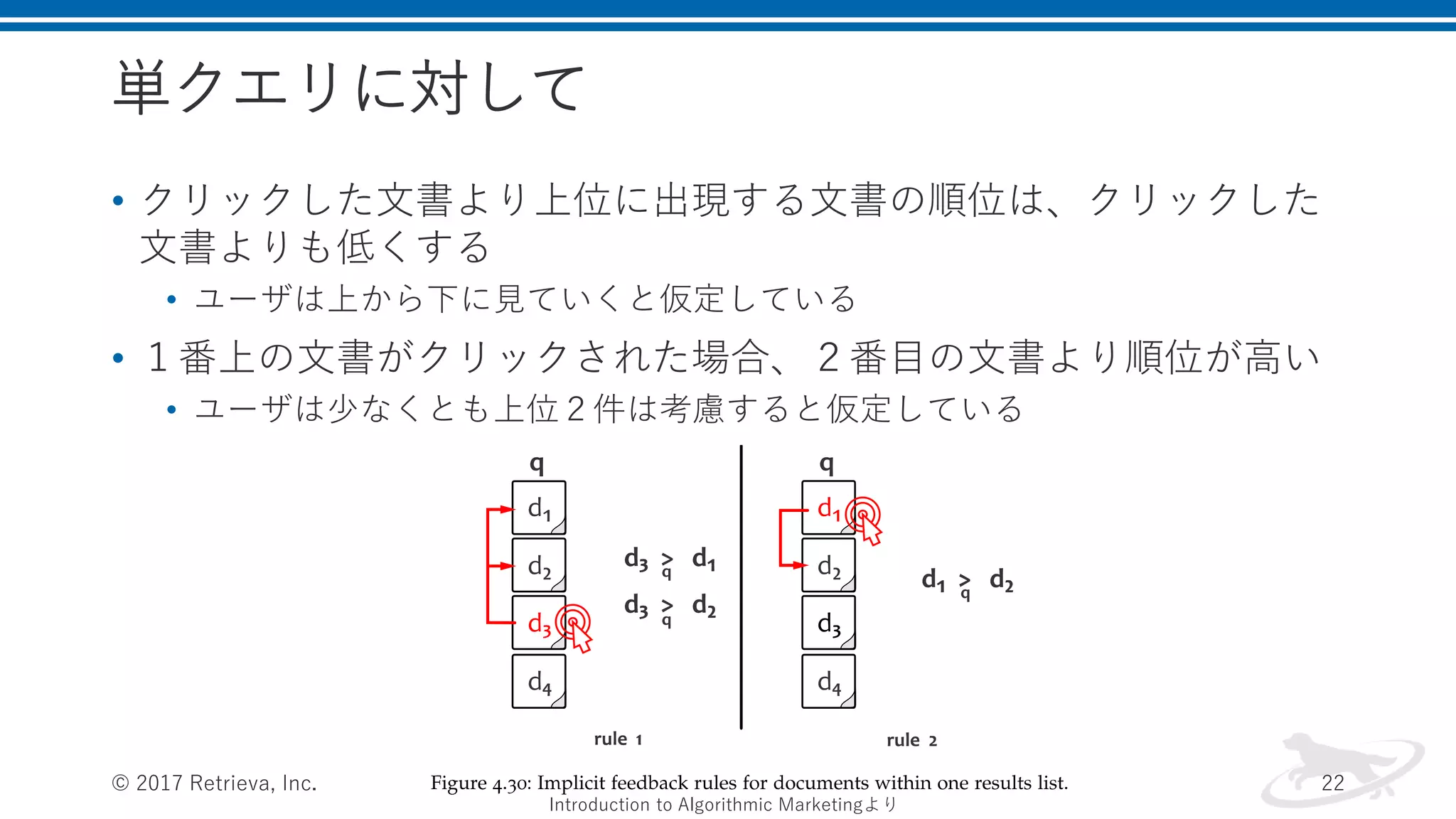
単クエリに対して • クリックした文書より上位に出現する文書の順位は、クリックした 文書よりも低くする • ユーザは上から下に見ていくと仮定している •
1番上の文書がクリックされた場合、2番目の文書より順位が高い • ユーザは少なくとも上位2件は考慮すると仮定している © 2017 Retrieva, Inc. 22 Introduction to Algorithmic Marketingより
23.
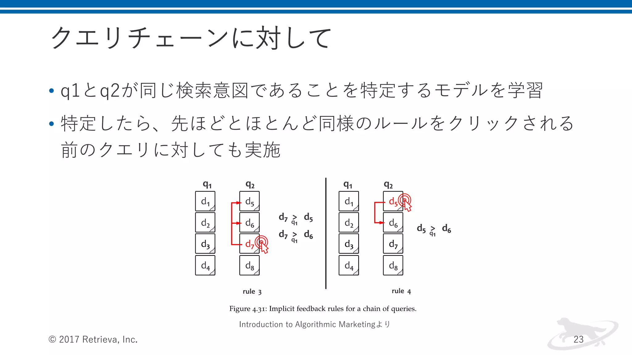
クエリチェーンに対して • q1とq2が同じ検索意図であることを特定するモデルを学習 • 特定したら、先ほどとほとんど同様のルールをクリックされる 前のクエリに対しても実施 ©
2017 Retrieva, Inc. 23 Introduction to Algorithmic Marketingより
24.
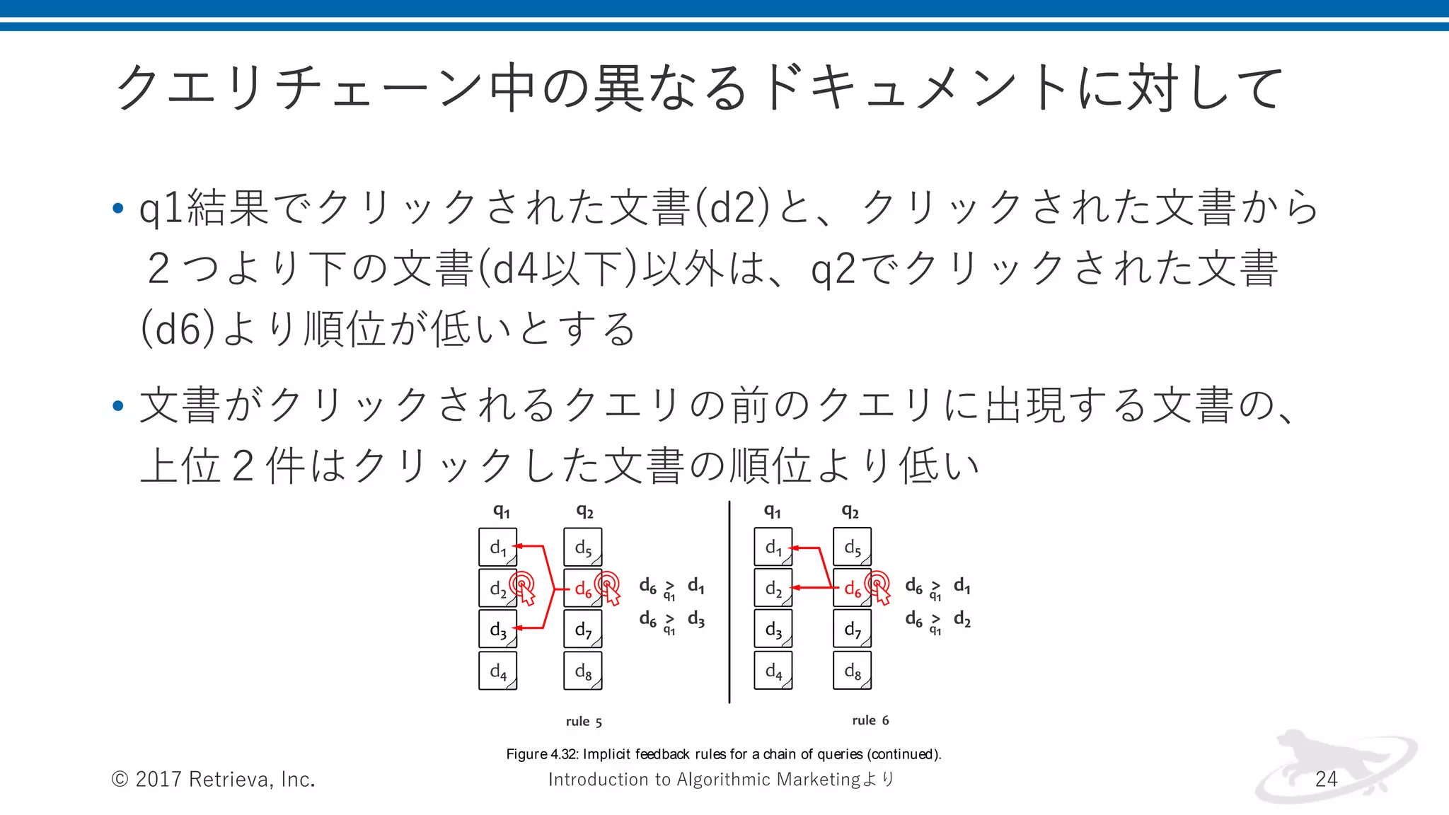
クエリチェーン中の異なるドキュメントに対して • q1結果でクリックされた文書(d2)と、クリックされた文書から 2つより下の文書(d4以下)以外は、q2でクリックされた文書 (d6)より順位が低いとする • 文書がクリックされるクエリの前のクエリに出現する文書の、 上位2件はクリックした文書の順位より低い ©
2017 Retrieva, Inc. 24 268 sear ch The last two rules are shown in Figure 4.32. These rules establish relevance relationships between the documents from different results lists in a query chain. Rule 5 states that documents that are viewed but not clicked on in the results list for query q1 are less relevant than the documents that are clicked on in the results set for query q2 . This relevance relationship is established with regard to the earlier query. Consistently with rules 1 and 2, documents are considered to be viewed if they are above the clicked ones or right below the last clicked document, like document d3 in Figure 4.32. Finally, rule 6 states that documents clicked on in the later results list are more relevant than the first two documents in the former list. This rule is based on the assumption that a user analyzes at least the first two results in the list before reformulating a query. Figure 4.32: Implicit feedback rules for a chain of queries (continued). All six rules are simultaneously evaluated against each query chain Introduction to Algorithmic Marketingより
25.
検索エンジンのチューニング © 2017 Retrieva,
Inc. 25
26.
概要 • 構造化データのチューニング • E-Commerceでの実践 ©
2017 Retrieva, Inc. 26
27.
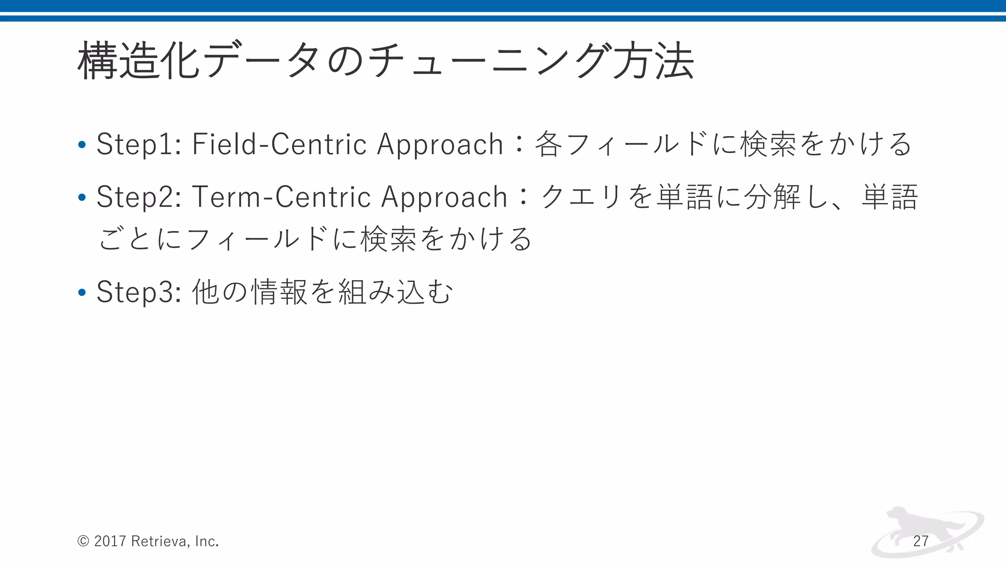
構造化データのチューニング方法 • Step1: Field-Centric
Approach:各フィールドに検索をかける • Step2: Term-Centric Approach:クエリを単語に分解し、単語 ごとにフィールドに検索をかける • Step3: 他の情報を組み込む © 2017 Retrieva, Inc. 27
28.
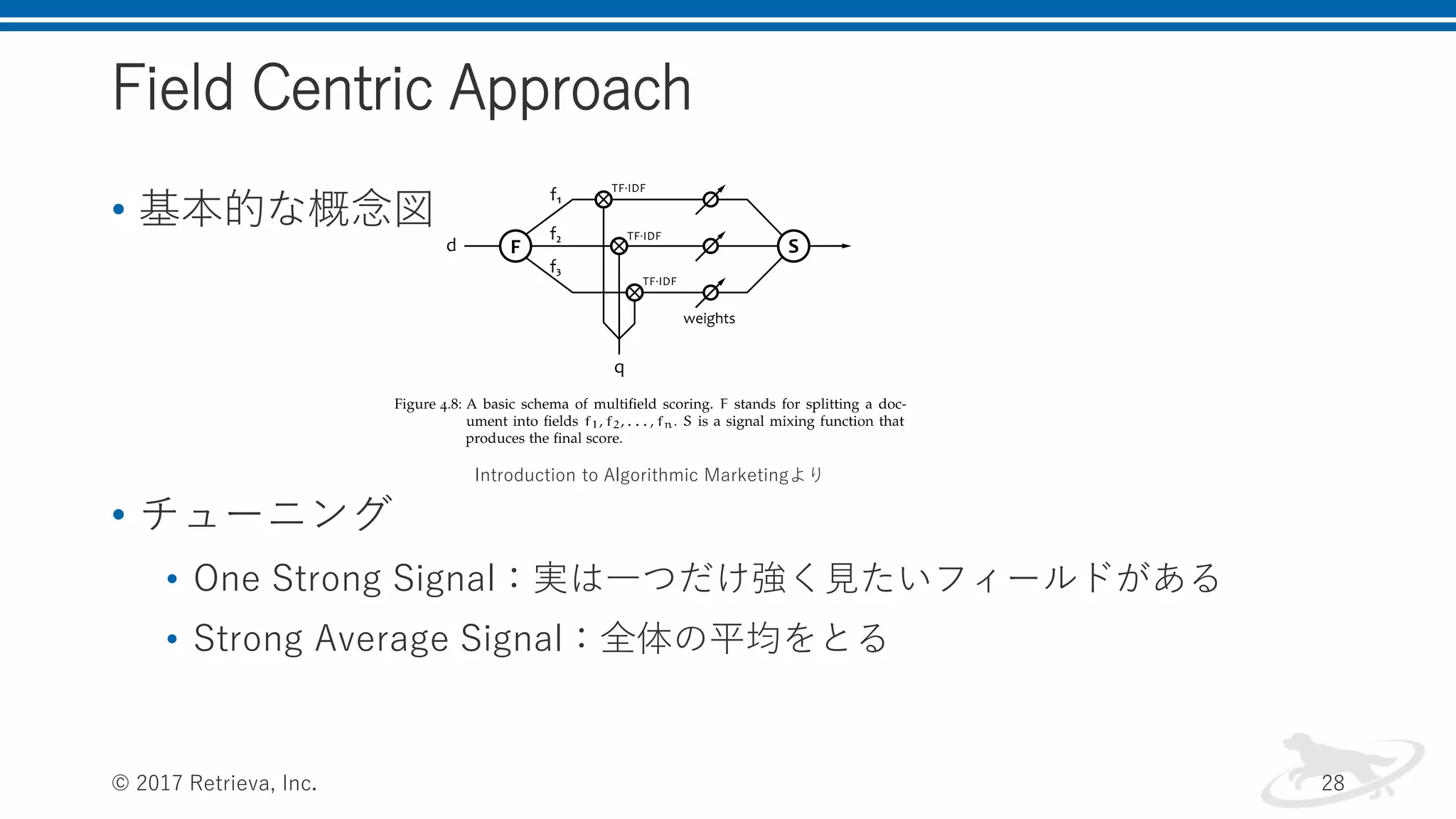
Field Centric Approach •
基本的な概念図 • チューニング • One Strong Signal:実は一つだけ強く見たいフィールドがある • Strong Average Signal:全体の平均をとる © 2017 Retrieva, Inc. 28 Introduction to Algorithmic Marketingより
29.
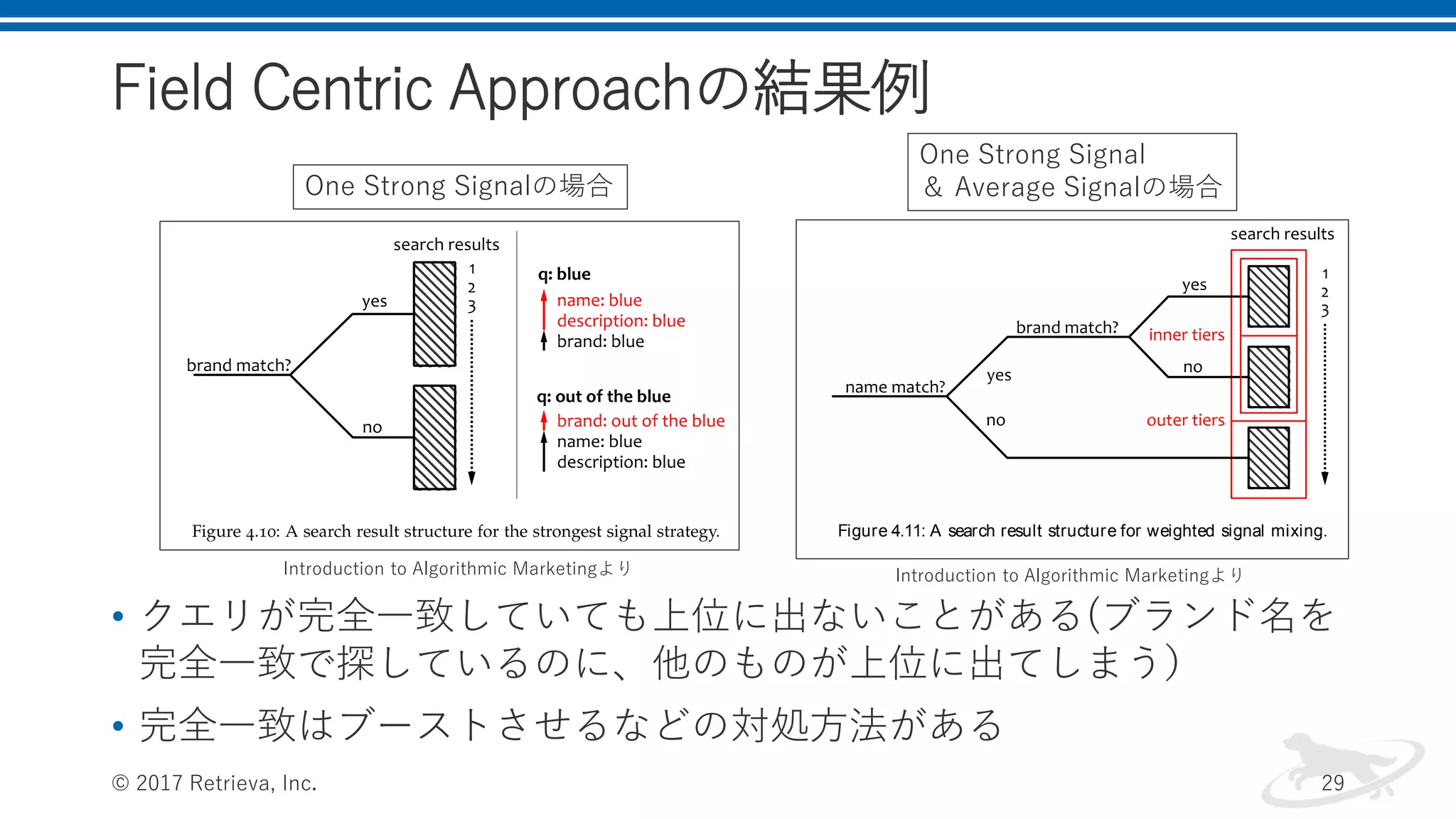
Field Centric Approachの結果例 •
クエリが完全一致していても上位に出ないことがある(ブランド名を 完全一致で探しているのに、他のものが上位に出てしまう) • 完全一致はブーストさせるなどの対処方法がある © 2017 Retrieva, Inc. 29 query, but we can also keep brand matching as a second priority, as il- lustrated in Figure 4.11. This can be implemented by using the scoring function 4.34 and setting weights such that the product name signal is amplified and the matching items are elevated to the top tier of the search results list. Brand matching will be the second-strongest signal in the mix, so the items in the inner tiers created by name matching will be ranked based on the brand. A signal mixing pipeline that im- plements this strategy is shown in Figure 4.12. Figure 4.11: A search result structure for weighted signal mixing. One Strong Signalの場合 One Strong Signal & Average Signalの場合 Introduction to Algorithmic Marketingより Introduction to Algorithmic Marketingより
30.
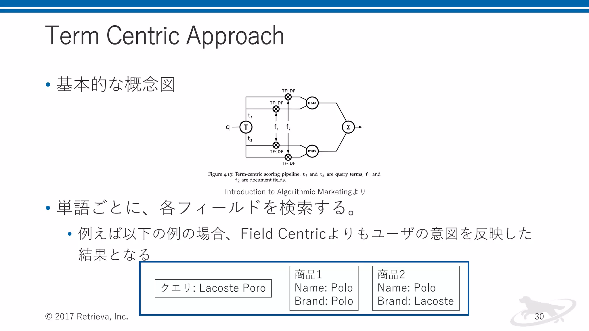
Term Centric Approach •
基本的な概念図 • 単語ごとに、各フィールドを検索する。 • 例えば以下の例の場合、Field Centricよりもユーザの意図を反映した 結果となる © 2017 Retrieva, Inc. 30 クエリ: Lacoste Poro 商品1 Name: Polo Brand: Polo 商品2 Name: Polo Brand: Lacoste Introduction to Algorithmic Marketingより
31.
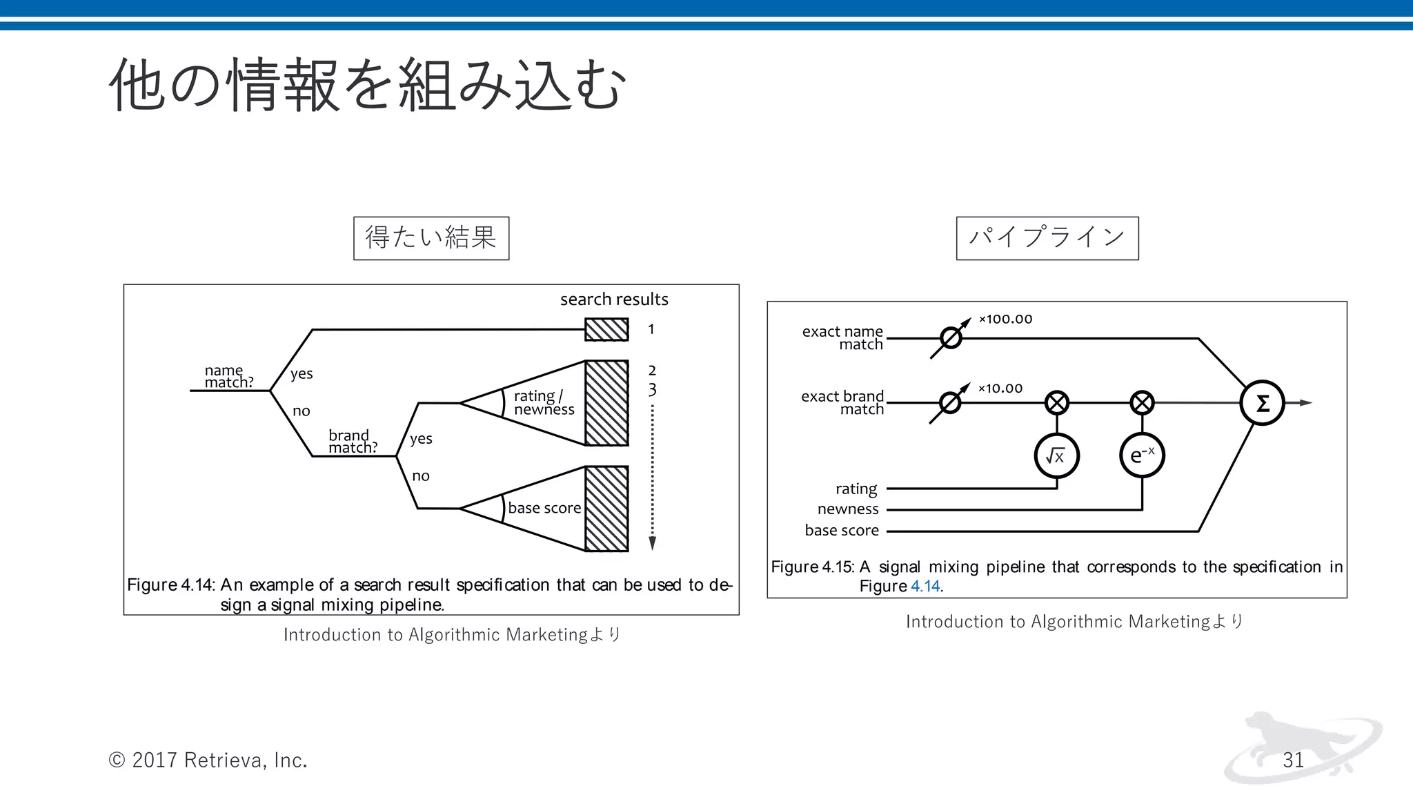
他の情報を組み込む © 2017 Retrieva,
Inc. 31 216 sear ch • Otherwise, the results should be ranked according to average relevance of product descriptions and other fields. Figure 4.14: An example of a search result specification that can be used to de- sign a signal mixing pipeline. The specification mentions five different signals that should be taken into account: exact product name or ID match, exact brand match, product newness, product rating, and base average score. The exact match signals can be obtained by using n-gram scoring for the cor- responding name and brand fields. A reasonably good precision can be implemented by using bigrams, and even stricter matching can be factor, and we also have to mix it with the rating and newness features to achieve the desired secondary sorting, as shown in Figure 4.15. We clearly need to rescale the raw rating and newness values to convert them into meaningful scoring factors; this can be done in many dif- ferent ways. A raw customer rating on a scale from 1 to 5 can be too aggressive as an amplification factor and can be tempered by using a square root or logarithm function to reduce the gap between low-rated and high-rated products. For instance, the magnitude of the brand sig- nal amplified by a raw rating of 5.0 is two times higher than for a rating of 2.5; however, by taking the square root of the rating, we reduce the difference down to 1.41. Figure 4.15: A signal mixing pipeline that corresponds to the specification in Figure 4.14. The newness value should be transformed into a factor that gradu- ally decreases with the age of a product. This can be done by using a linear function, exponential decay, or Gaussian decay. For example, it can be a reasonable choice to decrease the scoring factor by 10% every 30 days, which leads us to the exponential decay function newness factor exp ↵x (4.38) 得たい結果 パイプライン Introduction to Algorithmic Marketingより Introduction to Algorithmic Marketingより
32.
E-Commerceでの実践 © 2017 Retrieva,
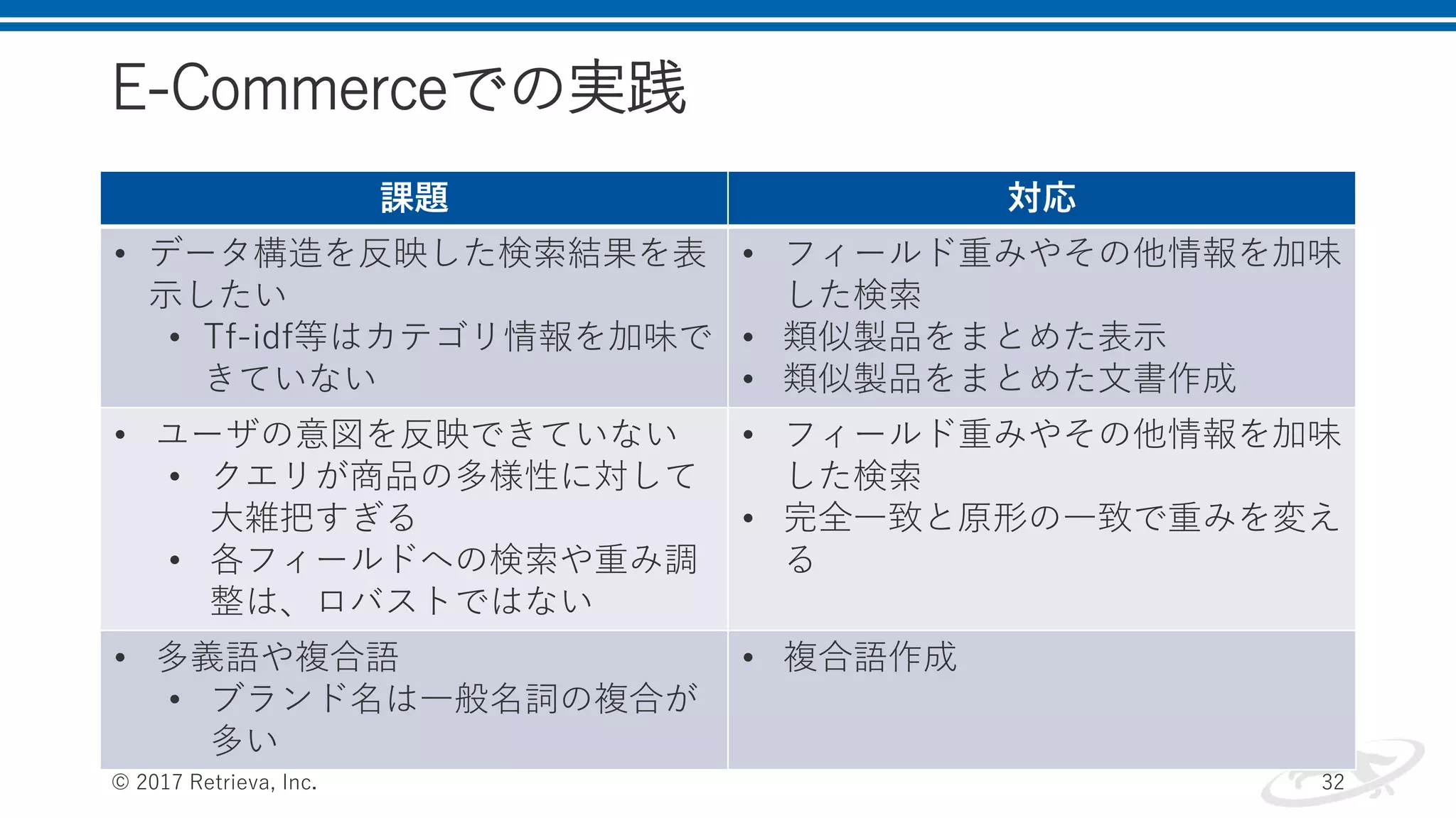
Inc. 32 課題 対応 • データ構造を反映した検索結果を表 示したい • Tf-idf等はカテゴリ情報を加味で きていない • フィールド重みやその他情報を加味 した検索 • 類似製品をまとめた表示 • 類似製品をまとめた文書作成 • ユーザの意図を反映できていない • クエリが商品の多様性に対して 大雑把すぎる • 各フィールドへの検索や重み調 整は、ロバストではない • フィールド重みやその他情報を加味 した検索 • 完全一致と原形の一致で重みを変え る • 多義語や複合語 • ブランド名は一般名詞の複合が 多い • 複合語作成
33.
E-Commerceでの実践 • 得られる示唆 • 適合率(Precision)が大事 •
完全一致が大事 • 単純なスコアリングより、属性構造の反映が大事 © 2017 Retrieva, Inc. 33
34.
レコメンドエンジンの アルゴリズム紹介 © 2017 Retrieva,
Inc. 34
35.
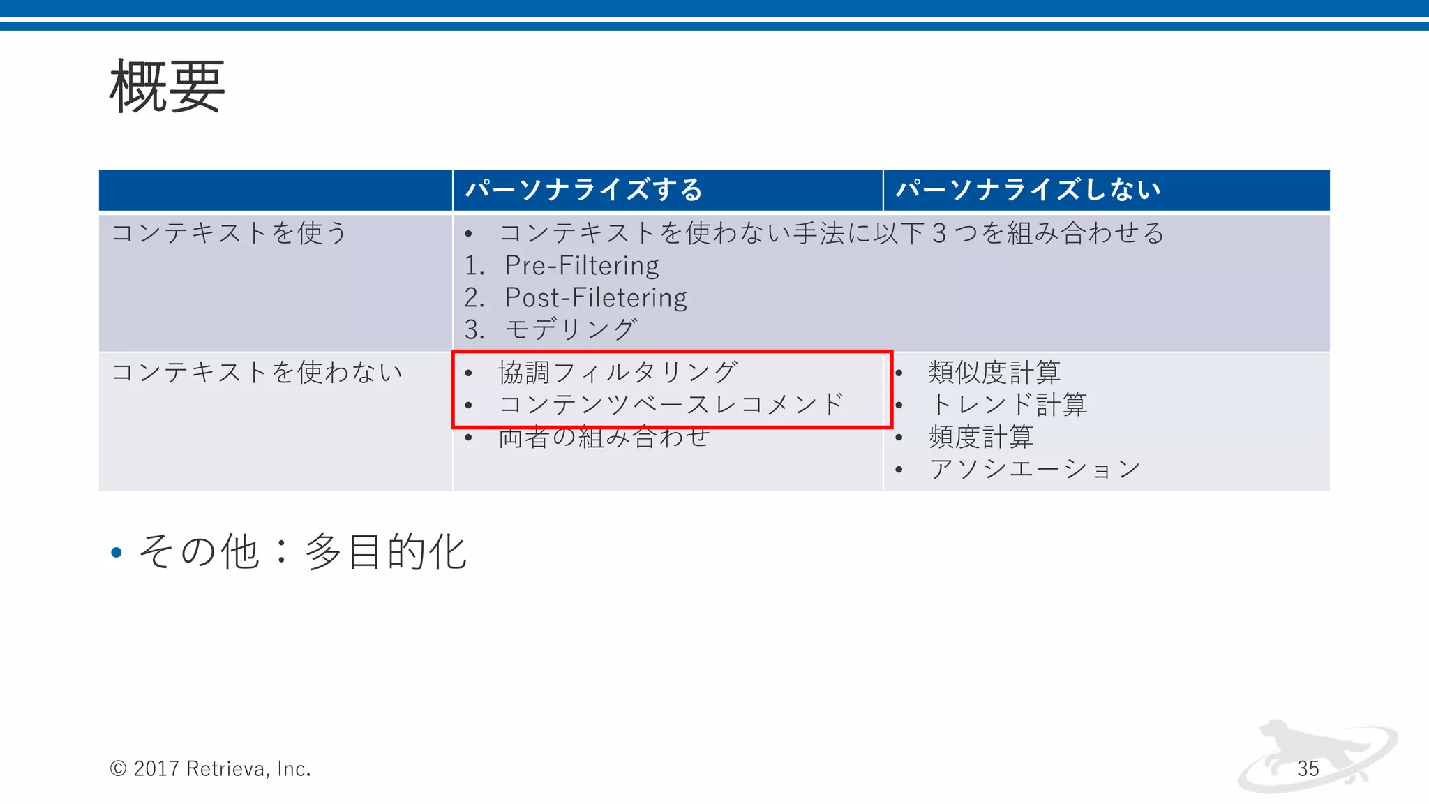
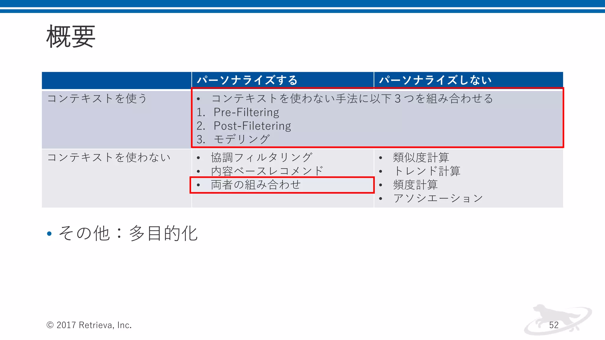
概要 • その他:多目的化 © 2017
Retrieva, Inc. 35 パーソナライズする パーソナライズしない コンテキストを使う • コンテキストを使わない手法に以下3つを組み合わせる 1. Pre-Filtering 2. Post-Filetering 3. モデリング コンテキストを使わない • 協調フィルタリング • コンテンツベースレコメンド • 両者の組み合わせ • 類似度計算 • トレンド計算 • 頻度計算 • アソシエーション
36.
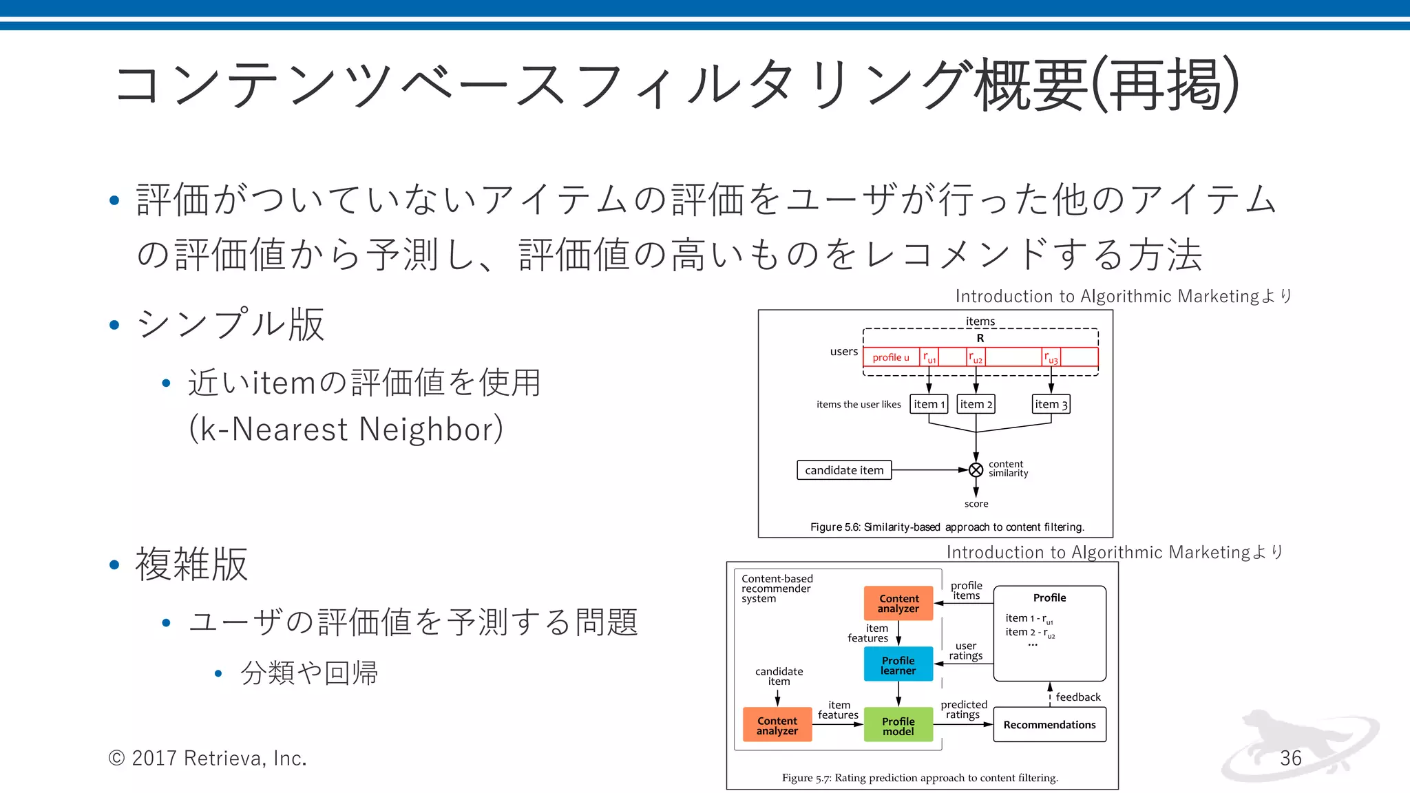
コンテンツベースフィルタリング概要(再掲) • 評価がついていないアイテムの評価をユーザが行った他のアイテム の評価値から予測し、評価値の高いものをレコメンドする方法 • シンプル版 •
近いitemの評価値を使用 (k-Nearest Neighbor) • 複雑版 • ユーザの評価値を予測する問題 • 分類や回帰 © 2017 Retrieva, Inc. 36 lies mainly on the catalog data (content) and uses only a small fraction of the information available in the rating matrix. This is the reason why this group of methods is referred to as content filtering. The main idea of content filtering is quite straightforward: take items that the user positively rated in the past and recommend other items similar to these examples, as shown in Figure 5.6. The important constraint, how- ever, is that the measure of similarity is based on the item content 1 and does not include behavioral data, such as information about items that are frequently purchased or rated together by other users. This effec- tively means that a content-based recommender system uses only one row of the rating matrix – the profile of the user for whom the recom- mendations are prepared. This limited usage of the rating information is typically counterbalanced by a similarity function that uses a wide range of carefully engineered item features. The recommendations are then ranked according to their similarity scores and, optionally, the rating values of corresponding items in the profile. For example, as- suming that item 1 has the highest rating in the example shown in Figure 5.6, that is, ru 1 ru 2 and ru 1 ru 3, a candidate item similar to item 1 can be ranked higher than candidate items equally similar to items 2 or 3. Figure 5.6: Similarity-based approach to content filtering. The above approach to content filtering is, however, somewhat lim- ited because it inherently relies on a nearest neighbor model for rating 1 See Chapter 4 for a detailed discussion of such measures. One of the most common exam- ples would be the TF IDF distance between textual descriptions discussed in Section 4.3.5. Introduction to Algorithmic Marketingより Introduction to Algorithmic Marketingより
37.
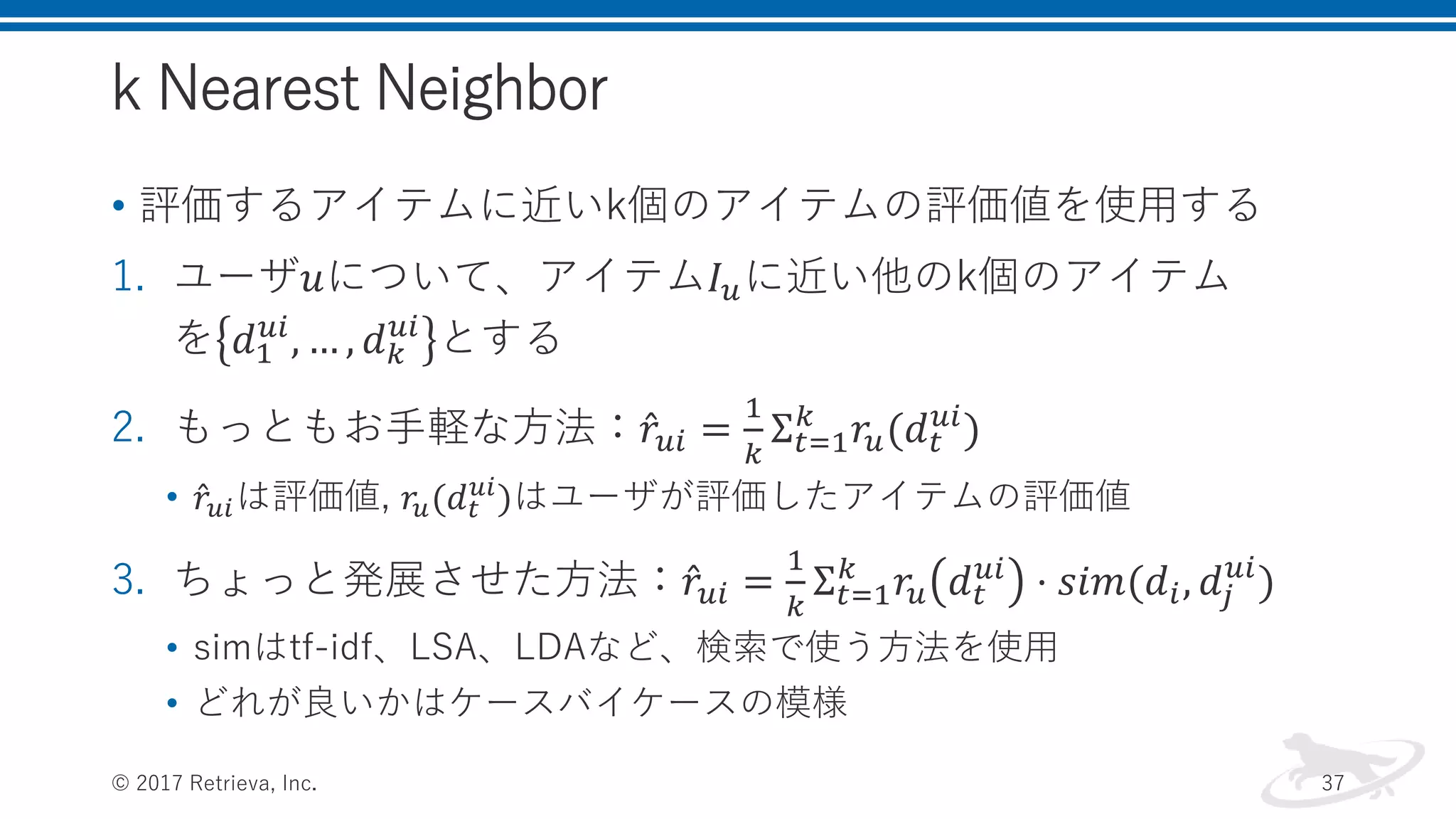
k Nearest Neighbor •
評価するアイテムに近いk個のアイテムの評価値を使用する 1. ユーザ𝑢について、アイテム𝐼 𝑢に近い他のk個のアイテム を 𝑑1 𝑢𝑖 , … , 𝑑 𝑘 𝑢𝑖 とする 2. もっともお手軽な方法: 𝑟𝑢𝑖 = 1 𝑘 Σ 𝑡=1 𝑘 𝑟𝑢(𝑑 𝑡 𝑢𝑖 ) • 𝑟𝑢𝑖は評価値, 𝑟𝑢(𝑑 𝑡 𝑢𝑖 )はユーザが評価したアイテムの評価値 3. ちょっと発展させた方法: 𝑟𝑢𝑖 = 1 𝑘 Σ 𝑡=1 𝑘 𝑟𝑢 𝑑 𝑡 𝑢𝑖 ⋅ 𝑠𝑖𝑚(𝑑𝑖, 𝑑𝑗 𝑢𝑖 ) • simはtf-idf、LSA、LDAなど、検索で使う方法を使用 • どれが良いかはケースバイケースの模様 © 2017 Retrieva, Inc. 37
38.
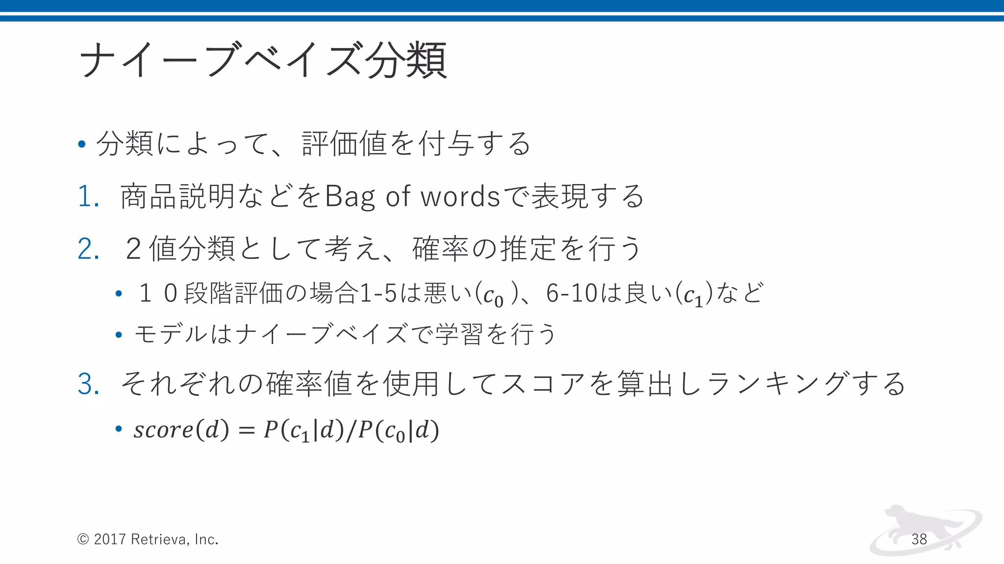
ナイーブベイズ分類 • 分類によって、評価値を付与する 1. 商品説明などをBag
of wordsで表現する 2. 2値分類として考え、確率の推定を行う • 10段階評価の場合1-5は悪い(𝑐0 )、6-10は良い(𝑐1)など • モデルはナイーブベイズで学習を行う 3. それぞれの確率値を使用してスコアを算出しランキングする • 𝑠𝑐𝑜𝑟𝑒 𝑑 = 𝑃 𝑐1 𝑑 /𝑃(𝑐0|𝑑) © 2017 Retrieva, Inc. 38
39.
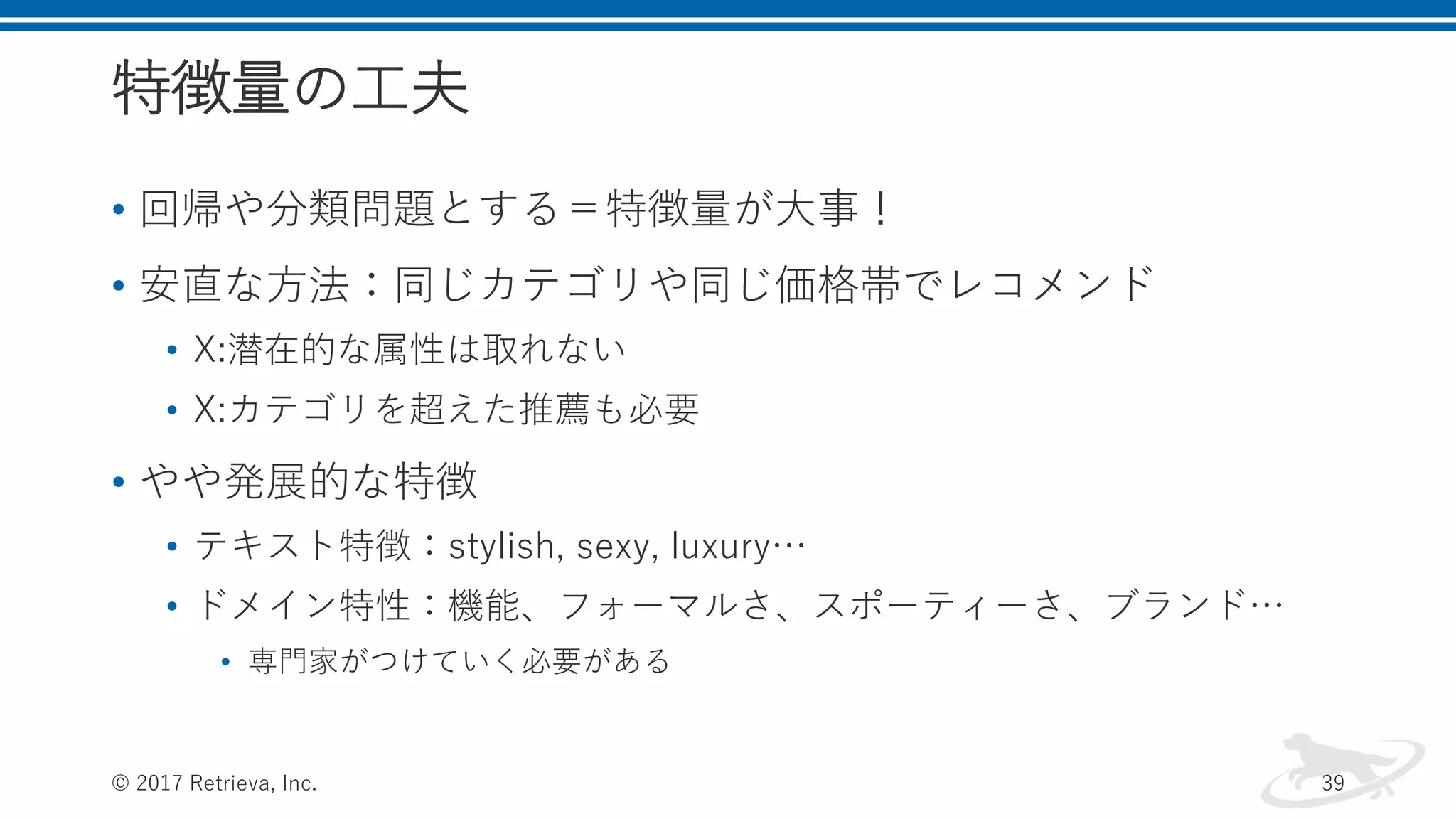
特徴量の工夫 • 回帰や分類問題とする=特徴量が大事! • 安直な方法:同じカテゴリや同じ価格帯でレコメンド •
X:潜在的な属性は取れない • X:カテゴリを超えた推薦も必要 • やや発展的な特徴 • テキスト特徴:stylish, sexy, luxury… • ドメイン特性:機能、フォーマルさ、スポーティーさ、ブランド… • 専門家がつけていく必要がある © 2017 Retrieva, Inc. 39
40.
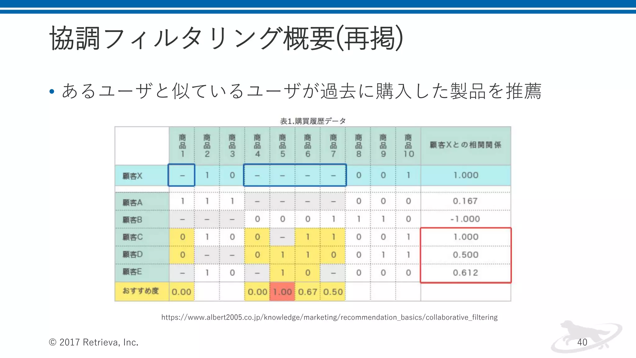
協調フィルタリング概要(再掲) • あるユーザと似ているユーザが過去に購入した製品を推薦 © 2017
Retrieva, Inc. 40 https://www.albert2005.co.jp/knowledge/marketing/recommendation_basics/collaborative_filtering
41.
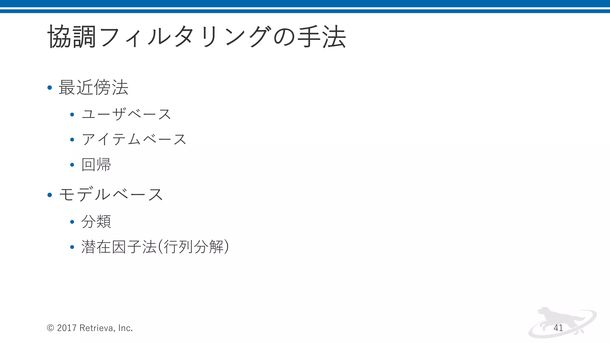
協調フィルタリングの手法 • 最近傍法 • ユーザベース •
アイテムベース • 回帰 • モデルベース • 分類 • 潜在因子法(行列分解) © 2017 Retrieva, Inc. 41
42.
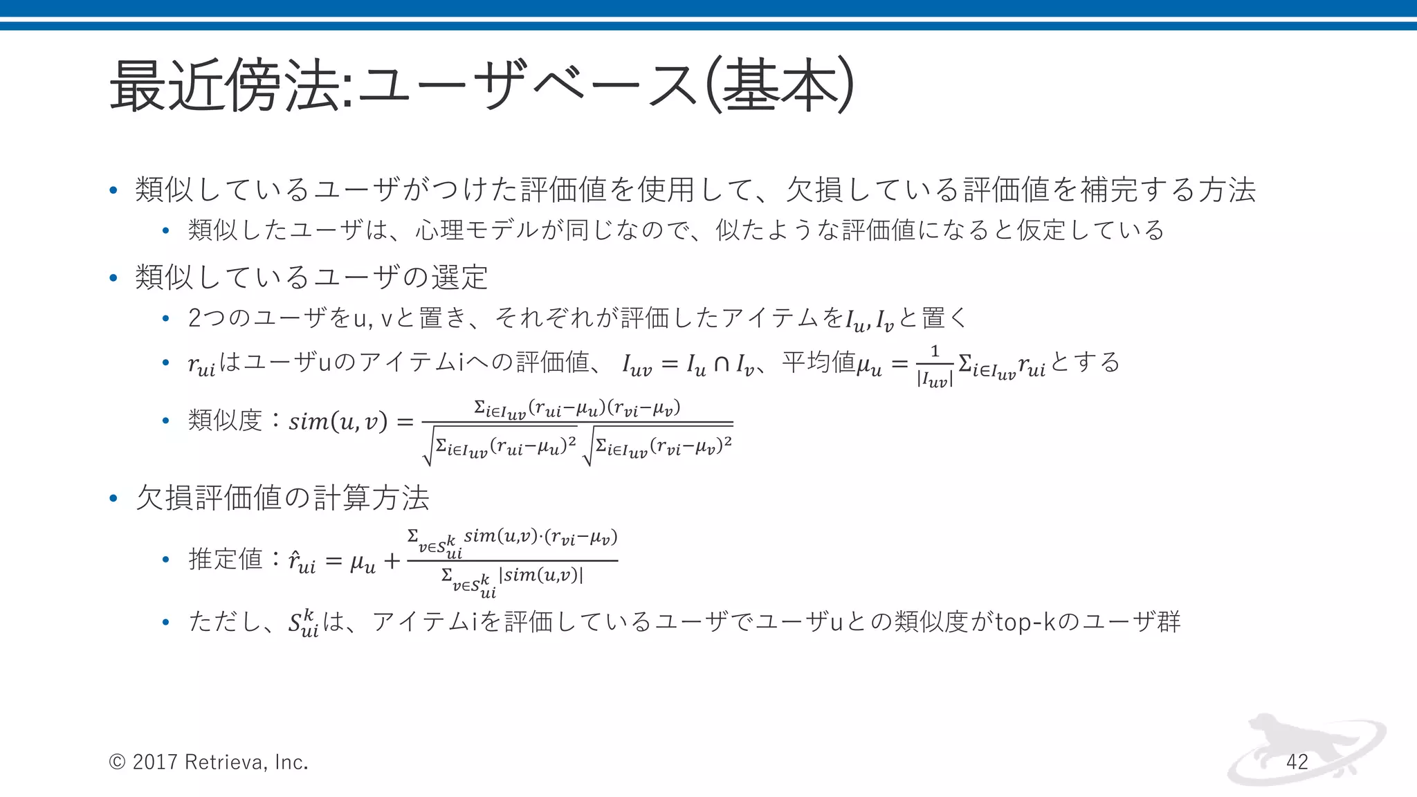
最近傍法:ユーザベース(基本) • 類似しているユーザがつけた評価値を使用して、欠損している評価値を補完する方法 • 類似したユーザは、心理モデルが同じなので、似たような評価値になると仮定している •
類似しているユーザの選定 • 2つのユーザをu, vと置き、それぞれが評価したアイテムを𝐼 𝑢, 𝐼 𝑣と置く • 𝑟𝑢𝑖はユーザuのアイテムiへの評価値、 𝐼 𝑢𝑣 = 𝐼 𝑢 ∩ 𝐼 𝑣、平均値𝜇 𝑢 = 1 𝐼 𝑢𝑣 Σ𝑖∈𝐼 𝑢𝑣 𝑟𝑢𝑖とする • 類似度:𝑠𝑖𝑚 𝑢, 𝑣 = Σ 𝑖∈𝐼 𝑢𝑣 𝑟 𝑢𝑖−𝜇 𝑢 𝑟 𝑣𝑖−𝜇 𝑣 Σ 𝑖∈𝐼 𝑢𝑣 𝑟 𝑢𝑖−𝜇 𝑢 2 Σ 𝑖∈𝐼 𝑢𝑣 𝑟 𝑣𝑖−𝜇 𝑣 2 • 欠損評価値の計算方法 • 推定値: 𝑟𝑢𝑖 = 𝜇 𝑢 + Σ 𝑣∈𝑆 𝑢𝑖 𝑘 𝑠𝑖𝑚 𝑢,𝑣 ⋅(𝑟 𝑣𝑖−𝜇 𝑣) Σ 𝑣∈𝑆 𝑢𝑖 𝑘 𝑠𝑖𝑚 𝑢,𝑣 • ただし、𝑆 𝑢𝑖 𝑘 は、アイテムiを評価しているユーザでユーザuとの類似度がtop-kのユーザ群 © 2017 Retrieva, Inc. 42
43.
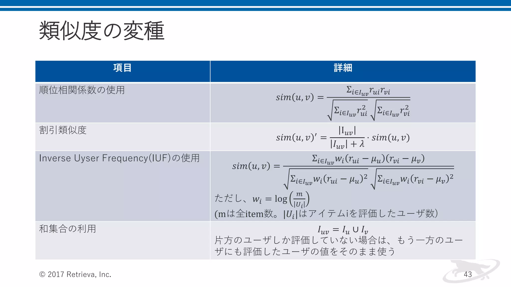
類似度の変種 項目 詳細 順位相関係数の使用 𝑠𝑖𝑚 𝑢,
𝑣 = Σ𝑖∈𝐼 𝑢𝑣 𝑟𝑢𝑖 𝑟𝑣𝑖 Σ𝑖∈𝐼 𝑢𝑣 𝑟𝑢𝑖 2 Σ𝑖∈𝐼 𝑢𝑣 𝑟𝑣𝑖 2 割引類似度 𝑠𝑖𝑚 𝑢, 𝑣 ′ = I 𝑢𝑣 𝐼 𝑢𝑣 + 𝜆 ⋅ 𝑠𝑖𝑚(𝑢, 𝑣) Inverse Uyser Frequency(IUF)の使用 𝑠𝑖𝑚 𝑢, 𝑣 = Σ𝑖∈𝐼 𝑢𝑣 𝑤𝑖 𝑟𝑢𝑖 − 𝜇 𝑢 𝑟𝑣𝑖 − 𝜇 𝑣 Σ𝑖∈𝐼 𝑢𝑣 𝑤𝑖 𝑟𝑢𝑖 − 𝜇 𝑢 2 Σ𝑖∈𝐼 𝑢𝑣 𝑤𝑖 𝑟𝑣𝑖 − 𝜇 𝑣 2 ただし、𝑤𝑖 = log 𝑚 𝑈𝑖 (mは全item数。|𝑈𝑖|はアイテムiを評価したユーザ数) 和集合の利用 𝐼 𝑢𝑣 = 𝐼 𝑢 ∪ 𝐼𝑣 片方のユーザしか評価していない場合は、もう一方のユー ザにも評価したユーザの値をそのまま使う © 2017 Retrieva, Inc. 43
44.
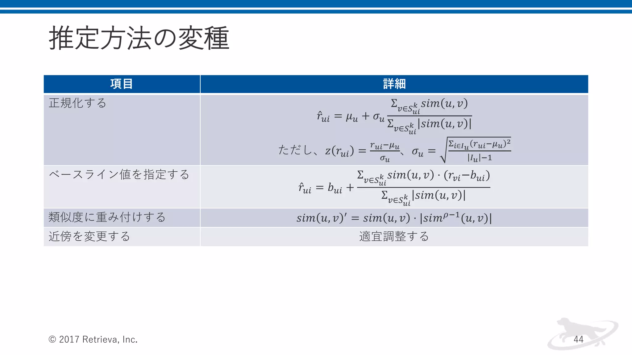
推定方法の変種 項目 詳細 正規化する 𝑟𝑢𝑖 =
𝜇 𝑢 + 𝜎 𝑢 Σ 𝑣∈𝑆 𝑢𝑖 𝑘 𝑠𝑖𝑚 𝑢, 𝑣 Σ 𝑣∈𝑆 𝑢𝑖 𝑘 𝑠𝑖𝑚 𝑢, 𝑣 ただし、𝑧 𝑟𝑢𝑖 = 𝑟 𝑢𝑖−𝜇 𝑢 𝜎 𝑢 、𝜎 𝑢 = Σ 𝑖∈𝐼 𝑢 𝑟 𝑢𝑖−𝜇 𝑢 2 𝐼 𝑢 −1 ベースライン値を指定する 𝑟𝑢𝑖 = 𝑏 𝑢𝑖 + Σ 𝑣∈𝑆 𝑢𝑖 𝑘 𝑠𝑖𝑚 𝑢, 𝑣 ⋅ (𝑟𝑣𝑖−𝑏 𝑢𝑖) Σ 𝑣∈𝑆 𝑢𝑖 𝑘 𝑠𝑖𝑚 𝑢, 𝑣 類似度に重み付けする 𝑠𝑖𝑚 𝑢, 𝑣 ′ = 𝑠𝑖𝑚 𝑢, 𝑣 ⋅ |𝑠𝑖𝑚 𝜌−1 (𝑢, 𝑣)| 近傍を変更する 適宜調整する © 2017 Retrieva, Inc. 44
45.
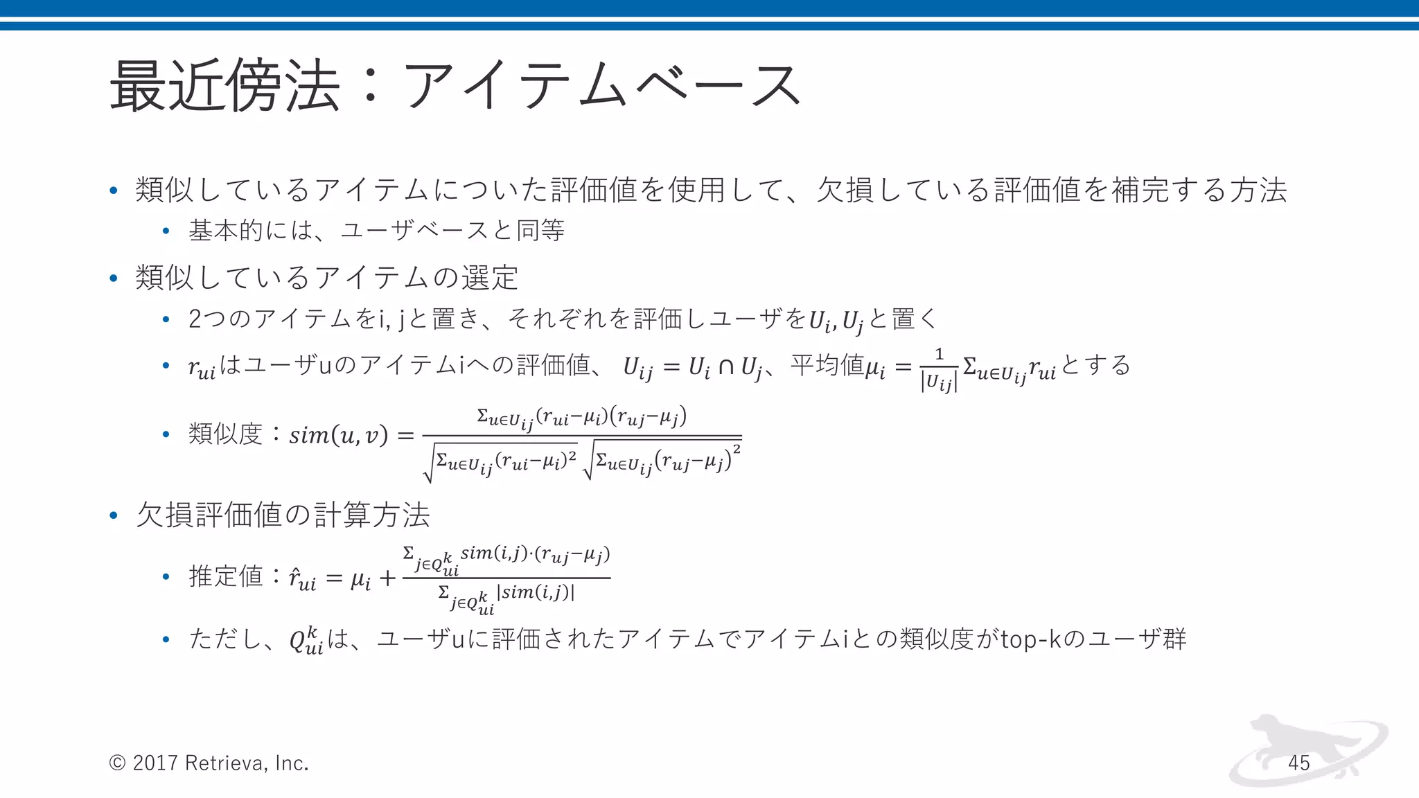
最近傍法:アイテムベース • 類似しているアイテムについた評価値を使用して、欠損している評価値を補完する方法 • 基本的には、ユーザベースと同等 •
類似しているアイテムの選定 • 2つのアイテムをi, jと置き、それぞれを評価しユーザを𝑈𝑖, 𝑈𝑗と置く • 𝑟𝑢𝑖はユーザuのアイテムiへの評価値、 𝑈𝑖𝑗 = 𝑈𝑖 ∩ 𝑈𝑗、平均値𝜇𝑖 = 1 𝑈 𝑖𝑗 Σ 𝑢∈𝑈 𝑖𝑗 𝑟𝑢𝑖とする • 類似度:𝑠𝑖𝑚 𝑢, 𝑣 = Σ 𝑢∈𝑈 𝑖𝑗 𝑟 𝑢𝑖−𝜇𝑖 𝑟 𝑢𝑗−𝜇 𝑗 Σ 𝑢∈𝑈 𝑖𝑗 𝑟 𝑢𝑖−𝜇 𝑖 2 Σ 𝑢∈𝑈 𝑖𝑗 𝑟 𝑢𝑗−𝜇 𝑗 2 • 欠損評価値の計算方法 • 推定値: 𝑟𝑢𝑖 = 𝜇𝑖 + Σ 𝑗∈𝑄 𝑢𝑖 𝑘 𝑠𝑖𝑚 𝑖,𝑗 ⋅(𝑟 𝑢𝑗−𝜇 𝑗) Σ 𝑗∈𝑄 𝑢𝑖 𝑘 𝑠𝑖𝑚 𝑖,𝑗 • ただし、𝑄 𝑢𝑖 𝑘 は、ユーザuに評価されたアイテムでアイテムiとの類似度がtop-kのユーザ群 © 2017 Retrieva, Inc. 45
46.
アイテムベースとユーザベースの比較 • ユーザベースの良さ • 何も評価していないユーザは少ない •
誰にも評価されていないアイテムはそこそこある • アイテムベースの良さ • アイテムベースの方が類似度行列が小さくなる傾向があり、 計算量的には良い © 2017 Retrieva, Inc. 46
47.
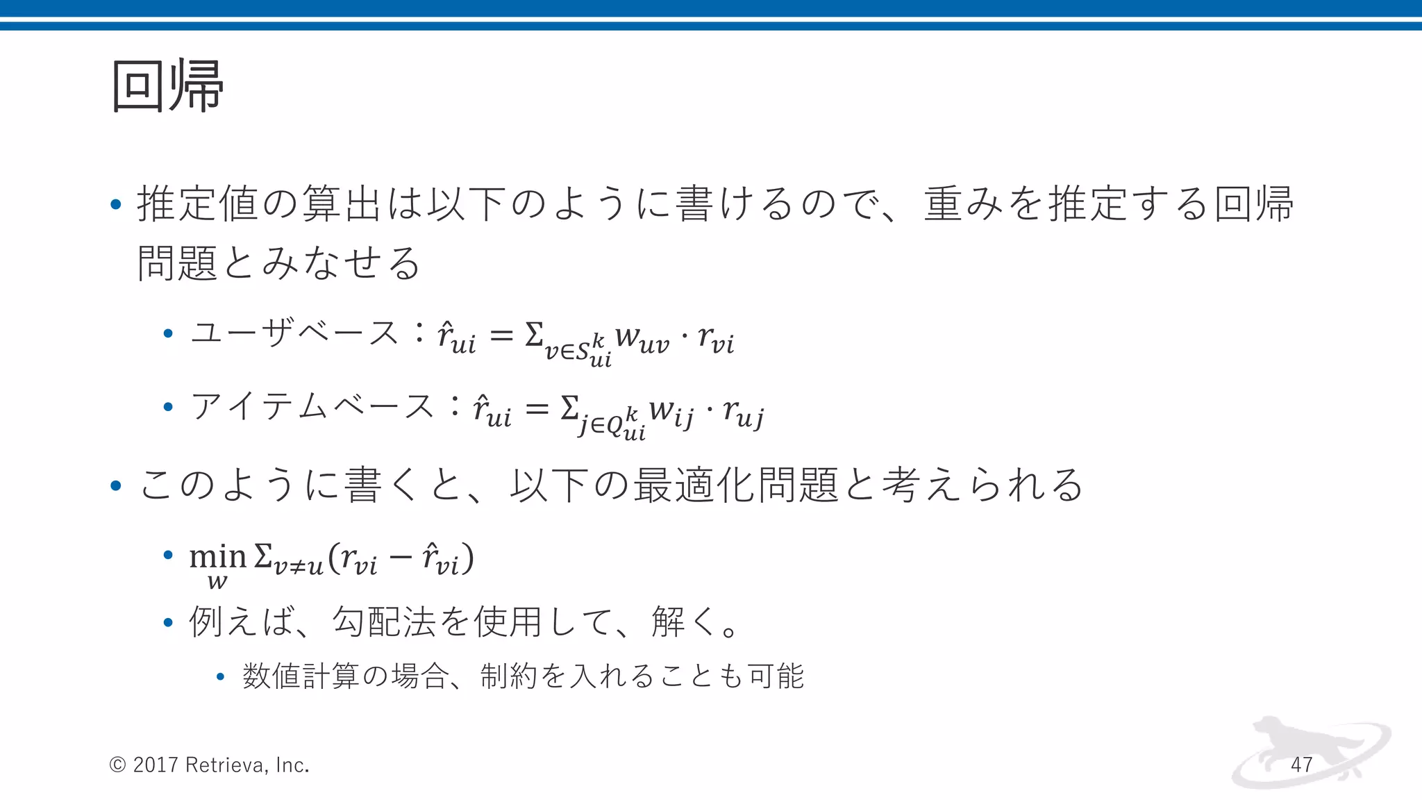
回帰 • 推定値の算出は以下のように書けるので、重みを推定する回帰 問題とみなせる • ユーザベース:
𝑟𝑢𝑖 = Σ 𝑣∈𝑆 𝑢𝑖 𝑘 𝑤 𝑢𝑣 ⋅ 𝑟𝑣𝑖 • アイテムベース: 𝑟𝑢𝑖 = Σ𝑗∈𝑄 𝑢𝑖 𝑘 𝑤𝑖𝑗 ⋅ 𝑟𝑢𝑗 • このように書くと、以下の最適化問題と考えられる • min 𝑤 Σ 𝑣≠𝑢(𝑟𝑣𝑖 − 𝑟𝑣𝑖) • 例えば、勾配法を使用して、解く。 • 数値計算の場合、制約を入れることも可能 © 2017 Retrieva, Inc. 47
48.
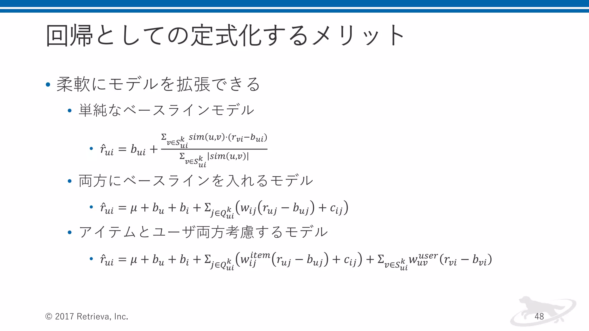
回帰としての定式化するメリット • 柔軟にモデルを拡張できる • 単純なベースラインモデル •
𝑟𝑢𝑖 = 𝑏 𝑢𝑖 + Σ 𝑣∈𝑆 𝑢𝑖 𝑘 𝑠𝑖𝑚 𝑢,𝑣 ⋅(𝑟 𝑣𝑖−𝑏 𝑢𝑖) Σ 𝑣∈𝑆 𝑢𝑖 𝑘 𝑠𝑖𝑚 𝑢,𝑣 • 両方にベースラインを入れるモデル • 𝑟𝑢𝑖 = 𝜇 + 𝑏 𝑢 + 𝑏𝑖 + Σ𝑗∈𝑄 𝑢𝑖 𝑘 𝑤𝑖𝑗 𝑟𝑢𝑗 − 𝑏 𝑢𝑗 + 𝑐𝑖𝑗 • アイテムとユーザ両方考慮するモデル • 𝑟𝑢𝑖 = 𝜇 + 𝑏 𝑢 + 𝑏𝑖 + Σ𝑗∈𝑄 𝑢𝑖 𝑘 𝑤𝑖𝑗 𝑖𝑡𝑒𝑚 𝑟𝑢𝑗 − 𝑏 𝑢𝑗 + 𝑐𝑖𝑗 + Σ 𝑣∈𝑆 𝑢𝑖 𝑘 𝑤 𝑢𝑣 𝑢𝑠𝑒𝑟 𝑟𝑣𝑖 − 𝑏 𝑣𝑖 © 2017 Retrieva, Inc. 48
49.
モデルベース • 最近傍法の限界 • スパースデータに対して性能が出ない(距離が似たり寄ったり) •
オンラインとオフラインの計算部分を切り分けづらい • モデルベース(機械学習の活用)へ • 最近傍より精度が良いことが多い • 次元削減をすることで、安定性を向上させる • モデルの学習と評価でオンライン・オフラインを分けられる • ナイーブベイズ等を使う © 2017 Retrieva, Inc. 49
50.
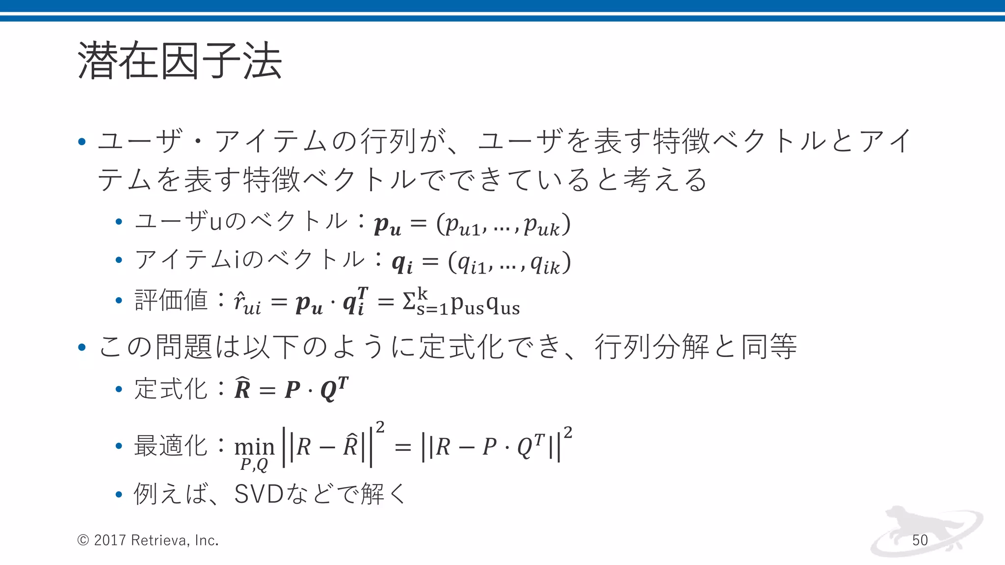
潜在因子法 • ユーザ・アイテムの行列が、ユーザを表す特徴ベクトルとアイ テムを表す特徴ベクトルでできていると考える • ユーザuのベクトル:𝒑
𝒖 = (𝑝 𝑢1, … , 𝑝 𝑢𝑘) • アイテムiのベクトル:𝒒𝒊 = (𝑞𝑖1, … , 𝑞𝑖𝑘) • 評価値: 𝑟𝑢𝑖 = 𝒑 𝒖 ⋅ 𝒒𝒊 𝑻 = Σs=1 k pusqus • この問題は以下のように定式化でき、行列分解と同等 • 定式化: 𝑹 = 𝑷 ⋅ 𝑸 𝑻 • 最適化:min 𝑃,𝑄 𝑅 − 𝑅 2 = 𝑅 − 𝑃 ⋅ 𝑄 𝑇 2 • 例えば、SVDなどで解く © 2017 Retrieva, Inc. 50
51.
レコメンドエンジンのチューニング © 2017 Retrieva,
Inc. 51
52.
概要 • その他:多目的化 © 2017
Retrieva, Inc. 52 パーソナライズする パーソナライズしない コンテキストを使う • コンテキストを使わない手法に以下3つを組み合わせる 1. Pre-Filtering 2. Post-Filetering 3. モデリング コンテキストを使わない • 協調フィルタリング • 内容ベースレコメンド • 両者の組み合わせ • 類似度計算 • トレンド計算 • 頻度計算 • アソシエーション
53.
両者の組みわせ • 良いレコメンドのためには、より豊富な情報を考慮する必要が ある • 協調フィルタリングはコンテンツ情報を無視しており、内容ベースレ コメンドは、評価行列の方法を無視している •
注意点:必ずしも組み合わせる必要はない(UIでカバーすれば良い) • 代表的な方法 • スイッチング • ブレンディング © 2017 Retrieva, Inc. 53
54.
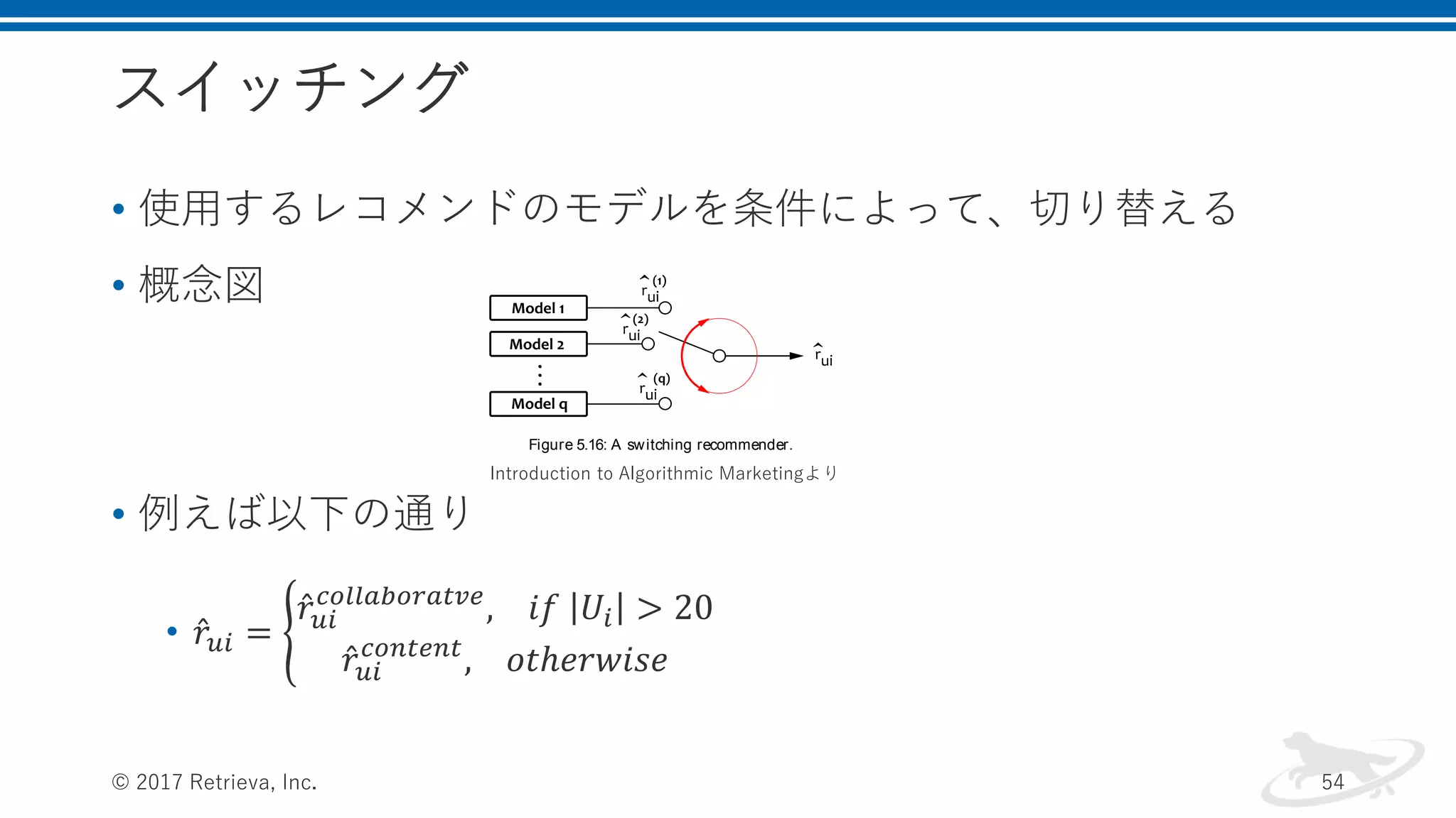
スイッチング • 使用するレコメンドのモデルを条件によって、切り替える • 概念図 •
例えば以下の通り • 𝑟𝑢𝑖 = 𝑟𝑢𝑖 𝑐𝑜𝑙𝑙𝑎𝑏𝑜𝑟𝑎𝑡𝑣𝑒 , 𝑖𝑓 𝑈𝑖 > 20 𝑟𝑢𝑖 𝑐𝑜𝑛𝑡𝑒𝑛𝑡 , 𝑜𝑡ℎ𝑒𝑟𝑤𝑖𝑠𝑒 © 2017 Retrieva, Inc. 54 r (content) u i , otherwise in which Ui is the set of users who rated item i. This solution can help us to work around the cold-start problem, which is an issue for collaborative filtering, and, at the same time, to improve trivial rec- ommendations produced by content-based filtering whenever possible. A generic schema of such a switching recommender is shown in Fig- ure 5.16. This approach, however, is somewhat rudimentary because it is based on heuristic rules rather than a formal optimization frame- work. We can definitely achieve better results by leveraging machine learning and optimization algorithms to properly mix the outputs of the individual models. Figure 5.16: A switching recommender. 5.9.2 Blending Let us assume that several recommendation models have been trained for the same set of users and items, so each of these models can es- timate rating ru i for a given pair of user and item. Our goal is to combine these estimates together to produce the final rating estimate, which is, ideally, more accurate than the predictions produced by any single one of the models. This can be done by using heuristic rules, as we did in the switching approach described in the previous section, but, at the same time, it is naturally a regression problem that can be efficiently solved by using the machine learning toolkit. The problem of blending several rating estimates together can be for- mally defined in the following way. Let us assume that we have s train- ing samples, that is, known rating values in the training set. This set is Introduction to Algorithmic Marketingより
55.
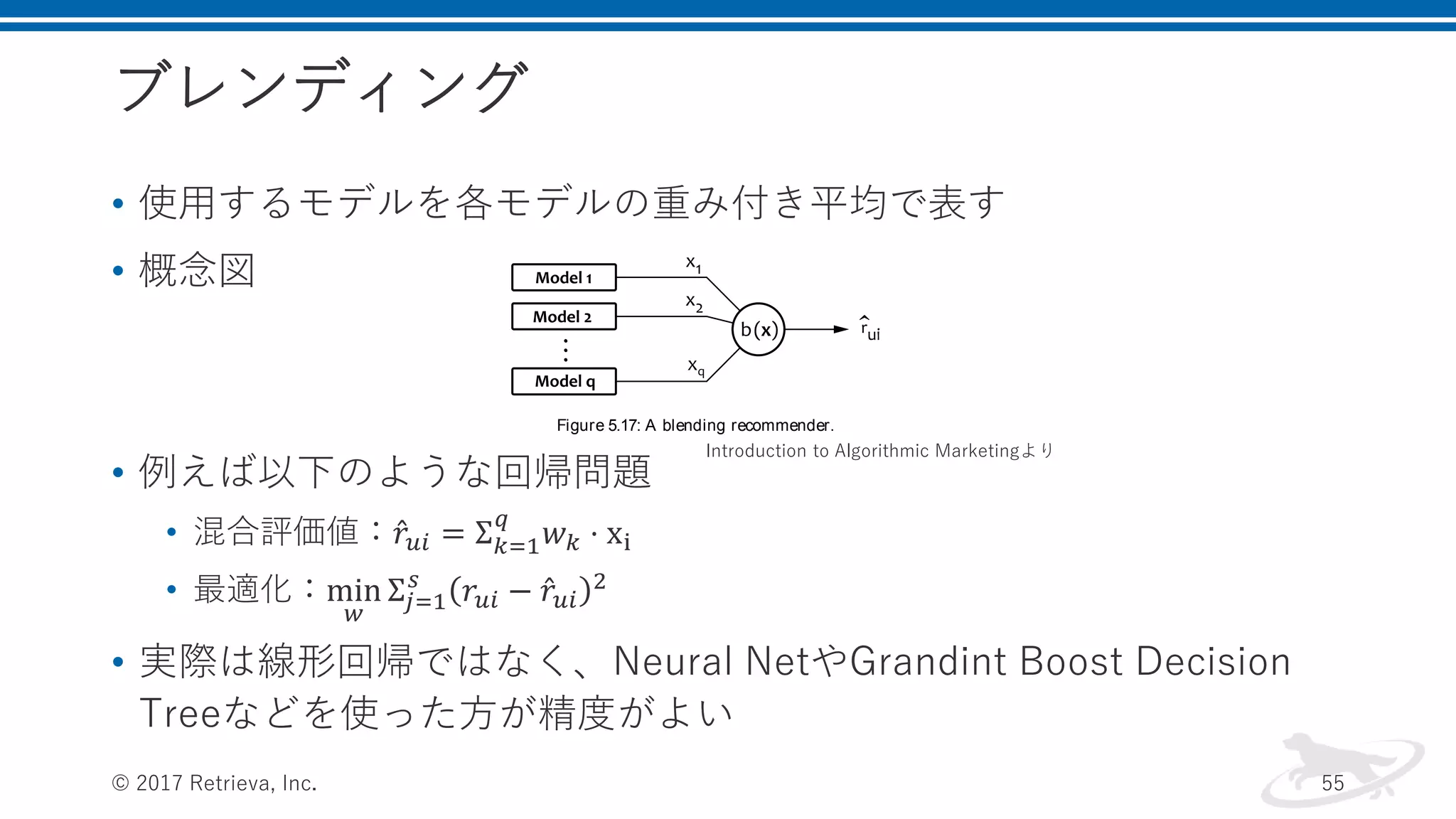
ブレンディング • 使用するモデルを各モデルの重み付き平均で表す • 概念図 •
例えば以下のような回帰問題 • 混合評価値: 𝑟𝑢𝑖 = Σ 𝑘=1 𝑞 𝑤 𝑘 ⋅ xi • 最適化:min 𝑤 Σ𝑗=1 𝑠 𝑟𝑢𝑖 − 𝑟𝑢𝑖 2 • 実際は線形回帰ではなく、Neural NetやGrandint Boost Decision Treeなどを使った方が精度がよい © 2017 Retrieva, Inc. 55 b x that minimizes the prediction error: min b s j 1 b xj yj 2 (5.122) This view of the problem is illustrated in Figure 5.17. This prob- lem, that is, the combination of the predictions of several learning al- gorithms by using another learning algorithm, is known as stacking, so we use the terms blending and stacking interchangeably. Stacking is es- sentially a standard supervised learning problem that can be solved by using a variety of classification or regression algorithms. Figure 5.17: A blending recommender. One of the most basic solutions of problem 5.122 is, of course, lin- ear regression. In this case, the combiner function is a linear function defined as b x xT w (5.123) in which w is the vector of model weights. In other words, the final rating prediction is a linear combination of predictions produced by individual recommendation algorithms: ru i q k 1 wk r k u i (5.124) The optimal weights for the blending function can be straightfor- wardly calculated by using ridge regression: T 1 T Introduction to Algorithmic Marketingより
56.
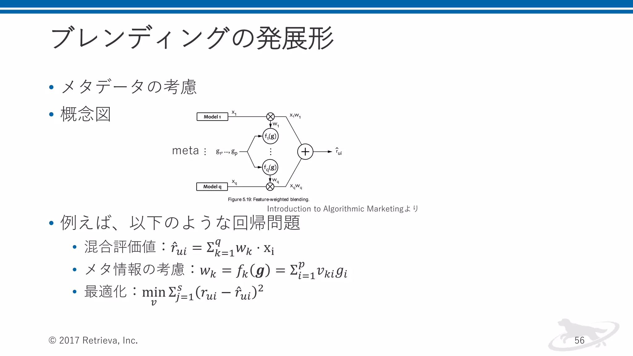
ブレンディングの発展形 • メタデータの考慮 • 概念図 •
例えば、以下のような回帰問題 • 混合評価値: 𝑟𝑢𝑖 = Σ 𝑘=1 𝑞 𝑤 𝑘 ⋅ xi • メタ情報の考慮:𝑤 𝑘 = 𝑓𝑘 𝒈 = Σ𝑖=1 𝑝 𝑣 𝑘𝑖 𝑔𝑖 • 最適化:min 𝑣 Σ𝑗=1 𝑠 𝑟𝑢𝑖 − 𝑟𝑢𝑖 2 © 2017 Retrieva, Inc. 56 associated with each rating value. We choose to mix the predictions by using the linear blending function b x q k 1 wk xk (5.126) but weights wk are dynamically calculated based on the meta- features: wk fk g p i 1 vk i gi (5.127) in which fk are called feature functions and vk i are static weights. In other words, the feature functions amplify or suppress the signals from the recommendation models, as shown in Figure 5.19. Note that this design is quite similar to the signal mixing pipelines that we discussed in Chapter 4, in the context of search services. Figure 5.19: Feature-weighted blending. meta Introduction to Algorithmic Marketingより
57.
コンテキスト情報を使ったレコメンド 種類 概念図 普通のレコメンド Pre-filtering Post-filtering モデリング © 2017
Retrieva, Inc. 57 ing channels that the system is integrated with. Some other attributes, especially intent-related ones, may not be directly available but can be obtained by using special features of the user interface (for example, a This is a gift order checkbox on an online order placement form) or inferred by using predictive models. 5.10.2 Context-AwareRecommendation Techniques A non-contextual recommendation service can be viewed as a process that consumes the training data in the form User Item Rating, cre- ates a model that maps the pair of user and item to rating, and evalu- ates this model for a given user to produce a sorted list of recommen- dations. This pipeline is shown in Figure 5.21. Figure 5.21: The main steps of the non-contextual recommendation process [Adomavicius and Tuzhilin, 2008]. U , I , and R are the dimensions of users, items, and ratings, respectively. Recommended items are denoted as i , j ,. . . The multidimensional framework described in the previous section suggests several ideas for how this pipeline can be modified to incor- porate contextual information [Adomavicius and Tuzhilin, 2008]: con t ext ual pr ef i l t er i n g The first possible solution is to create a two-dimensional rating matrix from the original multidimen- sional data and then apply a standard non-contextual recom- mendation model or algorithm with this matrix as an input, as shown in Figure 5.22. The rating matrix is a slice of the multidi- mensional cube selected for a given value of the context. For ex- ample, a movie recommendation service that stores ratings with time stamps can make recommendations on the weekdays and weekends by using two different matrices. The matrices are cre- ated by selecting all weekday or all weekend ratings, respectively, from the original data cube.
58.
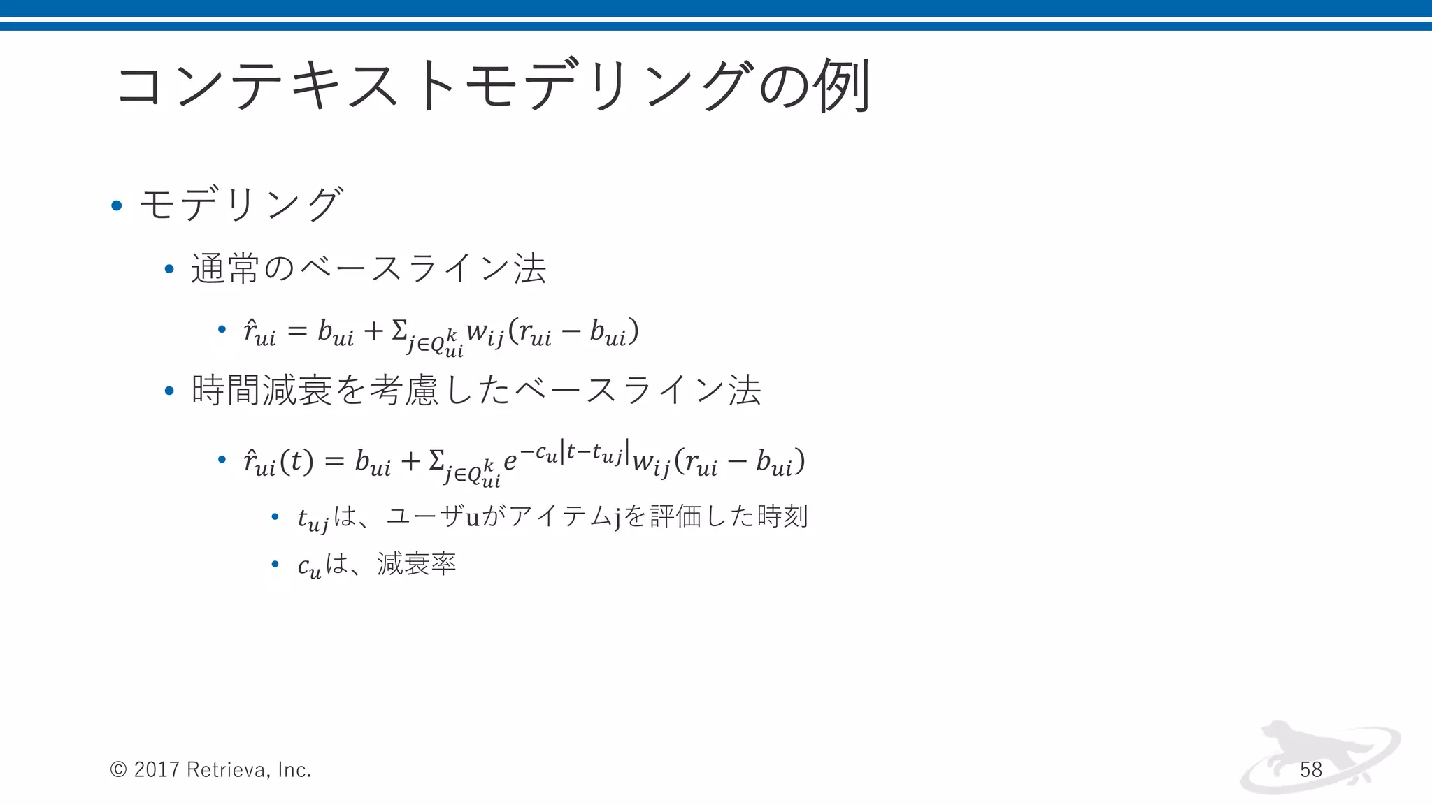
コンテキストモデリングの例 • モデリング • 通常のベースライン法 •
𝑟𝑢𝑖 = 𝑏 𝑢𝑖 + Σ𝑗∈𝑄 𝑢𝑖 𝑘 𝑤𝑖𝑗 𝑟𝑢𝑖 − 𝑏 𝑢𝑖 • 時間減衰を考慮したベースライン法 • 𝑟𝑢𝑖(𝑡) = 𝑏 𝑢𝑖 + Σ𝑗∈𝑄 𝑢𝑖 𝑘 𝑒−𝑐 𝑢 𝑡−𝑡 𝑢𝑗 𝑤𝑖𝑗 𝑟𝑢𝑖 − 𝑏 𝑢𝑖 • 𝑡 𝑢𝑗は、ユーザuがアイテムjを評価した時刻 • 𝑐 𝑢は、減衰率 © 2017 Retrieva, Inc. 58
59.
まとめ © 2017 Retrieva,
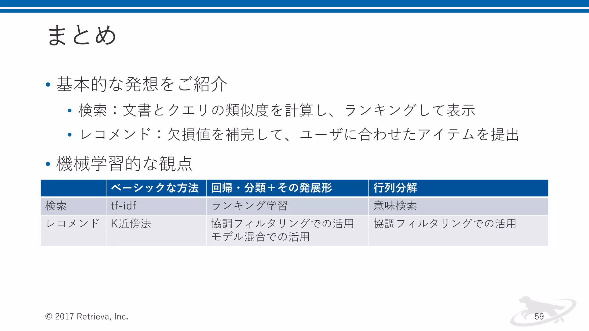
Inc. 59 • 基本的な発想をご紹介 • 検索:文書とクエリの類似度を計算し、ランキングして表示 • レコメンド:欠損値を補完して、ユーザに合わせたアイテムを提出 • 機械学習的な観点 ベーシックな方法 回帰・分類+その発展形 行列分解 検索 tf-idf ランキング学習 意味検索 レコメンド K近傍法 協調フィルタリングでの活用 モデル混合での活用 協調フィルタリングでの活用
60.
Appendix:検索の評価指標 © 2017 Retrieva,
Inc. 60
61.
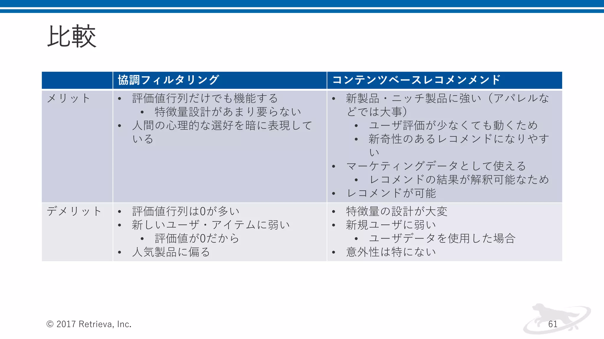
比較 協調フィルタリング コンテンツベースレコメンメンド メリット •
評価値行列だけでも機能する • 特徴量設計があまり要らない • 人間の心理的な選好を暗に表現して いる • 新製品・ニッチ製品に強い(アパレルな どでは大事) • ユーザ評価が少なくても動くため • 新奇性のあるレコメンドになりやす い • マーケティングデータとして使える • レコメンドの結果が解釈可能なため • レコメンドが可能 デメリット • 評価値行列は0が多い • 新しいユーザ・アイテムに弱い • 評価値が0だから • 人気製品に偏る • 特徴量の設計が大変 • 新規ユーザに弱い • ユーザデータを使用した場合 • 意外性は特にない © 2017 Retrieva, Inc. 61
62.
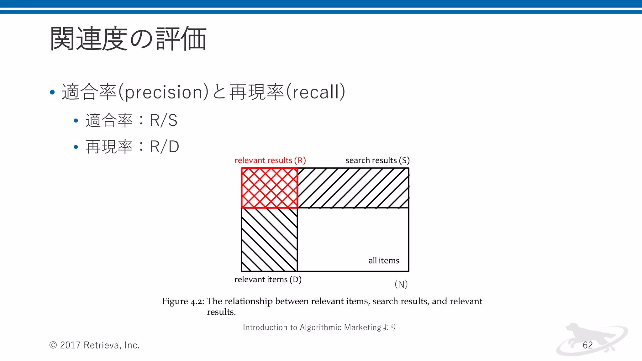
関連度の評価 • 適合率(precision)と再現率(recall) • 適合率:R/S •
再現率:R/D © 2017 Retrieva, Inc. 62 (N) Introduction to Algorithmic Marketingより
63.
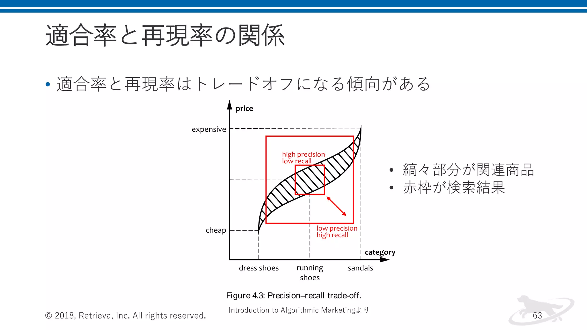
適合率と再現率の関係 • 適合率と再現率はトレードオフになる傾向がある © 2018,
Retrieva, Inc. All rights reserved. 63 4.2 busi n ess obj ect i ves 187 Figure 4.3: Precision–recall trade-off. calculate the precision and recall at each point, and plot a precision– Introduction to Algorithmic Marketingより • 縞々部分が関連商品 • 赤枠が検索結果
64.
(参考)検索の単一指標 • Mean Average
Precision(MAP) • Cumurative Gain(CG) • Discouted Cumurative Gain(DCG) • Normalized Discouted Cumurative Gain(DCG) © 2017 Retrieva, Inc. 64
65.
ビジネス目的によるリランキング • Boost and
Bury • Filtering • Canned Results • Redirection • Product Grouping © 2017 Retrieva, Inc. 65
66.
UXおよびCS • Conversion Rate •
Click-Though Rate • Time on A Product Detail Page • Query Modification Rate • Paging Rate • Retention Rate • Search Latency © 2017 Retrieva, Inc. 66
67.
© 2017 Retrieva,
Inc.
Download


![発展的な方法
• Embedding:単語を表現するベクトルを、連続値で表現する
• 今まで:𝒗 𝒕 = [0,0, . . , 0,1,0, … , 0]
• Embedding: 𝒗 𝒕 = [0.3,0.2, … , −0.04]
• 連続値のベクトルで表現することの効果
• クエリに出現していないへの近さも考慮できる
• その結果、精度が悪くなる場合も
• クエリに入っていても、意味的に遠い単語は除外できる
• Embeddingの精度とその後の計算方法が合っていれば
• そのままクエリに使える
• Embeddingの作成方法→LSA、pLSA、LDA、Word2Vec
© 2017 Retrieva, Inc. 9](https://image.slidesharecdn.com/introductiontosearchandrecommendalgolithm-181128012613/75/Introduction-to-search_and_recommend_algolithm-9-2048.jpg)


![コンテキスト情報を使ったレコメンド
種類 概念図
普通のレコメンド
Pre-filtering
Post-filtering
モデリング
© 2017 Retrieva, Inc. 57
ing channels that the system is integrated with. Some other attributes,
especially intent-related ones, may not be directly available but can be
obtained by using special features of the user interface (for example,
a This is a gift order checkbox on an online order placement form) or
inferred by using predictive models.
5.10.2 Context-AwareRecommendation Techniques
A non-contextual recommendation service can be viewed as a process
that consumes the training data in the form User Item Rating, cre-
ates a model that maps the pair of user and item to rating, and evalu-
ates this model for a given user to produce a sorted list of recommen-
dations. This pipeline is shown in Figure 5.21.
Figure 5.21: The main steps of the non-contextual recommendation process
[Adomavicius and Tuzhilin, 2008]. U , I , and R are the dimensions
of users, items, and ratings, respectively. Recommended items are
denoted as i , j ,. . .
The multidimensional framework described in the previous section
suggests several ideas for how this pipeline can be modified to incor-
porate contextual information [Adomavicius and Tuzhilin, 2008]:
con t ext ual pr ef i l t er i n g The first possible solution is to create
a two-dimensional rating matrix from the original multidimen-
sional data and then apply a standard non-contextual recom-
mendation model or algorithm with this matrix as an input, as
shown in Figure 5.22. The rating matrix is a slice of the multidi-
mensional cube selected for a given value of the context. For ex-
ample, a movie recommendation service that stores ratings with
time stamps can make recommendations on the weekdays and
weekends by using two different matrices. The matrices are cre-
ated by selecting all weekday or all weekend ratings, respectively,
from the original data cube.](https://image.slidesharecdn.com/introductiontosearchandrecommendalgolithm-181128012613/75/Introduction-to-search_and_recommend_algolithm-57-2048.jpg)


![[DSO]勉強会_データサイエンス講義_Chapter8](https://cdn.slidesharecdn.com/ss_thumbnails/data-science-lecture-chapter8-ver2-191018120312-thumbnail.jpg?width=640&height=640&fit=bounds)