27. Physics Grade 9 StudentTextbook Final version.pdf
Introduction to mechanics_and_
1. This is page i
Printer: Opaque this
Introduction to
Mechanics and Symmetry
A Basic Exposition of Classical Mechanical Systems
Second Edition
Jerrold E. Marsden
and
Tudor S. Ratiu
Last modified on 15 July 1998
2. v
To Barbara and Lilian for their love and support
........................... 15 July 1998—18h02 ...........................
4. This is page ix
Printer: Opaque this
Preface
Symmetry and mechanics have been close partners since the time of the
founding masters: Newton, Euler, Lagrange, Laplace, Poisson, Jacobi, Ha-
milton, Kelvin, Routh, Riemann, Noether, Poincar´, Einstein, Schr¨dinger,
e o
Cartan, Dirac, and to this day, symmetry has continued to play a strong
role, especially with the modern work of Kolmogorov, Arnold, Moser, Kir-
illov, Kostant, Smale, Souriau, Guillemin, Sternberg, and many others. This
book is about these developments, with an emphasis on concrete applica-
tions that we hope will make it accessible to a wide variety of readers,
especially senior undergraduate and graduate students in science and en-
gineering.
The geometric point of view in mechanics combined with solid analy-
sis has been a phenomenal success in linking various diverse areas, both
within and across standard disciplinary lines. It has provided both insight
into fundamental issues in mechanics (such as variational and Hamiltonian
structures in continuum mechanics, fluid mechanics, and plasma physics)
and provided useful tools in specific models such as new stability and bifur-
cation criteria using the energy-Casimir and energy-momentum methods,
new numerical codes based on geometrically exact update procedures and
variational integrators, and new reorientation techniques in control theory
and robotics.
Symmetry was already widely used in mechanics by the founders of the
subject, and has been developed considerably in recent times in such di-
verse phenomena as reduction, stability, bifurcation and solution symmetry
breaking relative to a given system symmetry group, methods of finding
explicit solutions for integrable systems, and a deeper understanding of spe-
5. x Preface
cial systems, such as the Kowalewski top. We hope this book will provide
a reasonable avenue to, and foundation for, these exciting developments.
Because of the extensive and complex set of possible directions in which
one can develop the theory, we have provided a fairly lengthy introduction.
It is intended to be read lightly at the beginning and then consulted from
time to time as the text itself is read.
This volume contains much of the basic theory of mechanics and should
prove to be a useful foundation for further, as well as more specialized
topics. Due to space limitations we warn the reader that many important
topics in mechanics are not treated in this volume. We are preparing a
second volume on general reduction theory and its applications. With luck,
a little support, and yet more hard work, it will be available in the near
future.
Solutions Manual. A solution manual is available for insturctors that
contains complete solutions to many of the exercises and other supplemen-
tary comments. This may be obtained from the publisher.
Internet Supplements. To keep the size of the book within reason,
we are making some material available (free) on the internet. These are
a collection of sections whose omission does not interfere with the main
flow of the text. See http://www.cds.caltech.edu/~marsden. Updates
and information about the book can also be found there.
What is New in the Second Edition? In this second edition, the
main structural changes are the creation of the Solutions manual (along
with many more Exercises in the text) and the internet supplements. The
internet supplements contain, for example, the material on the Maslov in-
dex that was not needed for the main flow of the book. As for the substance
of the text, much of the book was rewritten throughout to improve the flow
of material and to correct inaccuracies. Some examples: the material on the
Hamilton-Jacobi theory was completely rewritten, a new section on Routh
reduction (§8.9) was added, Chapter 9 on Lie groups was substantially im-
proved and expanded and the presentation of examples of coadjoint orbits
(Chapter 14) was improved by stressing matrix methods throughout.
Acknowledgments. We thank Alan Weinstein, Rudolf Schmid, and Rich
Spencer for helping with an early set of notes that helped us on our way.
Our many colleagues, students, and readers, especially Henry Abarbanel,
Vladimir Arnold, Larry Bates, Michael Berry, Tony Bloch, Hans Duister-
maat, Marty Golubitsky, Mark Gotay, George Haller, Aaron Hershman,
Darryl Holm, Phil Holmes, Sameer Jalnapurkar, Edgar Knobloch, P.S.
Krishnaprasad, Naomi Leonard, Debra Lewis, Robert Littlejohn, Richard
Montgomery, Phil Morrison, Richard Murray, Peter Olver, Oliver O’Reilly,
Juan-Pablo Ortega, George Patrick, Octavian Popp, Matthias Reinsch,
Shankar Sastry, Juan Simo, Hans Troger, and Steve Wiggins have our deep-
est gratitude for their encouragement and suggestions. We also collectively
........................... 15 July 1998—18h02 ...........................
6. xi
thank all our students and colleagues who have used these notes and have
provided valuable advice. We are also indebted to Carol Cook, Anne Kao,
Nawoyuki Gregory Kubota, Sue Knapp, Barbara Marsden, Marnie McEl-
hiney, June Meyermann, Teresa Wild, and Ester Zack for their dedicated
and patient work on the typesetting and artwork for this book. We want
to single out with special thanks, Nawoyuki Gregory Kubota and Wendy
McKay for their special effort with the typesetting and the figures (includ-
ing the cover illustration). We also thank the staff at Springer-Verlag, espe-
cially Achi Dosanjh, Laura Carlson, Ken Dreyhaupt and R¨diger Gebauer
u
for their skillful editorial work and production of the book.
Jerry Marsden
Pasadena, California
Tudor Ratiu
Santa Cruz, California
Summer, 1998
........................... 15 July 1998—18h02 ...........................
7. xii
About the Authors
Jerrold E. Marsden is Professor of Control and Dynamical Systems at Caltech.
He got his B.Sc. at Toronto in 1965 and his Ph.D. from Princeton University in
1968, both in Applied Mathematics. He has done extensive research in mechan-
ics, with applications to rigid body systems, fluid mechanics, elasticity theory,
plasma physics as well as to general field theory. His primary current interests
are in the area of dynamical systems and control theory, especially how it relates
to mechanical systems with symmetry. He is one of the founders in the early
1970’s of reduction theory for mechanical systems with symmetry, which remains
an active and much studied area of research today. He was the recipient of the
prestigious Norbert Wiener prize of the American Mathematical Society and the
Society for Industrial and Applied Mathematics in 1990, and was elected a fellow
of the AAAS in 1997. He has been a Carnegie Fellow at Heriot–Watt Univer-
sity (1977), a Killam Fellow at the University of Calgary (1979), recipient of the
Jeffrey–Williams prize of the Canadian Mathematical Society in 1981, a Miller
Professor at the University of California, Berkeley (1981–1982), a recipient of the
Humboldt Prize in Germany (1991), and a Fairchild Fellow at Caltech (1992). He
has served in several administrative capacities, such as director of the Research
Group in Nonlinear Systems and Dynamics at Berkeley, 1984–86, the Advisory
Panel for Mathematics at NSF, the Advisory committee of the Mathematical Sci-
ences Institute at Cornell, and as Director of The Fields Institute, 1990–1994. He
has served as an Editor for Springer-Verlag’s Applied Mathematical Sciences Se-
ries since 1982 and serves on the editorial boards of several journals in mechanics,
dynamics, and control.
Tudor S. Ratiu is Professor of Mathematics at UC Santa Cruz and the Swiss
Federal Institute of Technology in Lausanne. He got his B.Sc. in Mathematics and
M.Sc. in Applied Mathematics, both at the University of Timi¸oara, Romania,
s
and his Ph.D. in Mathematics at Berkeley in 1980. He has previously taught at
the University of Michigan, Ann Arbor, as a T. H. Hildebrandt Research Assis-
tant Professor (1980–1983) and at the University of Arizona, Tucson (1983–1987).
His research interests center on geometric mechanics, symplectic geometry, global
analysis, and infinite dimensional Lie theory, together with their applications to
integrable systems, nonlinear dynamics, continuum mechanics, plasma physics,
and bifurcation theory. He has been a National Science Foundation Postdoctoral
Fellow (1983–86), a Sloan Foundation Fellow (1984–87), a Miller Research Pro-
fessor at Berkeley (1994), and a recipient of of the Humboldt Prize in Germany
(1997). Since his arrival at UC Santa Cruz in 1987, he has been on the executive
committee of the Nonlinear Sciences Organized Research Unit. He is currently
managing editor of the AMS Surveys and Monographs series and on the edito-
rial board of the Annals of Global Analysis and the Annals of the University of
Timi¸oara. He was also a member of various research institutes such as MSRI in
s
Berkeley, the Center for Nonlinear Studies at Los Alamos, the Max Planck Insti-
tute in Bonn, MSI at Cornell, IHES in Bures–sur–Yvette, The Fields Institute in
Toronto (Waterloo), the Erwin Schro¨dinger Institute for Mathematical Physics
o
in Vienna, the Isaac Newton Institute in Cambridge, and RIMS in Kyoto.
........................... 15 July 1998—18h02 ...........................
15. This is page 1
Printer: Opaque this
1
Introduction and Overview
1.1 Lagrangian and Hamiltonian Formalisms
Mechanics deals with the dynamics of particles, rigid bodies, continuous
media (fluid, plasma, and solid mechanics), and field theories such as elec-
tromagnetism, gravity, etc. This theory plays a crucial role in quantum
mechanics, control theory, and other areas of physics, engineering and even
chemistry and biology. Clearly mechanics is a large subject that plays a
fundamental role in science. Mechanics also played a key part in the devel-
opment of mathematics. Starting with the creation of calculus stimulated
by Newton’s mechanics, it continues today with exciting developments in
group representations, geometry, and topology; these mathematical devel-
opments in turn are being applied to interesting problems in physics and
engineering.
Symmetry plays an important role in mechanics, from fundamental for-
mulations of basic principles to concrete applications, such as stability cri-
teria for rotating structures. The theme of this book is to emphasize the
role of symmetry in various aspects of mechanics.
This introduction treats a collection of topics fairly rapidly. The student
should not expect to understand everything perfectly at this stage. We will
return to many of the topics in subsequent chapters.
Lagrangian and Hamiltonian Mechanics. Mechanics has two main
points of view, Lagrangian mechanics and Hamiltonian mechanics.
In one sense, Lagrangian mechanics is more fundamental since it is based
on variational principles and it is what generalizes most directly to the
16. 2 1. Introduction and Overview
general relativistic context. In another sense, Hamiltonian mechanics is
more fundamental, since it is based directly on the energy concept and it is
what is more closely tied to quantum mechanics. Fortunately, in many cases
these branches are equivalent as we shall see in detail in Chapter 7. Needless
to say, the merger of quantum mechanics and general relativity remains
one of the main outstanding problems of mechanics. In fact, the methods
of mechanics and symmetry are important ingredients in the developments
of string theory that has attempted this merger.
Lagrangian Mechanics. The Lagrangian formulation of mechanics is
based on the observation that there are variational principles behind the
fundamental laws of force balance as given by Newton’s law F = ma.
One chooses a configuration space Q with coordinates q i , i = 1, . . . , n,
that describe the configuration of the system under study. Then one
introduces the Lagrangian L(q i , q i , t), which is shorthand notation for
˙
L(q 1 , . . . , q n , q 1 , . . . , q n , t). Usually, L is the kinetic minus the potential
˙ ˙
energy of the system and one takes q i = dq i /dt to be the system velocity.
˙
The variational principle of Hamilton states
b
δ L(q i , q i , t) dt = 0.
˙ (1.1.1)
a
In this principle, we choose curves q i (t) joining two fixed points in Q over
a fixed time interval [a, b], and calculate the integral regarded as a function
of this curve. Hamilton’s principle states that this function has a critical
point at a solution within the space of curves. If we let δq i be a variation,
that is, the derivative of a family of curves with respect to a parameter,
then by the chain rule, (1.1.1) is equivalent to
n b
∂L i ∂L i
δq + i δ q dt = 0
˙ (1.1.2)
i=1 a ∂q i ∂q
˙
for all variations δq i .
Using equality of mixed partials, one finds that
d i
δq . δqi =
˙
dt
Using this, integrating the second term of (1.1.2) by parts, and employing
the boundary conditions δq i = 0 at t = a and b, (1.1.2) becomes
n b
∂L d ∂L
− δq i dt = 0. (1.1.3)
i=1 a ∂q i dt ∂ qi
˙
Since δq i is arbitrary (apart from being zero at the endpoints), (1.1.2) is
equivalent to the Euler–Lagrange equations
d ∂L ∂L
− i = 0, i = 1, . . . , n. (1.1.4)
dt ∂ q i
˙ ∂q
........................... 15 July 1998—18h02 ...........................
17. 1.1 Lagrangian and Hamiltonian Formalisms 3
As Hamilton himself realized around 1830, one can also gain valuable in-
formation by not imposing the fixed endpoint conditions. We will have a
deeper look at such issues in Chapters 7 and 8.
For a system of N particles moving in Euclidean 3-space, we choose the
configuration space to be Q = R3N = R3 × · · · × R3 (N times) and L often
has the form of kinetic minus potential energy:
N
1
˙
L(qi , qi , t) = ˙
mi qi 2
− V (qi ), (1.1.5)
2 i=1
where we write points in Q as q1 , . . . , qN , where qi ∈ R3 . In this case the
Euler–Lagrange equations (1.1.4) reduce to Newton’s second law
d ∂V
(mi qi ) = −
˙ ; i = 1, . . . , N (1.1.6)
dt ∂qi
that is, F = ma for the motion of particles in the potential field V . As we
shall see later, in many examples more general Lagrangians are needed.
Generally, in Lagrangian mechanics, one identifies a configuration space
Q (with coordinates q 1 , . . . , q n )) and then forms the velocity phase space
T Q also called the tangent bundle of Q. Coordinates on T Q are denoted
(q 1 , . . . , q n , q 1 , . . . , q n ),
˙ ˙
and the Lagrangian is regarded as a function L : T Q → R.
Already at this stage, interesting links with geometry are possible. If
gij (q) is a given metric tensor or mass matrix (for now, just think of this
as a q-dependent positive-definite symmetric n×n matrix) and we consider
the kinetic energy Lagrangian
n
1
L(q i , q i ) =
˙ gij (q)q i q j ,
˙ ˙ (1.1.7)
2 i,j=1
then the Euler–Lagrange equations are equivalent to the equations of geodesic
motion, as can be directly verified (see §7.5 for details). Conservation laws
that are a result of symmetry in a mechanical context can then be applied
to yield interesting geometric facts. For instance, theorems about geodesics
on surfaces of revolution can be readily proved this way.
The Lagrangian formalism can be extended to the infinite dimensional
case. One view (but not the only one) is to replace the q i by fields ϕ1 , . . . , ϕm
which are, for example, functions of spatial points xi and time. Then L
is a function of ϕ1 , . . . , ϕm , ϕ1 , . . . , ϕm and the spatial derivatives of the
˙ ˙
fields. We shall deal with various examples of this later, but we emphasize
that properly interpreted, the variational principle and the Euler–Lagrange
equations remain intact. One replaces the partial derivatives in the Euler–
Lagrange equations by functional derivatives defined below.
........................... 15 July 1998—18h02 ...........................
18. 4 1. Introduction and Overview
Hamiltonian Mechanics. To pass to the Hamiltonian formalism, in-
troduce the conjugate momenta
∂L
pi = , i = 1, . . . , n, (1.1.8)
∂ qi
˙
make the change of variables (q i , q i ) → (q i , pi ), and introduce the Hamil-
˙
tonian
n
H(q i , pi , t) = pj q j − L(q i , q i , t).
˙ ˙ (1.1.9)
j=1
Remembering the change of variables, we make the following computations
using the chain rule:
n
∂H ∂ qj
˙ ∂L ∂ q j
˙
= qi +
˙ pj − j = qi
˙ (1.1.10)
∂pi j=1
∂pi ∂ q ∂pi
˙
and
n n
∂H ∂ qj
˙ ∂L ∂L ∂ q j
˙ ∂L
= pj − i− = − i, (1.1.11)
∂q i j=1
∂q i ∂q j=1
∂ q j ∂q i
˙ ∂q
where (1.1.8) has been used twice. Using (1.1.4) and (1.1.8), we see that
(1.1.11) is equivalent to
∂H d
= − pi . (1.1.12)
∂q i dt
Thus, the Euler–Lagrange equations are equivalent to Hamilton’s equa-
tions
dq i ∂H
= ,
dt ∂pi
(1.1.13)
dpi ∂H
=− i,
dt ∂q
where i = 1, . . . , n. The analogous Hamiltonian partial differential equa-
tions for time dependent fields ϕ1 , . . . , ϕm and their conjugate momenta
π1 , ..., πm , are
∂ϕa δH
=
∂t δπa
(1.1.14)
∂πa δH
= − a,
∂t δϕ
........................... 15 July 1998—18h02 ...........................
19. 1.1 Lagrangian and Hamiltonian Formalisms 5
where a = 1, . . . , m, and H is a functional of the fields ϕa and πa , and the
variational or functional derivatives are defined by the equation
δH 1 n 1
δϕ d x = lim [H(ϕ1 +εδϕ1 , ϕ2 , . . . , ϕm , π1 , . . . , πm )
Rn δϕ1 ε→0 ε
− H(ϕ1 , ϕ2 , . . . , ϕm , π1 , . . . , πm )], (1.1.15)
and similarly for δH/δϕ2 , . . . , δH/δπm . Equations (1.1.13) and (1.1.14) can
be recast in Poisson bracket form
˙
F = {F, H}, (1.1.16)
where the brackets in the respective cases are given by
n
∂F ∂G ∂F ∂G
{F, G} = − (1.1.17)
i=1
∂q i ∂pi ∂pi ∂q i
and
m
δF δG δF δG
{F, G} = − dn x. (1.1.18)
a=1 Rn δϕa δπa δπa δϕa
Associated to any configuration space Q (coordinatized by (q 1 , . . . , q n ))
is a phase space T ∗ Q called the cotangent bundle of Q, which has coordi-
nates (q 1 , . . . , q n , p1 , . . . , pn ). On this space, the canonical bracket (1.1.17)
is intrinsically defined in the sense that the value of {F, G} is indepen-
dent of the choice of coordinates. Because the Poisson bracket satisfies
{F, G} = −{G, F } and in particular {H, H} = 0 , we see from (1.1.16)
˙
that H = 0; that is, energy is conserved . This is the most elementary
of many deep and beautiful conservation properties of mechanical sys-
tems.
There is also a variational principle on the Hamiltonian side. For the
Euler–Lagrange equations, we deal with curves in q-space (configuration
space), whereas for Hamilton’s equations we deal with curves in (q, p)-space
(momentum phase space). The principle is
b n
δ [pi q i − H(q j , pj )] dt = 0
˙ (1.1.19)
a i=1
as is readily verified; one requires pi δq i = 0 at the endpoints.
This formalism is the basis for the analysis of many important systems
in particle dynamics and field theory, as described in standard texts such
as Whittaker [1927], Goldstein [1980], Arnold [1989], Thirring [1978], and
Abraham and Marsden [1978]. The underlying geometric structures that are
important for this formalism are those of symplectic and Poisson geometry.
........................... 15 July 1998—18h02 ...........................
20. 6 1. Introduction and Overview
How these structures are related to the Euler–Lagrange equations and vari-
ational principles via the Legendre transformation is an essential ingredient
of the story. Furthermore, in the infinite-dimensional case it is fairly well
understood how to deal rigorously with many of the functional analytic
difficulties that arise; see, for example, Chernoff and Marsden [1974] and
Marsden and Hughes [1983].
Exercises
1.1-1. Show by direct calculation that the classical Poisson bracket sat-
isfies the Jacobi identity . That is, if F and K are both functions of the
2n variables (q 1 , q 2 , . . . , q n , p1 , p2 , ..., pn ) and we define
n
∂F ∂K ∂K ∂F
{F, K} = − i ,
i=1
∂q i ∂pi ∂q ∂pi
then the identity {L, {F, K}} + {K, {L, F }} + {F, {K, L}} = 0 holds.
1.2 The Rigid Body
It was already clear in the last century that certain mechanical systems
resist the canonical formalism outlined in §1.1. For example, to obtain a
Hamiltonian description for fluids, Clebsch [1857, 1859] found it necessary
to introduce certain nonphysical potentials1 . We will discuss fluids in §1.4
below.
Euler’s Rigid Body Equations. In the absence of external forces, the
Euler equations for the rotational dynamics of a rigid body about its cen-
ter of mass are usually written as follows, as we shall derive in detail in
Chapter 15:
˙
I1 Ω1 = (I2 − I3 )Ω2 Ω3 ,
˙
I2 Ω2 = (I3 − I1 )Ω3 Ω1 , (1.2.1)
˙
I3 Ω3 = (I1 − I2 )Ω1 Ω2 ,
where Ω = (Ω1 , Ω2 , Ω3 ) is the body angular velocity vector (the angular
velocity of the rigid body as seen from a frame fixed in the body) and
I1 , I2 , I3 are constants depending on the shape and mass distribution of
the body—the principal moments of inertia of the rigid body.
1 For a geometric account of Clebsch potentials and further references, see Marsden
and Weinstein [1983], Marsden, Ratiu, and Weinstein [1984a,b], Cendra and Marsden
[1987], and Cendra, Ibort, and Marsden [1987].
........................... 15 July 1998—18h02 ...........................
21. 1.2 The Rigid Body 7
Are equations (1.2.1) Lagrangian or Hamiltonian in any sense? Since
there are an odd number of equations, they obviously cannot be put in
canonical Hamiltonian form in the sense of equations (1.1.13).
A classical way to see the Lagrangian (or Hamiltonian) structure of the
rigid body equations is to use a description of the orientation of the body
˙ ˙ ˙
in terms of three Euler angles denoted θ, ϕ, ψ and their velocities θ, ϕ, ψ
(or conjugate momenta pθ , pϕ , pψ ), relative to which the equations are in
Euler–Lagrange (or canonical Hamiltonian) form. However, this procedure
requires using six equations while many questions are easier to study using
the three equations (1.2.1).
Lagrangian Form. To see the sense in which (1.2.1) are Lagrangian,
introduce the Lagrangian
1
L(Ω) = (I1 Ω2 + I2 Ω2 + I3 Ω2 )
1 2 3 (1.2.2)
2
which, as we will see in detail in Chapter 15, is the (rotational) kinetic
energy of the rigid body. Regarding IΩ = (I1 Ω1 , I2 Ω2 , I3 Ω3 ) as a vector,
write (1.2.1) as
d ∂L ∂L
= × Ω. (1.2.3)
dt ∂Ω ∂Ω
These equations appear explicitly in Lagrange [1788] (Volume 2, p.212)
and were generalized to arbitrary Lie algebras by Poincar´ [1901b]. We will
e
discuss these general Euler-Poincar´ equations in Chapter 13. We can
e
also write a variational principle for (1.2.3) that is analogous to that for the
Euler–Lagrange equations, but is written directly in terms of Ω. Namely,
(1.2.3) is equivalent to
b
δ L dt = 0, (1.2.4)
a
where variations of Ω are restricted to be of the form
˙
δΩ = Σ + Ω × Σ, (1.2.5)
where Σ is a curve in R3 that vanishes at the endpoints. This may be
proved in the same way as we proved that the variational principle (1.1.1)
is equivalent to the Euler–Lagrange equations (1.1.4); see Exercise 1.2-2.
In fact, later on in Chapter 13, we shall see how to derive this variational
principle from the more “primitive” one (1.1.1).
Hamiltonian Form. If, instead of variational principles, we concentrate
on Poisson brackets and drop the requirement that they be in the canon-
ical form (1.1.17), then there is also a simple and beautiful Hamiltonian
........................... 15 July 1998—18h02 ...........................
22. 8 1. Introduction and Overview
structure for the rigid body equations. To state it, introduce the angular
momenta
∂L
Πi = Ii Ωi = , i = 1, 2, 3, (1.2.6)
∂Ωi
so that the Euler equations become
˙ I2 − I3
Π1 = Π2 Π3 ,
I2 I3
˙ I3 − I1
Π2 = Π3 Π1 , (1.2.7)
I3 I1
˙ I1 − I2
Π3 = Π1 Π2 ,
I1 I2
that is,
˙
Π = Π × Ω. (1.2.8)
Introduce the following rigid body Poisson bracket on functions of the
Π’s:
{F, G}(Π) = −Π · ( F × G) (1.2.9)
and the Hamiltonian
1 Π2
1 Π2 Π2
H= + 2+ 3 . (1.2.10)
2 I1 I2 I3
One checks (Exercise 1.2-3) that Euler’s equations (1.2.7) are equivalent
to2
˙
F = {F, H}. (1.2.11)
For any equation of the form (1.2.11), conservation of total angular mo-
mentum holds regardless of the Hamiltonian; indeed, with
1 2
C(Π) = (Π + Π2 + Π2 ),
2 1 2 3
we have C(Π) = Π, and so
d 1 2
(Π + Π2 + Π2 ) = {C, H}(Π)
dt 2 1 2 3
= −Π · ( C × H)
= −Π · (Π × H) = 0.
2 This simple result is implicit in many works, such as Arnold [1966, 1969], and is
given explicitly in this form for the rigid body in Sudarshan and Mukunda [1974]. (Some
preliminary versions were given by Pauli [1953], Martin [1959], and Nambu [1973].) On
the other hand, the variational form (1.2.4) appears to be due to Poincar´ [1901b] and
e
Hamel [1904], at least implicitly. It is given explicitly for fluids in Newcomb [1962] and
Bretherton [1970] and in the general case in Marsden and Scheurle [1993a,b].
........................... 15 July 1998—18h02 ...........................
23. 1.2 The Rigid Body 9
The same calculation shows that {C, F } = 0 for any F . Functions such
as these that Poisson commute with every function are called Casimir
functions; they play an important role in the study of stability, as we
shall see later3 .
Exercises
1.2-1. Show by direct calculation that the rigid body Poisson bracket
satisfies the Jacobi identity. That is, if F and K are both functions of
(Π1 , Π2 , Π3 ) and we define
{F, K}(Π) = −Π · ( F × K),
then the identity {L, {F, K}} + {K, {L, F }} + {F, {K, L}} = 0 holds.
1.2-2. Verify directly that the Euler equations for a rigid body are equiv-
alent to
δ L dt = 0
˙
for variations of the form δΩ = Σ + Ω × Σ, where Σ vanishes at the
endpoints.
1.2-3. Verify directly that the Euler equations for a rigid body are equiv-
alent to the equations
d
F = {F, H},
dt
where { , } is the rigid body Poisson bracket and H is the rigid body Hamil-
tonian.
1.2-4.
(a) Show that the rotation group SO(3) can be identified with the Poin-
car´ sphere: that is, the unit circle bundle of the two sphere S 2 ,
e
defined to be the set of unit tangent vectors to the two-sphere in R3 .
(b) Using the known fact from basic topolgy that any (continuous) vec-
tor field on S 2 must vanish somewhere, show that SO(3) cannot be
written as S 2 × S 1 .
3 H. B. G. Casimir was a student of P. Ehrenfest and wrote a brilliant thesis on
the quantum mechanics of the rigid body, a problem that has not been adequately
addressed in the detail that would be desirable, even today. Ehrenfest in turn wrote his
thesis under Boltzmann around 1900 on variational principles in fluid dynamics and was
one of the first to study fluids from this point of view in material, rather than Clebsch
representation. Curiously, Ehrenfest used the Gauss–Hertz principle of least curvature
rather than the more elementary Hamilton prinicple. This is a seed for many important
ideas in this book.
........................... 15 July 1998—18h02 ...........................
24. 10 1. Introduction and Overview
1.3 Lie–Poisson Brackets,
Poisson Manifolds, Momentum Maps
The rigid body variational principle and the rigid body Poisson bracket
are special cases of general constructions associated to any Lie algebra g,
that is, a vector space together with a bilinear, antisymmetric bracket [ξ, η]
satisfying Jacobi’s identity :
[[ξ, η], ζ] + [[ζ, ξ], η] + [[η, ζ], ξ] = 0 (1.3.1)
for all ξ, η, ζ ∈ g. For example, the Lie algebra associated to the rotation
group is g = R3 with bracket [ξ, η] = ξ × η, the ordinary vector cross
product.
The Euler-Poincar´ Equations.
e The construction of a variational prin-
ciple on g, replaces
˙
δΩ = Σ + Ω × Σ by δξ = η + [η, ξ].
˙
The resulting general equations on g, which we will study in detail in Chap-
ter 13, are called the Euler-Poincar´ equations. These equations are
e
valid for either finite or infinite dimensional Lie algebras. To state them in
the finite dimensional case, we use the following notation. Choosing a basis
d
e1 , . . . , er of g (so dim g = r), the structure constants Cab are defined
by the equation
r
d
[ea , eb ] = Cab ed , (1.3.2)
d=1
where a, b run from 1 to r. If ξ is an element of the Lie algebra, its compo-
nents relative to this basis are denoted ξ a . If e1 , . . . , er is the corresponding
dual basis, then the components of the differential of the Lagrangian L are
the partial derivatives ∂L/∂ξ a . Then the Euler-Poincar´ equations are
e
r
d ∂L b ∂L a
= Cad ξ . (1.3.3)
dt ∂ξ d ∂ξ b
a,b=1
The coordinate-free version reads
d ∂L ∂L
= ad∗
ξ ,
dt ∂ξ ∂ξ
where adξ : g → g is the linear map η → [ξ, η] and ad∗ : g∗ → g∗ is its
ξ
dual. For example, for L : R3 → R, the Euler-Poincar´ equations become
e
d ∂L ∂L
= × Ω,
dt ∂Ω ∂Ω
........................... 15 July 1998—18h02 ...........................
25. 1.3 Lie–Poisson Brackets, Poisson Manifolds, Momentum Maps 11
which generalize the Euler equations for rigid body motion. As we men-
tioned earlier, these equations were written down for a fairly general class
of L by Lagrange [1788, Volume 2, Equation A on p. 212], while it was
Poincar´ [1901b] who generalized them to any Lie algebra.
e
The generalization of the rigid body variational principle states that the
Euler–Poincar´ equations are equivalent to
e
δ L dt = 0 (1.3.4)
for all variations of the form δξ = η + [ξ, η] for some curve η in g that
˙
vanishes at the end points.
The Lie–Poisson Equations. We can also generalize the rigid body
Poisson bracket as follows: Let F, G be defined on the dual space g∗ . De-
noting elements of g∗ by µ, let the functional derivative of F at µ be
the unique element δF/δµ of g defined by
1 δF
lim [F (µ + εδµ) − F (µ)] = δµ, , (1.3.5)
ε→0ε δµ
for all δµ ∈ g∗ , where , denotes the pairing between g∗ and g. This
definition (1.3.5) is consistent with the definition of δF/δϕ given in (1.1.15)
when g and g∗ are chosen to be appropriate spaces of fields. Define the (±)
Lie–Poisson brackets by
δF δG
{F, G}± (µ) = ± µ, , . (1.3.6)
δµ δµ
Using the coordinate notation introduced above, the (±) Lie–Poisson brack-
ets become
r
∂F ∂G
{F, G}± (µ) = ± d
Cab µd , (1.3.7)
∂µa ∂µb
a,b,d=1
where µ = µa ea .
Poisson Manifolds. The Lie–Poisson bracket and the canonical brackets
from the last section have four simple but crucial properties:
PB1 {F, G} is real bilinear in F and G.
PB2 {F, G} = −{G, F }, antisymmetry.
PB3 {F, G}, H} + {{H, F }, G} + {{G, H}, F } = 0, Jacobi identity.
PB4 {F G, H} = F {G, H} + {F, H}G, Leibniz identity.
A manifold (that is, an n-dimensional “smooth surface”) P together
with a bracket operation on F(P ), the space of smooth functions on P ,
........................... 15 July 1998—18h02 ...........................
26. 12 1. Introduction and Overview
and satisfying properties PB1–PB4, is called a Poisson manifold . In
particular, g∗ is a Poisson manifold . In Chapter 10 we will study the general
concept of a Poisson manifold.
For example, if we choose g = R3 with the bracket taken to be the cross
product [x, y] = x × y, and identify g∗ with g using the dot product on R3
(so Π, x = Π · x is the usual dot product), then the (−) Lie–Poisson
bracket becomes the rigid body bracket.
Hamiltonian Vector Fields. On a Poisson manifold (P, {· , ·}), associ-
ated to any function H there is a vector field, denoted by XH , which has
the property that for any smooth function F : P → R we have the identity
dF, XH = dF · XH = {F, H}.
where dF is the differential fo F . We say that the vector field XH is gener-
ated by the function H or that XH is the Hamiltonian vector field as-
sociated with H. We also define the associated dynamical system whose
points z in phase space evolve in time by the differential equation
z = XH (z).
˙ (1.3.8)
This definition is consistent with the equations in Poisson bracket form
(1.1.16). The function H may have the interpretation of the energy of the
system, but of course the definition (1.3.8) makes sense for any function.
For canonical systems with the Poisson bracket given by (1.1.17), XH is
given by the formula
∂H ∂H
XH (q i , pi ) = ,− i , (1.3.9)
∂pi ∂q
whereas for the rigid body bracket given on R3 by (1.2.9),
XH (Π) = Π × H(Π). (1.3.10)
˙
The general Lie–Poisson equations, determined by F = {F, H} read
r
d ∂H
µa =
˙ µd Cab ,
∂µb
b,c=1
or intrinsically,
µ=
˙ ad∗
δH/δµ µ. (1.3.11)
Reduction. There is an important feature of the rigid body bracket that
also carries over to more general Lie algebras, namely, Lie–Poisson brackets
arise from canonical brackets on the cotangent bundle (phase space) T ∗ G
associated with a Lie group G which has g as its associated Lie algebra.
........................... 15 July 1998—18h02 ...........................
27. 1.3 Lie–Poisson Brackets, Poisson Manifolds, Momentum Maps 13
(The general theory of Lie groups is presented in Chapter 9.) Specifically,
there is a general construction underlying the association
(θ, ϕ, ψ, pθ , pϕ , pψ ) → (Π1 , Π2 , Π3 ) (1.3.12)
defined by:
1
Π1 = [(pϕ − pψ cos θ) sin ψ + pθ sin θ cos ψ],
sin θ
1 (1.3.13)
Π2 = [(pϕ − pψ cos θ) cos ψ − pθ sin θ sin ψ],
sin θ
Π 3 = pψ .
This rigid body map takes the canonical bracket in the variables (θ, ϕ, ψ)
and their conjugate momenta (pθ , pϕ , pψ ) to the (−) Lie–Poisson bracket in
the following sense. If F and K are functions of Π1 , Π2 , Π3 , they determine
functions of (θ, ϕ, ψ, pθ , pϕ , pψ ) by substituting (1.3.13). Then a (tedious
but straightforward) exercise using the chain rule shows that
{F, K}(−){Lie-Poisson} = {F, K}canonical . (1.3.14)
We say that the map defined by (1.3.13) is a canonical map or a
Poisson map and that the (−) Lie–Poisson bracket has been obtained
from the canonical bracket by reduction.
For a rigid body free to rotate about is center of mass, G is the (proper)
rotation group SO(3) and the Euler angles and their conjugate momenta
are coordinates for T ∗ G. The choice of T ∗ G as the primitive phase space is
made according to the classical procedures of mechanics: the configuration
space SO(3) is chosen since each element A ∈ SO(3) describes the orien-
tation of the rigid body relative to a reference configuration, that is, the
rotation A maps the reference configuration to the current configuration.
For the description using Lagrangian mechanics, one forms the velocity-
˙ ˙ ˙
phase space T SO(3) with coordinates (θ, ϕ, ψ, θ, ϕ, ψ). The Hamiltonian
description is obtained as in §1.1 by using the Legendre transform which
maps T G to T ∗ G.
The passage from T ∗ G to the space of Π’s (body angular momentum
space) given by (1.3.13) turns out to be determined by left translation on
the group. This mapping is an example of a momentum map; that is, a
mapping whose components are the “Noether quantities” associated with
a symmetry group. The map (1.3.13) being a Poisson (canonical) map
(see equation (1.3.14)) is a general fact about momentum maps proved in
§12.6. To get to space coordinates one would use right translations and the
(+) bracket. This is what is done to get the standard description of fluid
dynamics.
Momentum Maps and Coadjoint Orbits. From the general rigid
˙
body equations, Π = Π × H, we see that
d 2
Π = 0.
dt
........................... 15 July 1998—18h02 ...........................
28. 14 1. Introduction and Overview
In other words, Lie–Poisson systems on R3 conserve the total angular mo-
menta; that is, leave the spheres in Π-space invariant. The generalization
of these objects associated to arbitrary Lie algebras are called coadjoint
orbits.
Coadjoint orbits are submanifolds of g∗ , with the property that any Lie–
˙
Poisson system F = {F, H} leaves them invariant. We shall also see how
these spaces are Poisson manifolds in their own right and are related to the
right (+) or left (−) invariance of the system regarded on T ∗ G, and the
corresponding conserved Noether quantities.
On a general Poisson manifold (P, {· , ·}), the definition of a momentum
map is as follows. We assume that a Lie group G with Lie algebra g acts on
P by canonical transformations. As we shall review later (see Chapter 9),
the infinitesimal way of specifying the action is to associate to each Lie
algebra element ξ ∈ g a vector field ξP on P . A momentum map is a
map J : P → g∗ with the property that for every ξ ∈ g, the function J, ξ
(the pairing of the g∗ valued function J with the vector ξ) generates the
vector field ξP ; that is,
X J,ξ = ξp .
As we shall see later, this definition generalizes the usual notions of linear
and angular momentum. The rigid body shows that the notion has much
wider interest. A fundamental fact about momentum maps is that if the
Hamiltonian H is invariant under the action of the group G, then the
vector valued function J is a constant of the motion for the dynamics of
the Hamiltonian vector field XH associated to H.
One of the important notions related to momentum maps is that of
infinitesimal equivariance or the classical commutation relations,
which state that
{ J, ξ , J, η } = J, [ξ, η] (1.3.15)
for all Lie algebra elements ξ and η. Relations like this are well known
for the angular momentum, and can be directly checked using the Lie al-
gebra of the rotation group. Later, in Chapter 12 we shall see that the
relations (1.3.15) hold for a large important class of momentum maps that
are given by computable formulas. Remarkably, it is the condition (1.3.15)
that is exactly what is needed to prove that J is, in fact, a Poisson map.
It is via this route that one gets an intellectually satisfying generalization
of the fact that the map defined by equations (1.3.13) is a Poisson map,
that is, equation (1.3.14) holds.
Some History. The Lie–Poisson bracket was discovered by Sophus Lie
(Lie [1890], Vol. II, p. 237). However, Lie’s bracket and his related work was
not given much attention until the work of Kirillov, Kostant, and Souriau
(and others) revived it in the mid-1960s. Meanwhile, it was noticed by Pauli
and Martin around 1950 that the rigid body equations are in Hamiltonian
........................... 15 July 1998—18h02 ...........................
29. 1.3 Lie–Poisson Brackets, Poisson Manifolds, Momentum Maps 15
form using the rigid body bracket, but they were apparently unaware of the
underlying Lie theory. Meanwhile, the generalization of the Euler equations
to any Lie algebra g by Poincar´ [1901b] (and picked up by Hamel [1904])
e
proceeded as well, but without much contact with Lie’s work until recently.
The symplectic structure on coadjoint orbits also has a complicated history
and itself goes back to Lie (Lie [1890], Ch. 20).
The general notion of a Poisson manifold also goes back to Lie, However,
the four defining properties of the Poisson bracket have been isolated by
many authors such as Dirac [1964], p. 10. The term “Poisson manifold” was
coined by Lichnerowicz [1977]. We shall give more historical information
on Poisson manifolds in §10.3.
The notion of the momentum map (the English translation of the French
words “application moment”) also has roots going back to the work of Lie.4
Momentum maps have found an astounding array of applications be-
yond those already mentioned. For instance, they are used in the study of
the space of all solutions of a relativistic field theory (see Arms, Marsden
and Moncrief [1982]) and in the study of singularities in algebraic geom-
etry (see Atiyah [1983] and Kirwan [1984a]). They also enter into convex
analysis in many interesting ways, such as the Schur-Horn theorem (Schur
[1923], Horn [1954]) and its generalizations (Kostant [1973]) and in the
theory of integrable systems (Bloch, Brockett, and Ratiu [1990, 1992] and
Bloch, Flaschka, and Ratiu [1990, 1993]). It turns out that the image of
the momentum map has remarkable convexity properties: see Atiyah [1982],
Guillemin and Sternberg [1982, 1984], Kirwan [1984b], Delzant [1988], Lu
and Ratiu [1991], Sjamaar [1996], and Flaschka and Ratiu [1997].
Exercises
1.3-1. A linear operator D on the space of smooth functions on Rn is
called a derivation if it satisfies the Leibniz identity: D(F G) = (DF )G +
F (DG). Accept the fact from the theory of manifolds (see Chapter 4) that
in local coordinates the expression of DF takes the form
n
∂F
(DF )(x) = ai (x) (x)
i=1
∂xi
for some smooth functions a1 , . . . , an .
4 Many authors use the words “moment map” for what we call the “momentum map.”
In English, unlike French, one does not use the phrases “linear moment” or “angular
moment of a particle”, and correspondingly we prefer to use “momentum map.” We
shall give some comments on the history of momentum maps in §11.2.
........................... 15 July 1998—18h02 ...........................
30. 16 1. Introduction and Overview
(a) Use the fact just stated to prove that for any Poisson bracket { , } on
Rn , we have
n
∂F ∂G
{F, G} = {xi , xj } .
i,j=1
∂xi ∂xj
(b) Show that the Jacobi identity holds for a Poisson bracket { , } on Rn
if and only if it holds for the coordinate functions.
1.3-2. (a) Define, for a fixed function f : R3 → R
{F, K}f = f ·( F × K).
Show that this is a Poisson bracket.
(b) Locate the bracket in part (a) in Nambu [1973].
1.3-3. Verify directly that (1.3.13) defines a Poisson map.
1.3-4. Show that a bracket satisfying the Leibniz identity also satisfies
F {K, L} − {F K, L} = {F, K}L − {F, KL}.
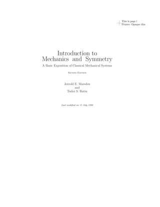
1.4 The Heavy Top
The equations of motion for a rigid body with a fixed point in a grav-
itational field provide another interesting example of a system which is
Hamiltonian relative to a Lie–Poisson bracket. See Figure 1.4.1.
The underlying Lie algebra consists of the algebra of infinitesimal Eu-
clidean motions in R3 . (These do not arise as Euclidean motions of the
body since the body has a fixed point). As we shall see, there is a close
parallel with the Poisson structure for compressible fluids.
The basic phase space we start with is again T ∗ SO(3), coordinatized by
Euler angles and their conjugate momenta. In these variables, the equations
are in canonical Hamiltonian form; however, the presence of gravity breaks
the symmetry and the system is no longer SO(3) invariant, so it cannot
be written entirely in terms of the body angular momentum Π. One also
needs to keep track of Γ, the “direction of gravity” as seen from the body.
This is defibed by Γ = A−1 k, where k points upward and A is the element
of SO(3) describing the current configuration of the body. The equations
of motion are
˙ I2 − I3
Π1 = Π2 Π3 + M gl(Γ2 χ3 − Γ3 χ2 ),
I2 I3
˙ I3 − I1
Π2 = Π3 Π1 + M gl(Γ3 χ1 − Γ1 χ3 ), (1.4.1)
I3 I1
˙ I1 − I2
Π3 = Π1 Π2 + M gl(Γ1 χ2 − Γ2 χ1 )
I1 I2
........................... 15 July 1998—18h02 ...........................
31. 1.4 The Heavy Top 17
Ω
M = total mass
g = gravitational acceleration center of mass
Ω = body angular velocity of top
l = distance from fixed point
to center of mass
lAχ
g
fixed point
k
Γ
Figure 1.4.1. Heavy top
and
˙
Γ=Γ×Ω (1.4.2)
where M is the body’s mass, g is the acceleration of gravity, χ is the body
fixed unit vector on the line segment connecting the fixed point with the
body’s center of mass, and l is the length of this segment. See Figure 1.4.1.
The Lie algebra of the Euclidean group is se(3) = R3 × R3 with the Lie
bracket
[(ξ, u), (η, v)] = (ξ × η, ξ × v − η × u). (1.4.3)
We identify the dual space with pairs (Π, Γ); the corresponding (−) Lie–
Poisson bracket, called the heavy top bracket, is
{F, G}(Π, Γ) = −Π · ( ΠF × Π G)
−Γ·( ΠF × ΓG − ΠG × Γ F ). (1.4.4)
The above equations for Π, Γ can be checked to be equivalent to
˙
F = {F, H}, (1.4.5)
where the heavy top Hamiltonian
1 Π2 Π2 Π2
H(Π, Γ) = 1
+ 2+ 3 + M glΓ · χ (1.4.6)
2 I1 I2 I3
........................... 15 July 1998—18h02 ...........................
32. 18 1. Introduction and Overview
is the total energy of the body (Sudarshan and Mukunda [1974]).
The Lie algebra of the Euclidean group has a structure which is a special
case of what is called a semidirect product. Here it is the product of the
group of rotations with the translation group. It turns out that semidirect
products occur under rather general circumstances when the symmetry in
T ∗ G is broken. In particular, notice the similarities in structure between
the Poisson bracket (1.6.16) for compressible flow and (1.4.4). For com-
pressible flow it is the density which prevents a full Diff(Ω) invariance;
the Hamiltonian is only invariant under those diffeomorphisms that pre-
serve the density. The general theory for semidirect products was developed
by Sudarshan and Mukunda [1974], Ratiu [1980, 1981, 1982], Guillemin
and Sternberg [1982], Marsden, Weinstein, Ratiu, Schmid, and Spencer
[1983], Marsden, Ratiu, and Weinstein [1984a,b], and Holm and Kupersh-
midt [1983]. The Lagrangian approach to this and related problems is given
in Holm, Marsden, and Ratiu [1998].
Exercises
˙
1.4-1. Verify that F = {F, H} are equivalent to the heavy top equations
using the heavy top Hamiltonian and bracket.
1.4-2. Work out the Euler–Poincar´ equations on se(3). Show that with
e
L(Ω, Γ) = 1 (I1 Ω2 + I2 Ω2 + I3 Ω2 ) − M glΓ · χ, the Euler–Poincar´ equations
2 1 2 3 e
are not the heavy top equations.
1.5 Incompressible Fluids
Arnold [1966a, 1969] showed that the Euler equations for an incompressible
fluid could be given a Lagrangian and Hamiltonian description similar to
that for the rigid body. His approach5 has the appealing feature that one
sets things up just the way Lagrange and Hamilton would have done: one
begins with a configuration space Q, forms a Lagrangian L on the velocity
phase space T Q and then H on the momentum phase space T ∗ Q, just as
was outlined in §1.1. Thus, one automatically has variational principles,
etc. For ideal fluids, Q = G is the group Diff vol (Ω) of volume preserving
transformations of the fluid container (a region Ω in R2 or R3 , or a Rieman-
nian manifold in general, possibly with boundary). Group multiplication
in G is composition.
Kinematics of a Fluid. The reason we select G = Diff vol (Ω) as the
configuration space is similar to that for the rigid body; namely, each ϕ
5 Arnold’s approach is consistent with what appears in the thesis of Ehrenfest from
around 1904; see Klein [1970]. However, Ehrenfest bases his principles on the more
sophisticated curvature principles of Gauss and Hertz.
........................... 15 July 1998—18h02 ...........................
33. 1.5 Incompressible Fluids 19
in G is a mapping of Ω to Ω which takes a reference point X ∈ Ω to a
current point x = ϕ(X) ∈ Ω; thus, knowing ϕ tells us where each particle
of fluid goes and hence gives us the fluid configuration. We ask that ϕ
be a diffeomorphism to exclude discontinuities, cavitation, and fluid inter-
penetration, and we ask that ϕ be volume preserving to correspond to the
assumption of incompressibility.
A motion of a fluid is a family of time-dependent elements of G, which
we write as x = ϕ(X, t). The material velocity field is defined by
∂ϕ(X, t)
V(X, t) = ,
∂t
and the spatial velocity field is defined by v(x, t) = V(X, t), where x and
X are related by x = ϕ(X, t). If we suppress “t” and write ϕ for V, note
˙
that
v = ϕ ◦ ϕ−1
˙ i.e., vt = Vt ◦ ϕ−1 ,
t (1.5.1)
where ϕt (x) = ϕ(X, t). See Figure 1.5.1.
trajectory of fluid particle
D u(x,t)
Figure 1.5.1.
We can regard (1.5.1) as a map from the space of (ϕ, ϕ) (material or La-
˙
grangian description) to the space of v’s (spatial or Eulerian description).
Like the rigid body, the material to spatial map (1.5.1) takes the canonical
bracket to a Lie–Poisson bracket; one of our goals is to understand this re-
duction. Notice that if we replace ϕ by ϕ ◦ η for a fixed (time-independent)
η ∈ Diff vol (Ω), then ϕ ◦ ϕ−1 is independent of η; this reflects the right
˙
invariance of the Eulerian description (v is invariant under composition of
ϕ by η on the right). This is also called the particle relabeling symme-
try of fluid dynamics. The spaces T G and T ∗ G represent the Lagrangian
(material) description and we pass to the Eulerian (spatial) description by
right translations and use the (+) Lie–Poisson bracket. One of the things we
want to do later is to better understand the reason for the switch between
right and left in going from the rigid body to fluids.
........................... 15 July 1998—18h02 ...........................
34. 20 1. Introduction and Overview
Dynamics of a Fluid. The Euler equations for an ideal, incompress-
ible, homogeneous fluid moving in the region Ω are
∂v
+ (v · )v = − p (1.5.2)
∂t
with the constraint div v = 0 and the boundary conditions: v is tangent
to the boundary, ∂Ω.
The pressure p is determined implicitly by the divergence-free (volume
preserving) constraint div v = 0. (See Chorin and Marsden [1993] for basic
information on the derivation of Euler’s equations.) The associated Lie al-
gebra g is the space of all divergence-free vector fields tangent to the bound-
ary. This Lie algebra is endowed with the negative Jacobi–Lie bracket of
vector fields given by
n
∂v i ∂wi
[v, w]i =
L wj − vj j . (1.5.3)
j=1
∂xj ∂x
(The sub L on [· , ·] refers to the fact that it is the left Lie algebra bracket
on g. The most common convention for the Jacobi–Lie bracket of vector
fields, also the one we adopt, has the opposite sign.) We identify g and g∗
using the pairing
v, w = v · w d3 x. (1.5.4)
Ω
Hamiltonian Structure. Introduce the (+) Lie–Poisson bracket, called
the ideal fluid bracket, on functions of v by
δF δG
{F, G}(v) = v· , d3 x, (1.5.5)
Ω δv δv L
where δF/δv is defined by
1 δF
lim [F (v + εδv) − F (v)] = δv · d3 x. (1.5.6)
ε→0ε Ω δv
With the energy function chosen to be the kinetic energy,
1 2
H(v) = v d3 x, (1.5.7)
2 Ω
one can verify that the Euler equations (1.5.2) are equivalent to the Poisson
bracket equations
˙
F = {F, H} (1.5.8)
........................... 15 July 1998—18h02 ...........................
35. 1.5 Incompressible Fluids 21
for all functions F on g. For this, one uses the orthogonal decomposition
w = Pw + p of a vector field w into a divergence-free part Pw in g and
a gradient. The Euler equations can be written
∂v
+ P(v · v) = 0. (1.5.9)
∂t
One can express the Hamiltonian structure in terms of the vorticity as a
basic dynamic variable, and show that the preservation of coadjoint orbits
amounts to Kelvin’s circulation theorem. Marsden and Weinstein [1983]
show that the Hamiltonian structure in terms of Clebsch potentials fits
naturally into this Lie–Poisson scheme, and that Kirchhoff’s Hamiltonian
description of point vortex dynamics, vortex filaments, and vortex patches
can be derived in a natural way from the Hamiltonian structure described
above.
Lagrangian Structure. The general framework of the Euler-Poincar´ e
and the Lie–Poisson equations gives other insights as well. For example,
this general theory shows that the Euler equations are derivable from the
“variational principle”
b
1 2
δ v d3 x = 0
a Ω 2
which is to hold for all variations δv of the form
˙
δv = u + [v, u]L
(sometimes called Lin constraints) where u is a vector field (represent-
ing the infinitesimal particle displacement) vanishing at the temporal end-
points6 .
There are important functional analytic differences between working in
material representation (that is, on T ∗ G) and in Eulerian representation,
that is, on g∗ that are important for proving existence and uniqueness theo-
rems, theorems on the limit of zero viscosity, and the convergence of numer-
ical algorithms (see Ebin and Marsden [1970], Marsden, Ebin, and Fischer
[1972], and Chorin, Hughes, Marsden, and McCracken [1978]). Finally, we
note that for two-dimensional flow , a collection of Casimir functions is
given by
C(ω) = Φ(ω(x)) d2 x (1.5.10)
Ω
for Φ : R → R any (smooth) function where ωk = × v is the vorticity .
For three-dimensional flow, (1.5.10) is no longer a Casimir.
6 As mentioned earlier, this form of the variational (strictly speaking a Lagrange
d’Alembert type) principle is due to Newcomb [1962]; see also Bretherton [1970]. For
the case of general Lie algebras, it is due to Marsden and Scheurle [1993b]; see also Bloch,
Krishnaprasad, Marsden and Ratiu [1994b]. See also the review article of Morrison [1994]
for a somewhat different perspective.
........................... 15 July 1998—18h02 ...........................
36. 22 1. Introduction and Overview
Exercises
1.5-1. Show that any divergence-free vector field X on R3 can be written
globally as a curl of another vector field and, away from equilibrium points,
can locally be written as
X = f × g,
where f and g are real-valued functions on R3 . Assume this (so-called
Clebsch-Monge) representation also holds globally. Show that the particles
of fluid, which follow trajectories satisfying x = X(x), are trajectories of a
˙
Hamiltonian system with a bracket in the form of Exercise 1.3-2.
1.6 The Maxwell–Vlasov System
Plasma physics provides another beautiful application area for the tech-
niques discussed in the preceding sections. We shall briefly indicate these
in this section. The period 1970–1980 saw the development of noncanonical
Hamiltonian structures for the Korteweg-de Vries (KdV) equation (due to
Gardner, Kruskal, Miura, and others; see Gardner [1971]) and other soliton
equations. This quickly became entangled with the attempts to understand
integrability of Hamiltonian systems and the development of the algebraic
approach; see, for example, Gelfand and Dorfman [1979], Manin [1979]
and references therein. More recently these approaches have come together
again; see, for instance, Reyman and Semenov–Tian-Shansky [1990], Moser
and Veselov [19–]. KdV type models are usually derived from or are approx-
imations to more fundamental fluid models and it seems fair to say that the
reasons for their complete integrability are not yet completely understood.
Some History. For fluid and plasma systems, some of the key early
works on Poisson bracket structures were Dashen and Sharp [1968], Goldin
[1971], Iwinski and Turski [1976], Dzyaloshinski and Volovick [1980], Mor-
rison and Greene [1980], and Morrison [1980]. In Sudarshan and Mukunda
[1974], Guillemin and Sternberg [1982], and Ratiu [1980, 1982], a general
theory for Lie–Poisson structures for special kinds of Lie algebras, called
semidirect products, was begun. This was quickly recognized (see, for ex-
ample, Marsden [1982], Marsden, Weinstein, Ratiu, Schmid, and Spencer
[1983], Holm and Kuperschmidt [1983], and Marsden, Ratiu and Weinstein
[1984a,b]) to be relevant to the brackets for compressible flow; see §1.7
below.
Derivation of Poisson Structures. A rational scheme for systemati-
cally deriving brackets is needed, since, for one thing, a direct verification
of Jacobi’s identity can be inefficient and time-consuming. (See Morrison
[1982] and Morrison and Weinstein [1982].) Here we outline a derivation of
the Maxwell–Vlasov bracket by Marsden and Weinstein [1982]. The method
is similar to Arnold’s, namely by performing a reduction starting with:
........................... 15 July 1998—18h02 ...........................
37. 1.6 The Maxwell–Vlasov System 23
(i) canonical brackets in a material representation for the plasma; and
(ii) a potential representation for the electromagnetic field.
One then identifies the symmetry group and carries out reduction by this
group in a manner similar to that we desribed for Lie–Poisson systems.
For plasmas, the physically correct material description is actually slightly
more complicated; we refer to Cendra, Holm, Hoyle, and Marsden [1998]
for a full account.
Parallel developments can be given for many other brackets, such as the
charged fluid bracket by Spencer and Kaufman [1982]. Another method,
based primarily on Clebsch potentials, was developed in a series of papers
by Holm and Kupershmidt (for example, [1983]) and applied to a number
of interesting systems, including superfluids and superconductors. They
also pointed out that semidirect products were appropriate for the MHD
bracket of Morrison and Greene [1980].
The Maxwell–Vlasov System. The Maxwell–Vlasov equations for a
collisionless plasma are the fundamental equations in plasma physics7 . In
Euclidean space, the basic dynamical variables are:
f (x, v, t) : the plasma particle number density per phase space;
volume d3 x d3 v;
E(x, t) : the electric field;
B(x, t) : the magnetic field.
The equations for a collisionless plasma for the case of a single species
of particles with mass m and charge e are
∂f ∂f e 1 ∂f
+v· + E+ v×B · = 0,
∂t ∂x m c ∂v
1 ∂B
= −curl E,
c ∂t (1.6.1)
1 ∂E 1
= curl B − jf ,
c ∂t c
div E = ρf and div B = 0.
The current defined by f is given by
jf = e vf (x, v, t) d3 v
and the charge density by
ρf = e f (x, v, t) d3 v.
7 See, for example, Clemmow and Dougherty [1959], Van Kampen and Felderhof
[1967], Krall and Trivelpiece [1973], Davidson [1972], Ichimaru [1973], and Chen [1974].
........................... 15 July 1998—18h02 ...........................
38. 24 1. Introduction and Overview
Also, ∂f /∂x and ∂f /∂v denote the gradients of f with respect to x and
v, respectively, and c is the speed of light. The evolution equation for f
results from the Lorentz force law and standard transport assumptions.
The remaining equations are the standard Maxwell equations with charge
density ρf and current jf produced by the plasma.
Two limiting cases will aid our discussions. First, if the plasma is con-
strained to be static, that is, f is concentrated at v = 0 and t-independent,
we get the charge-driven Maxwell equations:
1 ∂B
= −curl E,
c ∂t
1 ∂E (1.6.2)
= curl B,
c ∂t
div E = ρ and div B = 0.
Second, if we let c → ∞, electrodynamics becomes electrostatics, and we
get the Poisson-Vlasov equation:
∂f ∂f e ∂ϕf ∂f
+v· − · = 0, (1.6.3)
∂t ∂x m ∂x ∂v
where – 2 ϕf = ρf . In this context, the name “Poisson-Vlasov” seems quite
appropriate. The equation is, however, formally the same as the earlier
Jeans [1919] equation of stellar dynamics. H´non [1982] has proposed calling
e
it the “collisionless Boltzmann equation.”
Maxwell’s equations. For simplicity, we let m = e = c = 1. As the basic
configuration space, we take the space A of vector potentials A on R3 (for
the Yang–Mills equations this is generalized to the space of connections
on a principal bundle over space). The corresponding phase space T ∗ A is
identified with the set of pairs (A, Y), where Y is also a vector field on R3 .
The canonical Poisson bracket is used on T ∗ A :
δF δG δF δG
{F, G} = − d3 x. (1.6.4)
δA δY δY δA
The electric field is E = −Y and the magnetic field is B = curl A.
With the Hamiltonian
1 2
H(A, Y) = ( E + B 2 ) d3 x, (1.6.5)
2
Hamilton’s canonical field equations (1.1.14) are checked to give the equa-
tions for ∂E/∂t and ∂A/∂t which imply the vacuum Maxwell’s equations.
Alternatively, one can begin with T A and the Lagrangian
˙ 1 ˙
L(A, A) = A 2
− ×A 2
d3 x (1.6.6)
2
........................... 15 July 1998—18h02 ...........................
39. 1.6 The Maxwell–Vlasov System 25
and use the Euler–Lagrange equations and variational principles.
It is of interest to incorporate the equation div E = ρ and, correspond-
ingly, to use directly the field strengths E and B, rather than E and A. To
do this, we introduce the gauge group G, the additive group of real-valued
functions ψ : R3 → R. Each ψ ∈ G transforms the fields according to the
rule
(A, E) → (A + ψ, E). (1.6.7)
Each such transformation leaves the Hamiltonian H invariant and is a
canonical transformation, that is, it leaves Poisson brackets intact. In this
situation, as above, there will be a corresponding conserved quantity, or
momentum map in the same sense as in §1.3. As mentioned there, some
simple general formulas for computing them will be studied in detail in
Chapter 12. For the action (1.6.7) of G on T ∗ A, the associated momentum
map is
J(A, Y) = div E, (1.6.8)
so we recover the fact that div E is preserved by Maxwell’s equations (this
is easy to verify directly using div curl = 0). Thus we see that we can
incorporate the equation div E = ρ by restricting our attention to the set
J−1 (ρ). The theory of reduction is a general process whereby one reduces
the dimension of a phase space by exploiting conserved quantities and sym-
metry groups. In the present case, the reduced space is J−1 (ρ)/G which is
identified with Maxρ , the space of E’s and B’s satisfying div E = ρ and
div B = 0.
The space Maxρ inherits a Poisson structure as follows. If F and K are
functions on Maxρ , we substitute E = −Y and B = × A to express F
and K as functionals of (A, Y). Then we compute the canonical brackets
on T ∗ A and express the result in terms of E and B. Carrying this out using
the chain rule gives
δF δK δK δF
{F, K} = · curl − · curl d3 x, (1.6.9)
δE δB δE δB
where δF/δE and δF/δB are vector fields, with δF/δB divergence-free.
These are defined in the usual way; for example,
1 δF
lim [F (E + εδE, B) − F (E, B)] = · δE d3 x. (1.6.10)
ε→0ε δE
This bracket makes Maxρ into a Poisson manifold and the map (A, Y) →
(−Y, × A) into a Poisson map. The bracket (1.6.9) was discovered (by
a different procedure) by Pauli [1933] and Born and Infeld [1935]. We refer
to (1.6.9) as the Pauli-Born-Infeld bracket or the Maxwell–Poisson
bracket for Maxwell’s equations.
........................... 15 July 1998—18h02 ...........................
40. 26 1. Introduction and Overview
With the energy H given by (1.6.5) regarded as a function of E and B,
˙
Hamilton’s equations in bracket form F = {F, H} on Maxρ captures the
full set of Maxwell’s equations (with external charge density ρ).
The Poisson-Vlasov Equation. Morrison [1980] showed that the Poisson-
Vlasov equations form a Hamiltonian system with
1 1
H(f ) = v 2 f (x, v, t) d3 x d3 v + ϕf 2
d3 x (1.6.11)
2 2
and the Poisson-Vlasov bracket
δF δG
{F, G} = f , d3 x d3 v, (1.6.12)
δf δf xv
where { , }xv is the canonical bracket on (x, v)-space. As was observed in
Gibbons [1981] and Marsden and Weinstein [1982], this is the (+) Lie–
Poisson bracket associated with the Lie algebra g of functions of (x, v)
with Lie bracket the canonical Poisson bracket.
According to the general theory, this Lie–Poisson structure is obtained by
reduction from canonical brackets on the cotangent bundle of the group un-
derlying g, just as was the case for the rigid body and incompressible fluids.
This time the group G = Diff can is the group of canonical transformations
of (x, v)-space. The Poisson-Vlasov equations can equally well be written
in canonical form on T ∗ G. This is the Lagrangian description of a plasma,
and the Hamiltonian description here goes back to Low [1958], Katz [1961],
and Lundgren [1963]. Thus, one can start with the Lagrangian description
with canonical brackets and, through reduction, derive the brackets here.
There are other approaches to the Hamiltonian formulation using analogs
of Clebsch potentials; see, for instance, Su [1961], Zakharov [1971], and
Gibbons, Holm, and Kupershmidt [1982]. See Cendra, Holm, Hoyle, and
Marsden [1998] for further information on these topics.
The Poisson-Vlaslov to Compressible Flow Map. Before going on
to the Maxwell–Vlasov equations, we point out a remarkable connection be-
tween the Poisson-Vlasov bracket (1.6.12) and the bracket for compressible
flow.
The Euler equations for compressible flow in a region Ω in R3 are
∂v
ρ + (v · )v =− p (1.6.13)
∂t
and
∂ρ
+ div(ρv) = 0, (1.6.14)
∂t
with the boundary condition
v tangent to ∂Ω.
........................... 15 July 1998—18h02 ...........................