


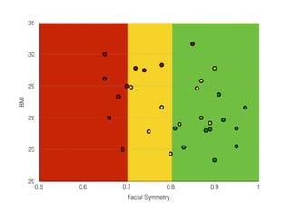
![Symmetry >.8
samples = 30
count = [10, 10, 10]
[att, ave, un]](https://image.slidesharecdn.com/introductiontomachinelearningalgorithms-180312021825/85/Introduction-to-machine-learning-algorithms-83-320.jpg)
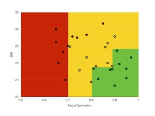
![Symmetry >.8
samples = 30
count = [10, 10, 10]
BMI < 25
samples = 17
count = [10, 5, 2]
BMI < 24
samples = 13
count = [0, 5, 8]
true false
[att, ave, un]](https://image.slidesharecdn.com/introductiontomachinelearningalgorithms-180312021825/85/Introduction-to-machine-learning-algorithms-84-320.jpg)
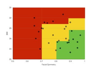
![Symmetry >.8
samples = 30
count = [10, 10, 10]
BMI < 25
samples = 17
count = [10, 5, 2]
BMI < 24
samples = 13
count = [0, 5, 8]
Well-Groomed=1
samples = 12
count = [9, 3, 0]
Well-Groomed=1
samples =5
count = [1, 2, 2]
true false
[att, ave, un]](https://image.slidesharecdn.com/introductiontomachinelearningalgorithms-180312021825/85/Introduction-to-machine-learning-algorithms-85-320.jpg)
![Symmetry >.8
samples = 30
count = [10, 10, 10]
BMI < 25
samples = 17
count = [10, 5, 2]
BMI < 24
samples = 13
count = [0, 5, 8]
Well-Groomed=1
samples = 12
count = [9, 3, 0]
Well-Groomed=1
samples =5
count = [1, 2, 2]
samples = 6
count = [6, 0, 0]
class = attractive
Hip-to-Waist >.84
samples = 6
count = [3, 3, 0]
Hip-to-Waist >.79
samples = 3
count = [1, 2, 0]
samples = 2
count = [0, 0, 2]
class = unattractive
true false
[att, ave, un]](https://image.slidesharecdn.com/introductiontomachinelearningalgorithms-180312021825/85/Introduction-to-machine-learning-algorithms-86-320.jpg)
![Symmetry >.8
samples = 30
count = [10, 10, 10]
BMI < 25
samples = 17
count = [10, 5, 2]
BMI < 24
samples = 13
count = [0, 5, 8]
Well-Groomed=1
samples = 12
count = [9, 3, 0]
Well-Groomed=1
samples =5
count = [1, 2, 2]
samples = 6
count = [6, 0, 0]
class = attractive
Hip-to-Waist >.84
samples = 6
count = [3, 3, 0]
Hip-to-Waist >.79
samples = 3
count = [1, 2, 0]
samples = 3
count = [3, 0, 0]
class = attractive
samples = 3
count = [0, 3, 0]
class = average
samples = 1
count = [1, 0, 0]
class = attractive
samples = 2
count = [0, 2, 0]
class = average
samples = 2
count = [0, 0, 2]
class = unattractive
true false
[att, ave, un]](https://image.slidesharecdn.com/introductiontomachinelearningalgorithms-180312021825/85/Introduction-to-machine-learning-algorithms-87-320.jpg)

![Euclidean Distance
point a = [a1, a2]
point b = [b1, b2]](https://image.slidesharecdn.com/introductiontomachinelearningalgorithms-180312021825/85/Introduction-to-machine-learning-algorithms-93-320.jpg)
![Euclidean Distance
point a = [a1, a2]
point b = [b1, b2]
Two dimensions (features)](https://image.slidesharecdn.com/introductiontomachinelearningalgorithms-180312021825/85/Introduction-to-machine-learning-algorithms-94-320.jpg)
![Euclidean Distance
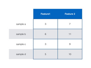
a = [3, 7]
b = [6, 11]
Feature Vector](https://image.slidesharecdn.com/introductiontomachinelearningalgorithms-180312021825/85/Introduction-to-machine-learning-algorithms-96-320.jpg)
![Euclidean Distance
a = [3, 7]
b = [6, 11]
Feature Vector](https://image.slidesharecdn.com/introductiontomachinelearningalgorithms-180312021825/85/Introduction-to-machine-learning-algorithms-97-320.jpg)
![Euclidean Distance
a = [3, 7]
b = [6, 11]
Feature Vector](https://image.slidesharecdn.com/introductiontomachinelearningalgorithms-180312021825/85/Introduction-to-machine-learning-algorithms-98-320.jpg)
![Euclidean Distance
a = [3, 7]
b = [6, 11]
Feature Vector](https://image.slidesharecdn.com/introductiontomachinelearningalgorithms-180312021825/85/Introduction-to-machine-learning-algorithms-99-320.jpg)
![Euclidean Distance
a = [3, 7]
b = [6, 11]
Feature Vector
Distance between points (vectors) a and b:](https://image.slidesharecdn.com/introductiontomachinelearningalgorithms-180312021825/85/Introduction-to-machine-learning-algorithms-100-320.jpg)
![X2
0
3
6
9
12
15
X1
0 3 6 9 12 15
Euclidean Distance
b = [6, 11]
Distance between points (vectors) a and b:
a = [3, 7]](https://image.slidesharecdn.com/introductiontomachinelearningalgorithms-180312021825/85/Introduction-to-machine-learning-algorithms-101-320.jpg)
![X2
0
3
6
9
12
15
X1
0 3 6 9 12 15
Euclidean Distance
b = [6, 11]
Distance between points (vectors) a and b:
32
a = [3, 7]
3](https://image.slidesharecdn.com/introductiontomachinelearningalgorithms-180312021825/85/Introduction-to-machine-learning-algorithms-102-320.jpg)
![X2
0
3
6
9
12
15
X1
0 3 6 9 12 15
Euclidean Distance
a = [3, 7]
b = [6, 11]
Distance between points (vectors) a and b:
32 + 42
3
4](https://image.slidesharecdn.com/introductiontomachinelearningalgorithms-180312021825/85/Introduction-to-machine-learning-algorithms-103-320.jpg)
![X2
0
3
6
9
12
15
X1
0 3 6 9 12 15
Euclidean Distance
a = [3, 7]
b = [6, 11]
Distance between points (vectors) a and b:
32 + 42 = squared distance
3
4](https://image.slidesharecdn.com/introductiontomachinelearningalgorithms-180312021825/85/Introduction-to-machine-learning-algorithms-104-320.jpg)
![X2
0
3
6
9
12
15
X1
0 3 6 9 12 15
Euclidean Distance
a = [3, 7]
b = [6, 11]
Distance between points (vectors) a and b:
32 + 42 = squared distance
3
4
sqrt(9 + 16)](https://image.slidesharecdn.com/introductiontomachinelearningalgorithms-180312021825/85/Introduction-to-machine-learning-algorithms-105-320.jpg)
![X2
0
3
6
9
12
15
X1
0 3 6 9 12 15
Euclidean Distance
a = [3, 7]
b = [6, 11]
Distance between points (vectors) a and b:
32 + 42 = squared distance
3
4
sqrt(9 + 16)
sqrt(25) = 5
5distance =](https://image.slidesharecdn.com/introductiontomachinelearningalgorithms-180312021825/85/Introduction-to-machine-learning-algorithms-106-320.jpg)


![[ [216, 203, 125, 10, 84, 241, 149, 159, 212, 118, 135, 158, 11, 91, 36, 177, 176, 253, 132, 210, 159, 20, 153, 131, 132, 55,16, 132],
[184, 34, 95, 225, 60, 218, 49, 193, 93, 119, 68, 133, 195,104, 248, 18, 18, 136, 90, 71, 81, 41, 233, 53, 46, 87,86, 243],
[ 85, 61, 220, 170, 206, 34, 141, 97, 66, 217, 124, 143, 241,205, 76, 123, 66, 72, 231, 116, 244, 74, 155, 144, 47, 230,171, 165],
[156, 87, 181, 90, 160, 2, 184, 112, 108, 62, 223, 153, 93, 244, 83, 187, 83, 18, 134, 28, 121, 244, 202, 176, 228, 233,76, 13],
[ 76, 238, 128, 183, 119, 130, 34, 12, 112, 254, 90, 167, 64,89, 170, 221, 196, 69, 82, 11, 65, 86, 254, 111, 134, 0,148, 246],
[105, 178, 254, 31, 32, 133, 57, 40, 6, 85, 115, 56, 132,84, 35, 119, 158, 182, 106, 77, 84, 106, 164, 230, 54, 42,55, 130],
[ 25, 86, 222, 59, 242, 111, 59, 183, 236, 214, 251, 7, 142,90, 179, 80, 163, 159, 26, 143, 108, 109, 229, 223, 220, 196,21, 18],
[ 21, 42, 109, 188, 91, 93, 246, 236, 125, 48, 151, 12, 178,26, 118, 135, 77, 84, 179, 208, 114, 224, 99, 246, 68, 21, 69, 39],
[253, 66, 78, 55, 39, 107, 248, 90, 124, 107, 51, 92, 150,234, 91, 177, 146, 80, 8, 179, 148, 229, 233, 59, 164, 199,252, 43],
[ 79, 60, 5, 70, 37, 218, 19, 9, 90, 74, 198, 129, 61,160, 206, 11, 37, 171, 44, 241, 228, 190, 232, 99, 7, 100, 83, 225],
[211, 38, 52, 167, 206, 139, 215, 209, 202, 102, 122, 77, 86,117, 134, 22, 176, 94, 22, 201, 6, 73, 156, 226, 36, 0,50, 119],
[159, 24, 197, 215, 16, 243, 177, 13, 108, 211, 6, 97, 75,214, 121, 92, 154, 109, 213, 163, 123, 20, 190, 174, 89, 6,136, 164],
[183, 136, 245, 175, 233, 62, 141, 117, 150, 74, 182, 175, 36,230, 93, 109, 212, 43, 10, 75, 234, 124, 70, 244, 161, 76,241, 223],
[150, 7, 184, 20, 133, 22, 112, 212, 48, 30, 156, 113, 127,207, 219, 173, 223, 127, 202, 172, 39, 98, 134, 124, 130, 34,210, 101],
[101, 77, 87, 37, 152, 112, 34, 106, 30, 23, 79, 214, 245,152, 129, 243, 109, 213, 170, 190, 220, 25, 76, 205, 135, 227,225, 165],
[108, 184, 172, 121, 8, 83, 106, 116, 235, 55, 73, 204, 50,40, 124, 153, 225, 157, 13, 28, 105, 62, 242, 214, 56, 159,137, 67],
[ 14, 75, 26, 47, 74, 205, 45, 219, 27, 18, 79, 28, 49,224, 85, 214, 180, 105, 183, 87, 18, 64, 7, 61, 125, 87,38, 98],
[122, 146, 4, 72, 150, 249, 77, 90, 6, 132, 134, 151, 164,29, 94, 188, 251, 177, 0, 206, 193, 182, 231, 43, 32, 32,80, 147],
[ 26, 39, 76, 12, 35, 81, 103, 233, 204, 138, 82, 28, 5,68, 229, 197, 52, 215, 224, 117, 101, 4, 154, 4, 205, 50,251, 114],
[ 68, 176, 23, 246, 11, 57, 62, 25, 38, 17, 136, 106, 113,140, 254, 43, 231, 150, 12, 114, 77, 8, 214, 187, 92, 66,195, 70],
[ 20, 241, 148, 151, 37, 4, 14, 231, 225, 53, 232, 240, 223,59, 234, 134, 247, 242, 212, 63, 201, 38, 63, 200, 128, 139,167, 173],
[ 60, 244, 33, 111, 143, 127, 168, 237, 189, 63, 125, 181, 92,91, 14, 211, 21, 26, 253, 109, 174, 100, 138, 138, 221, 204,29, 230],
[ 81, 174, 217, 93, 65, 134, 7, 36, 176, 122, 226, 23, 223,28, 202, 5, 54, 205, 169, 14, 88, 178, 84, 198, 96, 201,230, 193],
[215, 168, 125, 92, 70, 151, 183, 210, 36, 32, 19, 51, 42,64, 19, 146, 183, 246, 0, 184, 236, 7, 226, 118, 113, 241, 85, 89],
[ 31, 158, 210, 16, 199, 58, 224, 7, 203, 86, 103, 45, 28,54, 92, 204, 243, 117, 75, 208, 248, 223, 87, 250, 14, 43,102, 66],
[ 13, 236, 138, 67, 236, 109, 113, 46, 115, 19, 214, 154, 199,248, 55, 172, 214, 249, 125, 154, 139, 141, 188, 78, 107, 200, 196, 16],
[ 65, 150, 158, 254, 114, 177, 120, 15, 65, 58, 79, 171, 118,32, 250, 81, 27, 85, 128, 146, 144, 234, 139, 26, 6, 68,133, 205],
[123, 68, 216, 34, 139, 34, 34, 175, 213, 72, 76, 19, 32,138, 132, 111, 242, 249, 177, 89, 61, 72, 252, 79, 20, 171,174, 177] ]](https://image.slidesharecdn.com/introductiontomachinelearningalgorithms-180312021825/85/Introduction-to-machine-learning-algorithms-157-320.jpg)
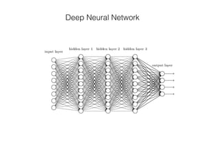


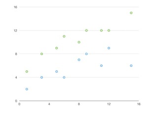
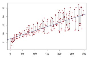
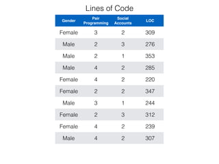
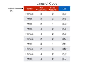
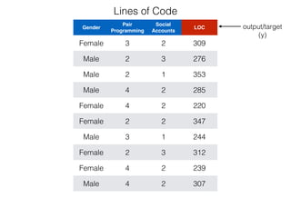
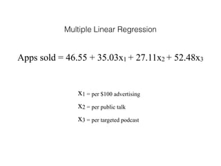
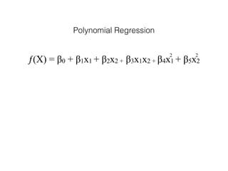
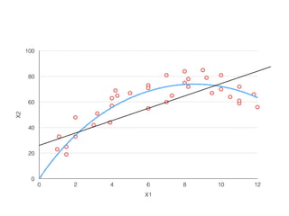
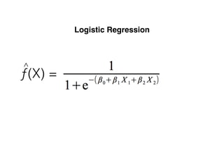
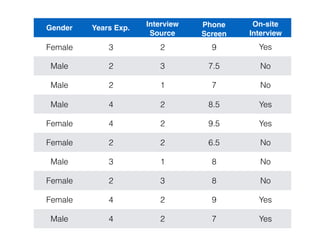
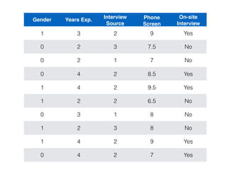
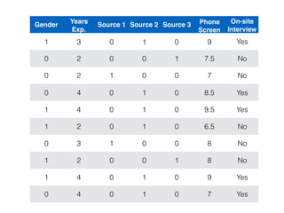
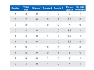
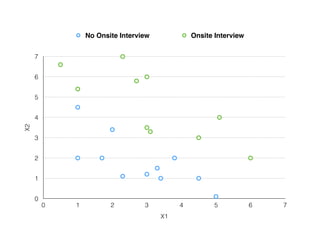
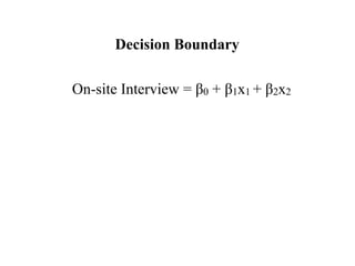
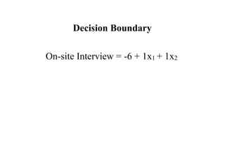
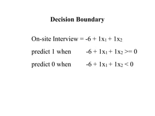
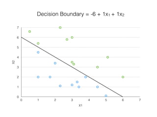
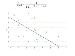
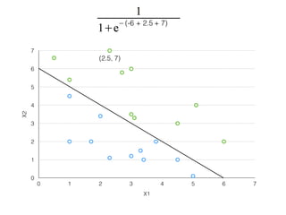
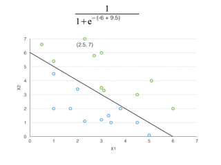
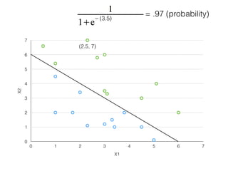
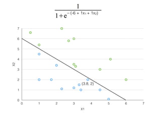
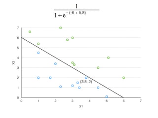
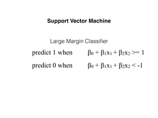
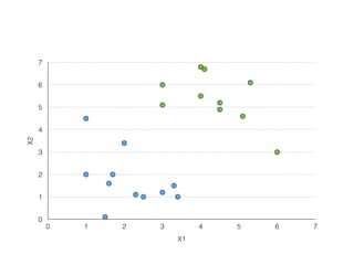
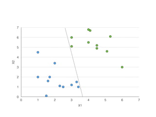
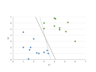
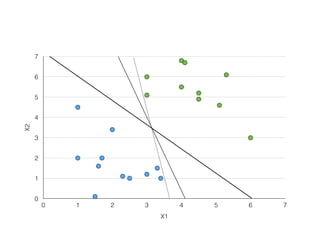
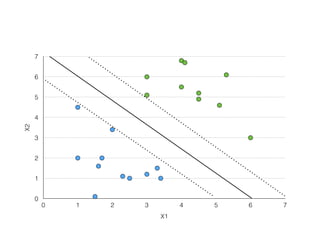
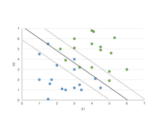
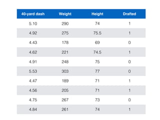
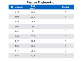
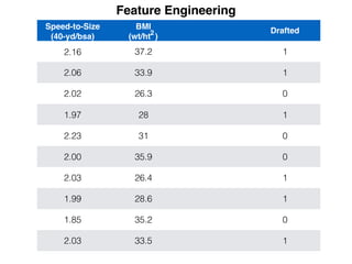
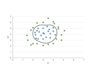
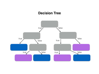
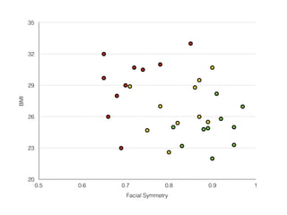
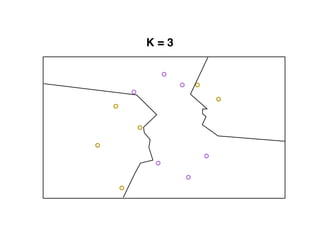
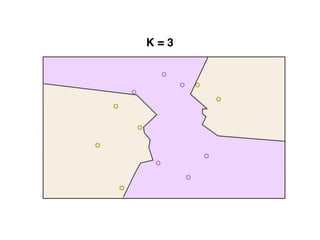
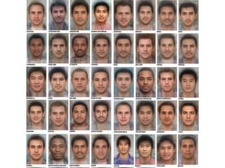
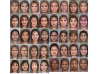
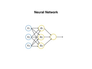
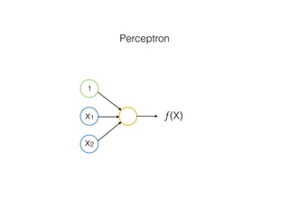
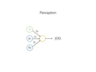
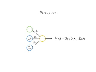
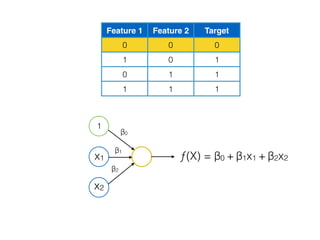
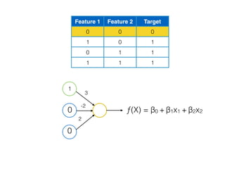
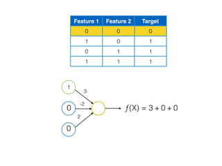
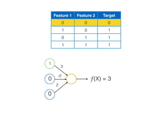
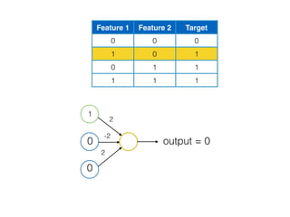
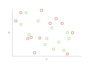
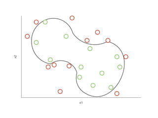
The document provides an overview of various machine learning techniques including linear regression, logistic regression, support vector machine, decision tree, and k-nearest neighbor. It explains concepts such as equation representations, predictions, feature engineering, classification methods, and model evaluation. Additionally, it discusses data examples involving social factors, programming patterns, and classifications based on gender and interview experiences.


![제 23회 보아즈(BOAZ) 빅데이터 컨퍼런스 - [MBOAX] : ABSA를 활용한 소비자 반응 분석 기반 운영 효율화 대시보드 설계](https://cdn.slidesharecdn.com/ss_thumbnails/3-1boaz23rdconferencemboax-260203102709-9d519923-thumbnail.jpg?width=640&height=640&fit=bounds)

![7.__Developing_a_Research_Proposal[1].pptx](https://cdn.slidesharecdn.com/ss_thumbnails/7-260131073037-df92dd7d-thumbnail.jpg?width=640&height=640&fit=bounds)


