FAIR (Factor Analysis of Information Risk) is a framework for measuring and analyzing information risk in a logical and quantitative way. It consists of (1) an ontology that defines the factors that contribute to risk and their relationships, (2) methods for measuring these factors, and (3) a computational model that calculates risk by simulating the relationships between measured factors. FAIR aims to provide an objective, evidence-based approach to risk analysis and avoid common pitfalls like inaccurate models, poor communication, and focus on worst-case scenarios. It measures factors like threat frequency, vulnerability, and loss magnitude on quantitative scales to determine overall risk.

1. Introduction to FAIR
(Factor Analysis of Information Risk)
by
Osama Salah

2. References
This presentation is strongly based on:
• Measuring and Managing Information Risk – A FAIR Approach
by Jack Freud and Jack Jones.
• How to measure anything in Cyber Security Risk
by Douglas W. Hubbard and Richard Seiersen
• “The Open FAIR Body of Knowledge”
• “Open FAIR Foundation” Study Guide

3. What is FAIR?
• Factor Analysis of Information Risk
• Originally published in 2005 by Jack Jones
• Adopted by the Open Group (Industry Standard)
• The Open FAIR Body of Knowledge.
• Risk Taxonomy Standard (O-RT)
• Risk Analysis Standard (O-RA)

4. What is FAIR
A well-reasoned and logical risk evaluation framework made up of:
a) An ontology of the factors that make up risk and their relationship to one
another.
b) Methods for measuring the factors that drive risk. (logical and rational)
c) A computational engine that derives risk by mathematically simulating
the relationships between measured factors (like Monte Carlo Analysis)
d) A scenario modeling construct to build and analyze risk scenarios.
FAIR focuses on Risk Analysis i.e. evaluating the significance and/or enabling
the comparison of options. It supports explaining how the analysis was
performed and what assumptions were made. Conclusions are defensible.

5. Common causes of inaccurate risk analysis
…that FAIR helps to avoid
• Broken Models, relationship between factors are not clear
• Broken communication with business
• Poorly defined scope, scenarios
• Focus on possibility vs. probability (worst case scenarios)
• Bad estimates/measurements
• Poorly defined measurement scales
• Math on ordinal scales
• Normalization of risk across domains

6. The Risk Management Stack
Cost-Effective Risk Management
Well-informed Decisions
Effective Comparisons
Meaningful Measurements
Accurate Models

7. The Problem with Heat Maps
• Tony Cox Jr., who holds a Ph.D. in risk analysis from Massachusetts Institute of
Technology, probably has studied risk matrices more than anyone else, and he
has concluded that risk matrices are often "worse than useless."
• ”As remarkable as this sounds, he argues (and demonstrates) it could even be
worse than randomly prioritized risks”.
• “…there is not a single study indicating that the use of such methods actually
helps reduce risks.”
• "…the proliferation of such methods may well be due entirely to their
perceived benefits and yet have no objective value”.
Source: Douglas Hubbard author of “How to measure Risk in Cyber Security”

8. Risk Management Humor
• Slide From the presentation of the research of P. Thomas, R. Bratvold,
and J. E. Bickel, “The Risk of Using Risk Matrices,” Society of
Petroleum Engineers Economics & Management 4, no. 2 (April 2014):
56-66

9. Quick Example and summary of issues
• We will go through these very quickly.
• All findings are backed by empirical research, they are not just
“opinions”.

10. The Range Compression Problem
Risk A: Likelihood is 2%, impact is $10 million  2% * $10 million = $200,000
Risk B: likelihood is 20%, impact $100 million  20% * $100 million = $20 million
Risk B 100 times Risk A
Source: Douglas Hubbard author of “How to measure Risk in Cyber Security”

11. The Range Compression Problem
Risk A: Likelihood is 50%, impact is $9 million  50% * $9 million = $4.5 million
Risk B: likelihood is 60%, impact $2 million  60% * $2 million = $1.2 million
Risk A > Risk B but Risk A is Medium and B is High
Source: Douglas Hubbard author of “How to measure Risk in Cyber Security”

12. Some of the Problems with Heat maps/Risk
Matrices
• The scales (buckets) are chosen arbitrary but their choice impacts the response. For example: on a scale of 1
to 5, "1" will be chosen more often than on a scale of 1-10 even if "1" is defined exactly the same”
• Interpretations vary significantly. For example "Very likely" was found to be ranging from 43% to 99%.
• Providing ordinal numbers to verbal scales or instead of them. It leads to different results, over half of the
time the additional information is ignored.
• Sometimes ordinal scales for likelihood don't even define the reference time period (Like yearly etc.).
• Direction of scale ( 5 is high or 5 is low affects response).
• Anchoring: Just thinking of a number prior to analysis impacts the choices. You think of a high number you
end up choosing higher ratings.
• Irrelevant external factors impact our response. If people are smiling you tend to accept more risk, recalling
an event causing fear (not related to the risk analysis) and you end up accepting less risk…etc.
• Other cognitive biases: Availability Heuristics, Gambler's Fallacy, Optimism Bias, Confirmation Bias, Framing,
Overconfidence…

13. Fun Reading on Cognitive Bias/Fallacies

14. Terminology - Asset
Assets: Anything that may be affected in a manner whereby its value is
diminished or the act introduces liability to the owner.
Assets are things that we value. They usually have intrinsic value, are
replaceable in some way or create potential liability.
The business cares about the “real asset”. For example a server might be an
asset but most often it isn’t the primary asset of interest in the analysis. It
may be the point of attack through which an attacker gains access to the
data.
Reputation is an important organizational asset but not in the context of risk
management. There it is an outcome of an event, for example reputation
damage due to sensitive customer information disclosure.

15. Terminology - Threat
Threat
Every action has to have an actor to carry it out. Typically called “Threat
agent” or “Threat community” but generally referred to as threats.
They need to represent an ability to actively do harm to whoever we
are performing the risk analysis (organization, person…).
A threat acts directly against the asset.
Threats must have the potential to inflict loss.

16. Terminology - Is it a threat?
Item Threat?
Advanced persistent Threat (APT)
Hacktivist
Cloud
Voice of IP
Social Engineering
Organized Crime
State sponsored attack
Social Networking
Mobile devices and applications
Distributed denial of service
Item Threat?
Advanced persistent Threat (APT) Form of Attack, Scenario
Hacktivist Yes - Person
Cloud Thing, Infrastructure, technology
Voice of IP Thing, technology
Social Engineering Form of Attack, Technique
Organized Crime Yes – Person(s)
State sponsored attack Class of threat event
Social Networking Thing, Potential method for attack
Mobile devices and applications Thing, technology, device
Distributed denial of service Form of attack

17. Terminology – Threat Communities
Threat Communities: A subset of the overall threat agent population
that shares key characteristics. Examples:
• Nation States
• Cyber Criminals
• Insiders:
• Privileged Insiders
• Non-privileged Insiders
• Hacktivists/Activists

18. Terminology – Threat Profiling
Threat Profiling (Example Nation State)
Threat profiling is the technique of building a list of common characteristics with a
given threat community.
Factor Value
Motive Nationalism
Primary Intent Data gathering or disruption of critical infrastructure in furtherance of military,
economical, or political goals.
Sponsorship State sponsored, yet often clandestine
Preferred general target characteristics Organizations/Individuals that represent assets/targets by the state sponsor
Preferred targets Entities with significant financial, commercial, intellectual property, and/or critical
infrastructure assets.
Capability Highly funded, trained, and skilled. Can bring a nearly unlimited arsenal of resources to
bear in pursuit of their goals.
Personal risk tolerance Very high, up to and including death.
Concern for Collateral Damage Some, if it interferes with the clandestine nature of the attack.

19. Probability vs. Possibility
• Possibility is “binary": something is possible or it is not.
• Probability is a continuum addressing the area between certainty and
impossibility.
Risk management deals with probability as it deals with future events that always
have some amount of uncertainty.
Probability is not prediction. The odds of rolling “1” with a single die is 1 in 6, but
we can’t predict on what the dice will fall.
Probability Possibility
There is a 50% chance of rain between 10am and 2pm today. It’s possible it could rain today.
The chances of winning the lottery are one in 14million. It’s possible to we could win the lottery.
The chance of being killed by a shark is one in 300 million. It’s possible we could be killed by a shark when swimming.

20. Accuracy and Precision
• Accuracy: The ability to provide correct information.
• Precision: The ability to be exact, as in performance, execution or
amount.
An example of an estimate that is precise but inaccurate would be to
estimate that the wingspan of a 747 is exactly 107.5’
An example of an estimate that is accurate but not precise would be to
estimate that the wingspan of a 747 is between 1’ and 1,000’.
We usually aim for accuracy with a useful amount of precision.
There are actually 3 models ranging from 195’ to 224’.

21. Measurements
• The purpose of measurement is to reduce uncertainty.
• Measurement: A quantitatively expressed reduction of uncertainty based
on one or more observations (Observations that quantitatively reduce
uncertainty.)
• It’s not about ‘perfect’, just good enough for the particular decision that
needs to be made.
• Every measurement taken is an estimate with some potential for variance
and error. The questions isn't if a "measurement" is an estimate or not
because they all are but:
• Are they accurate (accurate i.e. correct)
• Do they reduce uncertainty (they support decision making)
• Are able to be arrived at within your time and resource constraints
Reference: How to measure anything by Douglas W. Hubbard

22. Measurements
• Clarification Chain
• If it matters at all, it is detectable/observable.
• If it is detectable, it can be detected as an amount (or range of possible
amounts).
• If it can be detected as a range of possible amounts, it can be measured.
• Four Useful Measurement Assumptions
• You problem is not as unique as you think.
• You have more data than you think.
• You need less data than you think.
• There is a useful measurement that is much simpler than you think
Reference: How to measure anything by Douglas W. Hubbard

23. Measurements
• Single point estimates are almost always wrong, at least for any
complex question.
• Interestingly people assume single point estimates are right.
• Offer your measurement as a range.
• Ranges give guiderails for decisions. They tell a story. They tell how
much we know about the estimate. Min Most Likely Max
5 10 25

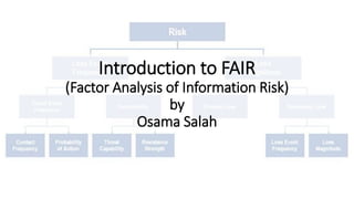
24. The FAIR Risk Ontology
Risk
Loss Event
Frequency
Loss Magnitude
Threat Event
Frequency
Vulnerability
Contact
Frequency
Probability of
Action
Difficulty
Threat
Capability
Primary Loss
Magnitude
Secondary Risk
Secondary
Loss
Magnitude
Secondary
Loss Event
Frequency

25. Risk
The probable frequency and probable magnitude of future loss.
• Probability Based (due to imperfect data and models)
• Informing decision makers on the future potential for loss.
Risk
Loss Event
Frequency
Loss Magnitude

26. Loss Event Frequency (LEF)
The probable frequency, within a given time-frame, that loss will materialize from
a threat-agent’s action.
A measure of how often loss is likely to happen.
There must be a time-frame reference. Given no-time framing, almost any event is
possible.
Typically expressed as a distribution using annualized values.
For example: Between 5 to 25 times per year, with the most likely frequency of 10
times per year.
Expressed as probability if it happens only once.
Risk
Loss Event
Frequency
Loss Magnitude
Min Most Likely Max
5 10 25

27. Threat Event Frequency (TEF)
Risk
Loss Event
Frequency
Loss Magnitude
Threat Event
Frequency
Vulnerability

28. Threat Event Frequency (TEF)
The probable frequency, within a given time-frame, that threat
agents will act in a manner that may result in loss.
Loss Event Frequency (LEF): The probable frequency, within a given time-frame,
that loss will materialize from a threat-agent’s action.
Loss may or may not result from TEF.
Threat Event Loss Event
Hacker attacking website. Hacker damages site or steals information
Pushing new software release to production. Release cause problem leading to downtime, data
integrity issues etc.
Some thrusting a knife at you Getting cut by the knife
Risk
Loss Event
Frequency
Loss Magnitude
Threat Event
Frequency
Vulnerability

29. Threat Event Frequency (TEF)
• Typically expressed as a distribution using annualized values.
• Example: Between 0.1 and 0.5 times per year, with a most likely
frequency of 0.3 time per year. (i.e. between once every 10 years and
once every other year, but most likely every 3 years)
• Expressed as probability if it happens only once.
Risk
Loss Event
Frequency
Loss Magnitude
Threat Event
Frequency
Vulnerability
Min Most Likely Max
0.1 0.3 0.5

30. Contact Frequency
Risk
Loss Event
Frequency
Loss Magnitude
Threat Event
Frequency
Vulnerability
Contact
Frequency
Probability of
Action

31. Contact Frequency (CF)
The probable frequency, within a given time-frame, that threat agents will
come into contact with assets.
Contact Modes: Physical or Logical
Contact Types:
• Random (tornado strike, flu…)
• Regular (cleaning crew comes regularly at 5:15 PM…)
• Intentional (burglar targets specific house)
Typically expressed as annualized distribution. As probability if it happens
only once.
Risk
Loss Event
Frequency
Loss Magnitude
Threat Event
Frequency
Vulnerability
Contact
Frequency
Probability of
Action

32. Probability of Action (PoA)
Risk
Loss Event
Frequency
Loss Magnitude
Threat Event
Frequency
Vulnerability
Contact
Frequency
Probability of
Action

33. Probability of Action (PoA)
The probability that a threat agent will act upon an asset once
contact has occurred.
PoA applies only to threat agents that can think, reason or otherwise
make a decision (humans, animals..) but not acts of nature etc.
(tornados).
The choice to act is driven by:
• Perceived value of the act from the threat agent’s perspective.
• Perceived Level of effort and/or cost from the threat agent’s
perspective.
• Perceived Level of risk to the threat agent.
Risk
Loss Event
Frequency
Loss Magnitude
Threat Event
Frequency
Vulnerability
Contact
Frequency
Probability of
Action

34. Vulnerability
Risk
Loss Event
Frequency
Loss Magnitude
Threat Event
Frequency
Vulnerability
Contact
Frequency
Probability of
Action
Difficulty
Threat
Capability

35. Vulnerability
The probability that a threat agent’s actions will result in loss.
Expressed as a percentage.
The house is 100% vulnerable to damage from a tornado.
The lock is 100% vulnerable to compromise through lock-picking.
That password is 1% vulnerable to brute force attempts.
Usually expressed as a distribution:
That lock is between 5% to 20% vulnerable to lock-picking with a most likely
value of 10%. (i.e. between 5% to 20% of lock picking attempts (most likely
10%)will be successful.
Risk
Loss Event
Frequency
Loss Magnitude
Threat Event
Frequency
Vulnerability
Contact
Frequency
Probability of
Action
Difficulty
Threat
Capability

36. Vulnerability
• Vulnerability exists when there is a difference
between the Threat Capability and the difficulty
to resist.
• Vulnerability is evaluated in the context of the
specific threat types and control types. For
example the difficulty of overcoming anti-virus
controls is irrelevant if the risk analysis is about
insider fraud.
Vulnerability
Difficulty
Threat
Capability

37. Threat Capability (TCap)
Risk
Loss Event
Frequency
Loss Magnitude
Threat Event
Frequency
Vulnerability
Contact
Frequency
Probability of
Action
Difficulty
Threat
Capability

38. Threat Capability (TCap)
The capability of a threat agent.
TCap is a matter of skills (knowledge and experience) and resources
(time & material). With natural threat agents it’s a matter of force.
TCap continuum is a percentiles scale from 1 to 100, which represent
that comprehensive range of capabilities for a population of threat
agents.
Example: Least capable cyber criminal is at the 60th percentile, the
most capable at the 100th and most are at approx. the 90the percentile.
We tend to focus on worst case, but that is thinking in terms of
possibility not probability.
Risk
Loss Event
Frequency
Loss Magnitude
Threat Event
Frequency
Vulnerability
Contact
Frequency
Probability of
Action
Difficulty
Threat
Capability

39. Difficulty (Resistance Strength)
Risk
Loss Event
Frequency
Loss Magnitude
Threat Event
Frequency
Vulnerability
Contact
Frequency
Probability of
Action
Difficulty
Threat
Capability

40. Difficulty
The level of difficulty that a threat agent must overcome.
Difficulty is measured against TCap continuum.
Example:
An authentication control is expected to stop anyone below the 70th
percentile along the TCap continuum. Anyone above the 90th percentile
is certain to succeed. Most likely it’s effective only up to the 85th
percentile.
Risk
Loss Event
Frequency
Loss Magnitude
Threat Event
Frequency
Vulnerability
Contact
Frequency
Probability of
Action
Difficulty
Threat
Capability

41. Difficulty (Resistance Strength)
Relevant controls make the threat agent’s job more difficult (malicious
or act-of-nature scenarios) and easier (in human error scenarios)
Examples from different scenarios
Risk
Loss Event
Frequency
Loss Magnitude
Threat Event
Frequency
Vulnerability
Contact
Frequency
Probability of
Action
Difficulty
Threat
Capability
Malicious Human error Acts of nature
Authentication Training Reinforced construction material
Access privileges Documentation
Patching and Configuration Process simplification
Encryption

42. Loss Magnitude
The probable magnitude of primary and secondary loss resulting from
an event.
Simply: how much tangible loss is expected to materialize from an
event.
Distinguishing between primary and secondary loss is based on
stakeholders and perspective.
Risk
Loss Event
Frequency
Loss Magnitude

43. Loss Magnitude
Primary stakeholders are those individuals or organizations whose
perspective is the focus of the risk. Usually the owner of the primary
asset.
Secondary stakeholder is anyone who is not a primary stakeholder that
may be affected by the loss event being analyzed, and then may react
in a manner that harms the primary stakeholder.
Example: Company X (primary stakeholder) has an event that damages
public health. Direct losses incurred like cleanup are primary losses.
The public (secondary stakeholder) reacts negatively through legal
action, protests, taking business else where etc. these are secondary
losses.
Risk
Loss Event
Frequency
Loss Magnitude

44. Loss Magnitude
Losses on the secondary stakeholder are not put into the formula (not
directly). We would if these losses flow through to the primary
stakeholder.
For example company X might have to compensate member of the
community. These would be included in the secondary loss component.
We can always do a separate risk analysis from the public’s perspective
if that were useful.

45. Primary Loss Magnitude
Primary stakeholder loss that materializes directly as a result of the
event.
Examples:
Lost revenue from operational outages
Wages paid to workers when no work is being performed due to an outage
Replacement of the organization’s tangible assets
Person-hours restoring functionality to assets or operations following an event
Controls Examples:
Disaster Recovery, Business Continuity processes and technologies
Incident response processes
Process or technology redundancies

46. Forms of Loss
Productivity a. Losses resulting from org. ability to execute on its primary value proposition. (revenue lost
when retail website goes down)
b. Losses resulting from personnel being paid but unable to perform their duties. (Failure in
call center)
Consider if revenue is really lost or simply delayed. Can the revenue be recovered? Are all
activities of the personnel effected by they failure?
Response Costs associated with managing the loss event. For example incident response team costs.
Secondary Response costs (expenses incurred dealing with secondary stakeholder) like
notification and credit monitoring costs (confidential records breach)
Replacement The intrinsic value of the asset. The cost to replace the physical asset.
Secondary replacement costs: Refund stolen funds. Replacing credit cards after a credit card
information breach.

47. Forms of Losses
Competitive
Advantage
Losses focused on some asset (physical or logical) that provide an advantage over the
competition. Something another company cannot acquire or develop (legally) on their
own (like intellectual property, secret business plans, market information, patent,
copyrights, trade secrets).
Fines and Judgments
Reputation Effects of reputation loss: market share, cost of capital, stock price, increased cost
hiring/retaining employees.
Reputation losses occur because of a secondary stakeholder perception that and
organization’s value has decreased or liability has increase that affects stakeholders.

48. Secondary Risk
Primary stakeholder loss-exposure that exists due to the potential for
secondary stakeholder reactions to primary event.
Think of it as the fallout from the primary event.
It is driven by:
Secondary Loss Event Frequency (SLEF)
The percentage of primary events that have secondary effects.
Secondary Loss Magnitude
Loss associated with secondary stakeholder reactions.
Risk
Loss Event
Frequency
Loss Magnitude
Primary Loss
Magnitude
Secondary Risk
Secondary
Loss
Magnitude
Secondary
Loss Event
Frequency

49. Secondary Risk
Secondary Loss Event Frequency (SLEF)
The percentage of primary events that have secondary effects.
Company X has environmental loss event of 10 times per year.
Secondary losses materialize only 20% of the time i.e. SLEF is 2 times
per year.
Secondary Loss Magnitude
Examples: Civil, criminal or contractual fined and judgments,
notification costs, public relation costs, legal defense costs, effects of
regulatory sanctions, lost market share, diminished stock price….

50. Are these risks?
Risks?
Cloud Computing Technology
Insider Threat Threat agent
Network share containing sensitive information Assets
Mobile malware Attack vector
Social engineering/phishing Form of attack, technique
Organized crime Threat agent
State sponsored attacks Form of attack
Hacktivists Threat agent
Ransomware Attack vector
Internet of Things Technology
Insecure Passwords Deficient Control

51. FAIR Analysis Process Flow
Scenarios
FAIR
Factors
Expert
Estimation
PERT
Monte
Carlo
Engine
Risk

52. The Tool – End Results
2016
RiskLens
Best Cyber
Risk/Security Tool

53. Source: Measuring and Managing Information Risk – A FAIR Approach

54. Source: Measuring and Managing Information Risk – A FAIR Approach

55. Ransomware Case Study
Source: http://www.risklens.com

56. Ransomware Case study – Options Evaluation
Source: http://www.risklens.com

57. Case Study: Does Training Help Reduce Spear
phishing Risk?
• Training did not show any material reduction of risk associated with phishing campaigns
• Management decided to pursue an alternative phishing-related control, email sandboxing, over training
• Sandboxing has higher costs, but the risk reduction was far more significant (separate analysis conducted)
Source: http://www.risklens.com

58. Case Study: Best architecture to secure cloud
app
Scenario: Understand how much risk is associated with different security encryption strategies related to cloud
data.
Source: http://www.risklens.com

59. Evaluating Different Options