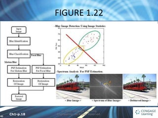
Introduction to Digital Image Processing with MATLAB Asia Edition.ppt

1
© 2010 Cengage Learning
Engineering. All Rights Reserved.
1
Introduction to Digital Image Processing with MATLAB®
Asia Edition
McAndrew‧Wang‧Tseng
Chapter 1:
Introduction

2
1.1 Images and Pictures
• Human have evolved very precise visual skills:
We can identify a face in an instant
We can differentiate colors
We can process a large amount of visual
information very quickly
Ch1-p.1

3
• Image processing involves changing the nature
of an image in order to either
1. improve its pictorial information for human
interpretation, or
2. render it more suitable for autonomous
machine perception
1.2 What Is Image Processing?
Ch1-p.1

4
• Enhancing the edges of an image to make it
appear sharper (Figure 1.1)
• Note how the second image appears cleaner; it is
a more pleasant image
• Sharpening edges is a vital component of printing
Condition 1.
Ch1-p.2

5
FIGURE 1.1
Ch1-p.2

6
• removing noise from an image, noise being
random errors in the image (Figure 1.2)
• removing motion blur from an image. An
example is given in Figure 1.3
• In Figure 1.3(b), it is easier to read the number
plate and to see the spikes on the fence behind
the car, as well as other details not at all clear in
the original image Figure 1.3(a).
Ch1-p.2-3

7
FIGURE 1.2
Ch1-p.3

8
FIGURE 1.3
Ch1-p.3

9
• Obtaining the edges of an image (Figure 1.4)
• Once we have the edges we can measure their
spread and the area contained within them
• We can also use edge-detection algorithms as a
first step in edge enhancement
Condition 2.
Ch1-p.3-4

10
FIGURE 1.4
Ch1-p.4

11
• For measurement or counting purposes, we may
not be interested in all the detail in an image
(Figure 1.5)
• We could, for example, measure the size and
shape of the animal without being distracted by
unnecessary detail
Ch1-p.4-5

12
FIGURE 1.5
Ch1-p.4

13
1.3 Image Sampling and Acquisition
• Sampling refers to the process of digitizing a
continuous function
• e.g.,
 sample it at 10 evenly spaced values of x only
(Figure 1.6)
 sample it at 100 points, as shown in Figure 1.7
Ch1-p.5

14
FIGURE 1.6
Ch1-p.5

15
FIGURE 1.7
Ch1-p.5

16
1.3 Image Sampling and Acquisition
• Nyquist criterion which says, in effect, that a
continuous function can be reconstructed from
its samples provided that the sampling frequency
is at least twice the maxi-mum frequency in the
function
Ch1-p.5

17
FIGURE 1.8
Ch1-p.6

18
• Image Acquisition
 CCD CAMERA
FIGURE 1.9
Ch1-p.7

19
FIGURE 1.10
 FLAT-BED SCANNER
Ch1-p.8

20
FIGURE 1.11
 OTHER ENERGY SOURCES
Ch1-p.8

21
FIGURE 1.12
Ch1-p.9

22
1.4 Images and Digital Images
• We may consider this image as being a two-
dimensional function f (x, y)
• We may assume that in such an image, brightness
values can be any real numbers in the range 0.0 (black)
to 1.0 (white)
• The f (x, y) values in a digital image take only integer
values ranging from 1 to 256 each and the brightness
values ranging from 0 (black) to 255 (white)
Ch1-p.9-10

23
FIGURE 1.13
Ch1-p.10

24
FIGURE 1.14
Ch1-p.11

25
1.4 Images and Digital Images
• A digital image can be considered as a large array
of sampled points from the continuous image
• These points are the pixels, which constitute the
digital image
• The pixels surrounding a given pixel constitute its
neighborhood.
Ch1-p.10

26
FIGURE 1.15
Ch1-p.11

27
1.5 Some Applications
• Medicine
• Agriculture
• Industry
• Law enforcement
Ch1-p.11-12

28
1.6 Aspects of Image Processing
• IMAGE ENHANCEMENT
 sharpening or deblurring an out-of-focus image
 highlighting edges,
 improving image contrast or brightening an image, and
 removing noise
• IMAGE RESTORATION
 removing of blur caused by linear motion,
 removal of optical distortions, and
 removing periodic interference
Ch1-p.12

29
1.6 Aspects of Image Processing
• IMAGE SEGMENTATION
 finding lines, circles, or particular shapes in an image, and
 identifying cars, trees, buildings, or roads in an aerial
photograph
• A given algorithm may be used for both image
enhancement or for image restoration
Ch1-p.12-13

30
1.7 An Image-Processing Task
• Acquiring the image
• Preprocessing
• Segmentation
• Representation and description
• Recognition and interpretation
Ch1-p.13

31
FIGURE 1.16
• Binary
Ch1-p.14

32
FIGURE 1.17
• Grayscale
Ch1-p.14

33
FIGURE 1.18
• True color or red-green-blue
Ch1-p.15

34
FIGURE 1.19
• Indexed
Ch1-p.16

35
1.9 Image File Sizes
• A 512 × 512 binary image
• A grayscale image
(Divided by 8)
Ch1-p.16

36
1.9 Image File Sizes
• A Color image
Ch1-p.17

37
1.10 Image Perception
• We should be aware of the limitations of the
human visual system
 Observed intensities vary as to the background
 We may observe nonexistent intensities as bars in
continuously varying gray levels
 Our visual system tends to undershoot or overshoot
around the boundary of regions of different
intensities
Ch1-p.17-18

38
FIGURE 1.20
Ch1-p.17

39
FIGURE 1.21
Ch1-p.18

40
FIGURE 1.22
Ch1-p.18

Introduction to Digital Image Processing with MATLAB Asia Edition.ppt

More Related Content

Similar to Introduction to Digital Image Processing with MATLAB Asia Edition.ppt

Recently uploaded

Introduction to Digital Image Processing with MATLAB Asia Edition.ppt