IJEBEA14-419

International Association of Scientific Innovation and Research (IASIR)
(An Association Unifying the Sciences, Engineering, and Applied Research)
International Journal of Engineering, Business and Enterprise
Applications (IJEBEA)
www.iasir.net
ISSN (Print): 2279-0020
ISSN (Online): 2279-0039
Performance Evaluation for Productivity Management
1
Ajin T Thomas, 2
Anup Nair
1
M.Tech. Scholar, Industrial Engg. & Management
2
Assistant Professor, Dept. of Mechanical Engg.
1, 2
Mangalam College of Engineering,
Kottayam, Kerala, INDIA
__________________________________________________________________________________________
Abstract: Productivity management is one of the major problems faced by many firms all over the world.
Without identifying productivity influence factor it is difficult to manage the production cycle. The paper
concentrates on the evaluation of management controls over the production. The day to day productivity must
be measure and compare for to take corrective actions and to increase the productivity. This paper presents a
project work done in a small scale footwear industry in south India. Few research efforts have specifically
evaluated productivity in the context of the productivity management cycle. Consequently, there is still a lack of
useful indicators for determining which items should be prioritized and improved upon in order to yield the
highest benefits from productivity management. In an effort to address this issue, this study proposes a method
for calculating productivity. Tool used for the project is Productivity Achievement Ratio (PAR), Regression
analysis, Relative Importance Index (RII) etc.
Keywords: PAR, OP, AP, RII, Variable Ranking, Reduction Factors etc.
_______________________________________________________________________________________
I. INTRODUCTION
Productivity-one of the major factors used in measuring industry outcomes- is defined as the relation between a
production system output and the input set in that system. The importance of managing productivity has long
been emphasized in the manufacturing industry, and a considerable amount of research has been conducted on
the issue. Both managers and employees should pay close attention to productivity management and that the
productivity management cycle has four phases: measurement, evaluation, planning, and improvement. There
have been many research efforts to examine productivity measurement and consequently contribute to the better
productivity management However, despite yielding decent estimations of productivity, these studies have
rarely identified which items require the most attention for optimal productivity management. Indeed,
productivity has commonly been estimated by the ratio between system output and input without consideration
of the particulars of each work item. Considering each work item when measuring productivity is a complex
process. For instance, it must be taken into account that work items associated with low productivity do not
always have high potential for improvement. As well, a minimal change in productivity does not necessarily
signify the presence of a work item linked with a poor management performance. To deal with these
complexities, an advanced productivity indicator, which can account for the unique characteristics of each item,
is needed. This work is done for the enhancement of productivity and reduces the productivity fluctuations in a
small scale footwear industry in Kerala, India (Footmate polymer Footwears India Pvt. Ltd- a LUNAR Group of
company).
For example, Table 1 shows the labor productivity calculated using the data collected from FOOTMATE for the
months of April and March in packing unit. As seen in Table 1, the productivity of the month March is 103.02,
while that of the month April is 132.96. However, this fact does not directly indicate that the productivity
management of the month April is better than that of the month March. It would also be inappropriate to
conclude that the month April has higher potential for improvement than the month March. Instead, it must be
determined which of the Month should be focused on during the planning and improvement phases of the
productivity management cycle. These items should not be chosen merely by estimating productivity without
considering the potential effects of management activity. Although conversion factors can be used to account for
different labor resources and conditions required for the outputs, they still do not provide clear information
regarding the potential effects of management activity. Thus, this research aims at developing a productivity
evaluation indicator that takes management aspects into account so that the most appropriate items for
management activity are selected, and so that the benefits of productivity are maximized.
Table 1: Labor Productivity of PACKING UNIT in FOOTMATE.
WORKERS(A) TOTAL UNITS(B) PRODUCTIVITY (B/A)
MARCH 227 23385 103.02
APRIL 239 31778 132.96

Ajin T Thomas et al., International Journal of Engineering, Business and Enterprise Applications, 10(1), September-November, 2014, pp.
41-51
IJEBEA 14-419; © 2014, IJEBEA All Rights Reserved Page 42
II. LITERATURE REVIEW
A. Productivity
Prokopenko defined that “productivity is the relationship between the output generated by a production or
service system and the input provided to create this output. Thus, productivity is defined as the efficient use of
resource – labors, capital, land, materials, energy and information – in the production of various goods or
services. Productivity can also be defined as the relationship between results and the time it takes to accomplish
them. Time is often a good denominator since it is a universal measurement and it beyond human control. The
less time taken to achieve the desired result is the more productive the system”. Prokopenko also stated that
“regardless the type of production, economic or political system, the definition of productivity remains the
same. Thus, though productivity may mean different things to different people, the basic concept is always the
relationship between the quantity and quality of goods or services produced and the quantity of resources used
to produce them”.
Eatwell and Newman (1991) defined productivity as a ratio of some measure of output to some index of input
use. Put differently, productivity is nothing more than arithmetic ratio between the amount produced and the
amount of any resources used in the course of production. This conception of productivity goes to imply that it
can indeed be perceived as the output per unit input. Overall, productivity could be defined as the ratio of
outputs to inputs
Productivity = Outputs / Inputs
B. Productivity improvement methods
There is several productivity improvement methods developed so far. Shruti Sehgal categorized the methods
into seven basic categories namely, employee based, material based, task based, management based, technology
based, product based and investment based. And any other techniques can be grouped in any of these categories
[8]. Anton Soekiman summarized manufacturing system productivity improvement methods into operation
research based, system analysis based, continuous improvement based and performance metrics based. [10]
Shruti Sehgal represented the productivity improvement methods into the following categories: logistics,
quality, production engineering and others [8]
C. Actual Productivity and Obtainable Productivity
Tae Wan Kim et al [1] assumes that there exists productivity yielded under an ideal situation. Such productivity
is defined as Ideal Productivity (IP). In contrast, Actual Productivity (AP) is yielded in reality where various
factors can prevent the attainment of IP. In addition to IP and AP, there exists Obtainable Productivity (OP). OP
is the maximum productivity that can be attained through the adequate management of controllable variables.
D. Reduction Factors
A Reduction Factor (RF) is defined by Tae Wan Kim et al [1] as a factor that prevents productivity from
reaching an IP value. Namely, an RF makes the difference between IP and AP. This idea is formalized in the
following equation:
AP = IP – an amount of productivity loss caused by RF
Only a factor can be an RF, not an event. For example, although “overtime” causes productivity to decrease, it
cannot be called an RF because it is an event. In this case, “insufficient time” is considered a factor and
therefore an RF.
E. Factors affecting productivity
Mr. A .A. Attar et al [2] states that the Factors affecting labor productivity have been identified and are grouped
into 15 categories according to their characteristics, namely 1)Design factors 2) Execution plan factors 3)
Material factors 4) Equipment factors 5) Labor factors 6) Health and safety factors 7) Supervision factors 8)
Working time factors 9) Project factors 10) Quality factors 11) Financial factors 12) Leadership and
coordination factors 13) Organization factors 14) Owner/consultant factors 15) External factors
The top ten factors that affect the small and medium company: 1) Lack of material 2) Labor strikes 3) Delay in
arrival of materials 4) Financial difficulties of the owner 5) Unclear instruction to laborer and high absenteeism
of labors 6) Bad weather (e.g. rain, heat, etc.) 7) Non discipline labor and use of alcohol and drugs 8) No
supervision method, design changes, repairs and repetition of work, and bad resources management 9) Bad
supervisors absenteeism and far away from location of material storage, and 10) Bad leadership
There are various literatures that illustrate the relation between some of these factors and the productivity of the
employee. There are different reduction factors identified by the authors of various literature and these reduction
factors and variables were reviewed.
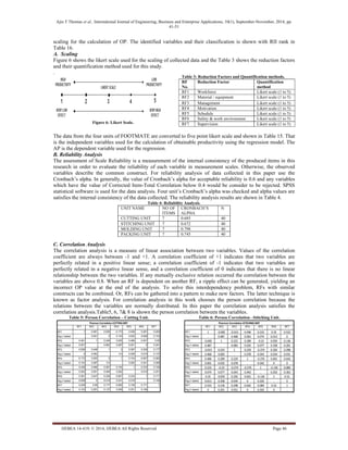
F. Productivity Achievement Ratio (PAR)
The Productivity Achievement Ratio (PAR) can be represented as the quotient of AP and OP. This value
considers the potential effect of improvement and therefore can be used as a productivity evaluation indicator to
determine the main items that should be focused on during production. The PAR formulated by Tae Wan Kim et
al [1]. But these methods have lot of difficulties within that that was focused to review and suggest new method

41-51
and practically justify using the new method. The classification and the statistical method used in that paper was
statistically irrelevant for the use.
G. Relative Importance Index (RII)
The aim of the analysis was to establish the relative importance of the various factors identified as responsible
for production variation. The score for each factor is calculated by counting the scores from the observations.
The relative importance index (RII) was calculated using the following formula.
5 4 3 2 15 * 4 * 3 * 2 * 1*
(% ) *100
5 *
n n n n n
RII
N
   
 (1)
Where,
n1 - n5 is the no of observation results 1 to 5
N is the total no of observation.
III. DEFINITIONS
A. Productivity
This research assumes that there exists productivity yielded under an ideal situation. Such productivity is
defined as Ideal Productivity (IP). In contrast, Actual Productivity (AP) is yielded in reality where various
factors can prevent the attainment of IP. In addition to IP and AP, there exists Obtainable Productivity (OP). OP
is the maximum productivity that can be attained through the adequate management of controllable variables.
The differences between OP and baseline productivity (BP) are determined, as shown in Table 2.
Table 2: Comparison of Baseline Productivity and Obtainable Productivity.
Baseline productivity Obtainable productivity
The maximal productivity (or top
10%) obtained within the project
Productivity obtained from the most controllable situation.
1:1 function to event Focusing on factors, not events
Pre-set from existing data and therefore unchangeable
over time.
Calculated by current site data. As time passes and data is accumulated,
accuracy increases.
Figure 1: Comparing Baseline Productivity with Obtainable
Productivity.
Figure 2: Relationship of Reduction Factors and
Productivity.
Figure 1 illustrates those differences. Dots in the Figure represent the daily results of productivity (AP). The Y
axis is productivity as a unit-rate. That is, if less amount of input is required for one unit-work, a higher
productivity is yielded. The daily amount of productivity is constantly changing. Regardless of changes in
project circumstance, baseline productivity is set by the median of the daily productivity values in the baseline
subset which is 10% of the total workdays. However, OP is changing on a daily basis according to changes in
project circumstances. It is notable that OP does not necessarily follow the same pattern as the actual
productivity curve.
B. Reduction Factors
A Reduction Factor (RF) is defined as a factor that prevents productivity from reaching an IP value. Namely, an
RF makes the difference between IP and AP. This idea is formalized in the following equation:
AP = IP – an amount of productivity loss caused by RF (2)
Can the RF be controlled by Anyone Working on the Site?
Managers can control factors, such as “site layout plans,” that can potentially obstruct AP from reaching OP.
However, other factors, such as “weather conditions,” cannot be controlled or stopped, therefore preventing OP
from reaching IP. While the former factor type is referred to as a Controllable-RF (C_RF), the latter is referred
to as an Uncontrollable-RF (UC_RF). These concepts are presented in the following equations:

41-51
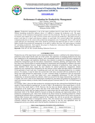
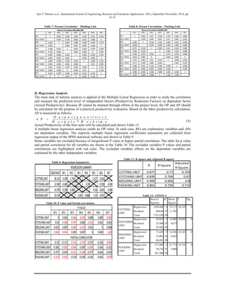
OP = IP – an amount of productivity loss caused by UC_RF (3)
AP = OP – an amount of productivity loss caused by C_RF (4)
Figure 2 visualizes the relationship between RFs and productivity
While some RFs, such as “worker faithfulness,” change from day to day, other RFs, such as “Plant Lay out,”
remain unchanged over the course of production. The former RF type is called a Variable-RF (V_RF), while the
latter is called an Invariable-RF (IV_RF). Previous researcher says that the Invariable reduction factors do not
have an impact on the productivity. But, Invariable reduction factors have serious impact on the productivity
and the invariable reduction factors effects are vary over time. KIM Tae Wan [1] classifies the variables into
Invariable and Variable Reduction factors and excludes the invariable RF. In this study not classifies the
reduction factors into the variable or invariable. In this study classify the variables into Controllable and
Uncontrollable and then grouped the variables according to their characteristics. The Uncontrollable variables
are classified separately.
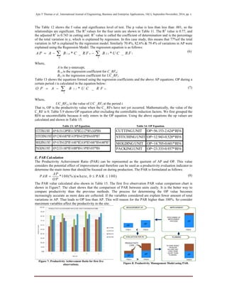
IV. METHODOLOGY
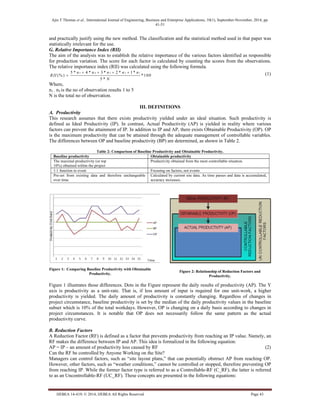
A. Research Process
The research process consists of 7 steps illustrate in Figure 3. In step 1 define the research problem and conduct
a detailed literature review. In next step determine a data collection method and develop a plan for data analysis.
Through Literature review and pilot survey identify the variables affect productivity and short list it. In step 3
conducts a pilot survey to short list the variables affect the productivity and classify according to the
characteristics of the variables. Next stage is to design the observation data sheet and collect the data through
field observation. The scaling of the data is done with this step. In data analysis stage Conduct reliability
analysis to find the data is significant or not. And a correlation analysis need to conduct because to identify any
mutually exclusive relation between the variables. Through forming a regression equation calculates the value
of obtainable productivity and then calculates the productivity achievement ratio. As part of that rank the
variables with relative importance index, it help to prioritized problem solving.
Figure 3: Research Process.
Figure 4: Variable ranking Procedure

Ajin T Thomas et al., International Journal of Engineering, Business and Enterprise Applications, 10(1), September-November, 2014, pp. x
Figure 5: Comparison of Productivity between Item A and Item B
B. Sampling Design
In FOOTMATE Polymer Footwear’s India Pvt. Ltd have four production units in their poly urethane footwear
manufacturing factory namely cutting unit, stitching unit, molding unit & packing units. All these units are
comes under the study. In this project choose total population sampling, necessary to study the entire
population of FOOTMATE Polymer Footwear’s India Pvt. Ltd because the size of the population that has the
particular set of characteristics that we are interest in is typically very small.
C. Pilot Survey
There are two phases in research design step of this study are pilot survey and main survey. Pilot survey used
collect the factors that observe in the field reduce productivity and site conditions. Pilot survey also helps to
interact with the company officials to identify the variations in productivity. Main survey consists of the field
observation. Based on the literature review identify the variables affecting productivity. Some variables are
listed by the basis on the conversation with the employees. On the basis of the listed variables a pilot survey is
conducted for short list the variables by the frequency of observation.
The variables short listed by observe the field and on the basis of opinion of the officials and employees. In
summary, based on the previous research, pilot survey, refinement and discussion with experts, 46 Variables are
selected and these are grouped to 7 Factors according to their characteristics, namely: Workforce,
material/equipment, management, motivation, schedule, Safety and Work environment and supervision. Out of
this Safety and Work environment is a group of uncontrollable variable and other factors are the group of
controllable variables.
The observation data sheet designed for a natural field survey and the data sheet consist of the 38 controllable
and 8 uncontrollable variables identified. The time scheduled to make this observation is from 8.00 am to 6.30
pm of every working day of the company. Company has only one shift and work time of employees except the
stitching unit is 8.4 hour and duty time of stitching unit was 9.1 hour. RFs and productivity data are collected
periodically.
D. Data Collection
The data collection method used in this survey is field observation. The reason why this method chosen because
is FOOTMATE is a small scale industry and consist of uneducated workers only. So the questionnaire survey
and interview method is not possible in this survey. Herbsman and Ellis (1990) have recommended that the
minimum number of observations should be at least three times the number of the RFs involved in a specific
item. For example, if there are 10 RFs, then 30 or more cases should be collected.
E. Data Analysis
In data analysis scales the collected data and conduct a reliability analysis, Correlation analysis. Next step is to
calculate the productivity achievement ratio. Figure 4 shows the overall procedure for calculation of
Productivity Achievement Ratio and Variable Ranking. An item with a high PAR indicates that the item’s
productivity has been managed effectively. On the contrary, an item with a low PAR should be carefully
monitored and studied to improve on-site productivity. For example, in Figure 5, though the AP of item A is
higher than that of item B, item A should be prioritized by site management because the PAR (
PAR=AP*100/OP) of item A is 50%, while the PAR of item B is 67%. Managers should investigate the main
culprit of the productivity loss and make efforts to reduce or minimize the cause. Since it is non-dimensional,
the PAR can be used to compare the same items among different units with different C_RFs.
V. DATA ANALYSIS AND INTERPRETATION
The variables frequency of occurrence will be measured for forty days. The frequencies of occurrence of
variables are used for the calculation of Relative Importance Index. The total of each variable group are used for

41-51
scaling for the calculation of OP. The identified variables and their classification is shown with RII rank in
Table 16.
A. Scaling
Figure 6 shows the likert scale used for the scaling of collected data and the Table 3 shows the reduction factors
and their quantification method used for this study.
.
Figure 6: Likert Scale.
Table 3: Reduction Factors and Quantification methods.
RF
No.
Reduction Factor Quantification
method
RF1 Workforce Likert scale (1 to 5)
RF2 Material / equipment Likert scale (1 to 5)
RF3 Management Likert scale (1 to 5)
RF4 Motivation Likert scale (1 to 5)
RF5 Schedule Likert scale (1 to 5)
RF6 Safety & work environment Likert scale (1 to 5)
RF7 Supervision Likert scale (1 to 5)
The data from the four units of FOOTMATE are converted to five point likert scale and shown in Table 15. That
is the independent variables used for the calculation of obtainable productivity using the regression model. The
AP is the dependent variable used for the regression.
B. Reliability Analysis
The assessment of Scale Reliability is a measurement of the internal consistency of the produced items in this
research in order to evaluate the reliability of each variable in measurement scales. Otherwise, the observed
variables describe the common construct. For reliability analysis of data collected in this paper use the
Cronbach’s alpha. In generally, the value of Cronbach’s alpha for acceptable reliability is 0.6 and any variables
which have the value of Corrected Item-Total Correlation below 0.4 would be consider to be rejected. SPSS
statistical software is used for the data analysis. Four unit’s Cronbach’s alpha was checked and alpha values are
satisfies the internal consistency of the data collected. The reliability analysis results are shown in Table 4.
Table 4: Reliability Analysis.
UNIT NAME NO OF
ITEMS
CRONBACH’S
ALPHA
N
CUTTING UNIT 7 0.685 40
STITCHING UNIT 7 0.672 40
MOLDING UNIT 7 0.798 40
PACKING UNIT 7 0.745 40
C. Correlation Analysis
The correlation analysis is a measure of linear association between two variables. Values of the correlation
coefficient are always between -1 and +1. A correlation coefficient of +1 indicates that two variables are
perfectly related in a positive linear sense; a correlation coefficient of -1 indicates that two variables are
perfectly related in a negative linear sense, and a correlation coefficient of 0 indicates that there is no linear
relationship between the two variables. If any mutually exclusive relation occurred the correlation between the
variables are above 0.8. When an RF is dependent on another RF, a ripple effect can be generated, yielding an
incorrect OP value at the end of the analysis. To solve this interdependency problem, RFs with similar
constructs can be combined. Or, RFs can be gathered into a pattern to make new factors. The latter technique is
known as factor analysis. For correlation analysis in this work chooses the person correlation because the
relations between the variables are normally distributed. In this paper the correlation analysis satisfies the
correlation analysis.Table5, 6, 7& 8 is shown the person correlation between the variables.
Table 5: Person Correlation – Cutting Unit. Table 6: Person Correlation –Stitching Unit.
RF1 RF2 RF3 RF4 RF5 RF6 RF7
RF1 1 0.461 0.526 -0.173 0.436 0.381 0.205
Sig.(1-tailed . 0.001 0 0.143 0.002 0.008 0.103
RF2 0.461 1 0.248 0.005 0.486 0.547 0.09
Sig.(1-tailed 0.001 . 0.062 0.487 0.001 0 0.291
RF3 0.526 0.248 1 0 0.397 0.329 0.177
Sig.(1-tailed 0 0.062 . 0.5 0.006 0.019 0.137
RF4 -0.173 0.005 0 1 0.104 -0.067 -0.082
Sig.(1-tailed 0.143 0.487 0.5 . 0.262 0.341 0.308
RF5 0.436 0.486 0.397 0.104 1 0.333 0.109
Sig.(1-tailed 0.002 0.001 0.006 0.262 . 0.018 0.251
RF6 0.381 0.547 0.329 -0.067 0.333 1 0.171
Sig.(1-tailed 0.008 0 0.019 0.341 0.018 . 0.146
RF7 0.205 0.09 0.177 -0.082 0.109 0.171 1
Sig.(1-tailed 0.103 0.291 0.137 0.308 0.251 0.146 .
Pearson Correlation-CUTTINGUNIT
RF1 1 ‐0.005 ‐0.013 0.496 0.233 0.35 0.533
Sig.(1-tailed . 0.487 0.468 0.001 0.074 0.013 0
RF2 ‐0.005 1 0.223 0.289 ‐0.23 0.059 0.136
Sig.(1-tailed 0.487 . 0.083 0.035 0.077 0.358 0.201
RF3 ‐0.013 0.223 1 0.229 ‐0.274 0.292 0.298
Sig.(1-tailed 0.468 0.083 . 0.078 0.043 0.034 0.031
RF4 0.496 0.289 0.229 1 ‐0.276 0.601 0.642
Sig.(1-tailed 0.001 0.035 0.078 . 0.042 0 0
RF5 0.233 ‐0.23 ‐0.274 ‐0.276 1 ‐0.136 0.084
Sig.(1-tailed 0.074 0.077 0.043 0.042 . 0.202 0.302
RF6 0.35 0.059 0.292 0.601 ‐0.136 1 0.52
Sig.(1-tailed 0.013 0.358 0.034 0 0.202 . 0
RF7 0.533 0.136 0.298 0.642 0.084 0.52 1
Sig.(1-tailed 0 0.201 0.031 0 0.302 0 .
Pearson Correlation-STICHINGUNIT

41-51
Table 7: Person Correlation – Molding Unit. Table 8: Person Correlation – Packing Unit.
D. Regression Analysis
The main task of statistic analysis is applied in the Multiple Linear Regression in order to study the correlation
and measure the prediction level of independent factors (Productivity Reduction Factors) on dependent factor
(Actual Productivity). Because IP cannot be attained through efforts at the project level, the OP and AP should
be calculated for the purpose of a practical productivity evaluation. Based on the labor productivity calculation,
AP is measured as follows:
(5)
Actual Productivity of the four units will be calculated and shown Table 15.
A multiple linear regression analysis yields an OP value. In each case, RFs are explanatory variables and APs
are dependent variables. The stepwise multiple linear regression coefficients summaries are collected from
regression output of the SPSS statistical software and shown in Table 9.
Some variables are excluded because of insignificant P value or higher partial correlation. The table for p value
and partial correlation for all variables are shown in the Table 10. The excluded variables P values and partial
correlations are highlighted with red color. The excluded variables effects on the dependent variables are
explained by the other independent variables.
Table 11: R square and Adjusted R square
Table 9: Regression Summaries
Table 10: P value and Partial correlation.
Table 12: ANNOVA
RF1 1 0.292 0.166 0.497 0.345 0.221 0.514
Sig.(1-tailed . 0.034 0.154 0.001 0.015 0.085 0
RF2 0.292 1 0.467 0.384 0.308 0.305 0.579
Sig.(1-tailed 0.034 . 0.001 0.007 0.026 0.028 0
RF3 0.166 0.467 1 0.467 0.244 0.579 0.269
Sig.(1-tailed 0.154 0.001 . 0.001 0.065 0 0.047
RF4 0.497 0.384 0.467 1 0.292 0.444 0.514
Sig.(1-tailed 0.001 0.007 0.001 . 0.034 0.002 0
RF5 0.345 0.308 0.244 0.292 1 0.264 0.313
Sig.(1-tailed 0.015 0.026 0.065 0.034 . 0.05 0.025
RF6 0.221 0.305 0.579 0.444 0.264 1 0.191
Sig.(1-tailed 0.085 0.028 0 0.002 0.05 . 0.118
RF7 0.514 0.579 0.269 0.514 0.313 0.191 1
Sig.(1-tailed 0 0 0.047 0 0.025 0.118 .
Pearson Correlation-MOLDINGUNIT
RF1 1 0.282 0.271 0.344 0.197 0.466 0.083
Sig.(1-tailed . 0.039 0.045 0.015 0.111 0.001 0.305
RF2 0.282 1 0.118 0.422 0.063 0.451 0.046
Sig.(1-tailed 0.039 . 0.234 0.003 0.349 0.002 0.389
RF3 0.271 0.118 1 0.563 0.43 0.316 0.382
Sig.(1-tailed 0.045 0.234 . 0 0.003 0.023 0.008
RF4 0.344 0.422 0.563 1 0.274 0.434 0.608
Sig.(1-tailed 0.015 0.003 0 . 0.044 0.003 0
RF5 0.197 0.063 0.43 0.274 1 0.058 0.205
Sig.(1-tailed 0.111 0.349 0.003 0.044 . 0.362 0.103
RF6 0.466 0.451 0.316 0.434 0.058 1 ‐0.042
Sig.(1-tailed 0.001 0.002 0.023 0.003 0.362 . 0.399
RF7 0.083 0.046 0.382 0.608 0.205 ‐0.042 1
Sig.(1-tailed 0.305 0.389 0.008 0 0.103 0.399 .
Pearson Correlation-PACKINGUNIT
CONSTANT RF1 RF2 RF3 RF4 RF5 RF6 RF7
CUTTING UNIT 56.153 ‐3.249 ‐1.742 ‐2.127 ‐2.624
STITCHING UNIT 12.943 ‐0.483 ‐0.39 ‐0.528 ‐0.458
MOLDING UNIT 14.705 ‐0.328 ‐0.481 ‐0.36 ‐0.601 ‐0.468
PACKING UNIT 23.333 ‐1.043 ‐0.888 ‐1.54 ‐0.937
REGRESSION SUMMARY
CUTTING UNIT 0 0.042 0.446 0.105 0.008 0.009 0.585
STITCHING UNIT 0.02 0.589 0.797 0.085 0.233 0.025 0.052
MOLDING UNIT 0.023 0.007 0.069 0.333 0.023 0 0.008
PACKING UNIT 0.063 0.941 0.001 0.007 0 0.004 0.83
CUTTING UNIT ‐0.32 ‐0.171 ‐0.131 0.275 ‐0.227 ‐0.226 0.094
STITCHING UNIT ‐0.381 ‐0.093 ‐0.044 ‐0.287 ‐0.204 ‐0.369 ‐0.322
MOLDING UNIT ‐0.377 ‐0.443 ‐0.311 ‐0.168 ‐0.377 ‐0.664 ‐0.433
PACKING UNIT ‐0.313 0.013 ‐0.519 ‐0.439 ‐0.545 ‐0.465 0.037
P VALUE
PARTIAL CORRELATION
CUTTING UNIT 0.877 0.77 0.743
STITCHING UNIT 0.839 0.704 0.67
MOLDING UNIT 0.909 0.826 0.8
PACKING UNIT 0.891 0.794 0.771
R R Square
Adjusted
R Square
Sumof
Squares
df Mean
Square
F Sig.
Regression 1349.469 4 337.37 29.223 0
Residual 404.06 35 11.545
Total 1753.529 39
Regression 56.025 4 14.006 20.802 0
Residual 23.566 35 0.673
Total 79.592 39
Regression 71.429 5 14.286 32.247 0
Residual 15.062 34 0.443
Total 86.491 39
Regression 271.089 4 67.772 33.753 0
Residual 70.276 35 2.008
Total 341.366 39
CUTTING
UNIT
STITCHING
UNIT
MOLDING
UNIT
PACKING
UNIT
( )
k e r *
O u t p u t q u a n t i t i e s
A P
W o r s W o r k t i m e


The Table 12 shows the f value and significance level of test. The p value is less than less than .001, so the
relationships are significant. The R2
values for the four units are shown in Table 11. The R2
value is 0.77, and
the adjusted R2
is 0.743 in cutting unit. R2
value is called the coefficient of determination and is the percentage
of the total variation in y, which is explained by regression. In this case study, this means that 77%of the total
variation in AP is explained by the regression model. Similarly 70.4%, 82.6% & 79.4% of variations in AP were
explained using the Regression Model. The regression equation is as follows:
(6)
Where,
A is the y-intercept;
B1,n is the regression coefficient for C_RFn;
B2,l is the regression coefficient for UC_RFl.
Table 13 shows the equations formed using the regression coefficients and the above AP equations. OP during a
certain period t is calculated in the equation below:
(7)
Where,
UC_RFl,t is the value of UC _RFl at the period t.
That is, OP is the productivity value when the C_ RFs have not yet occurred. Mathematically, the value of the
C_RF is 0. Table 5.9 shows OP equation after excluding the controllable reduction factors. We first grouped the
RF6 as uncontrollable because it only enters in the OP equation. Using the above equations the op values are
calculated and shown in Table 15.
Table 13: AP Equation. Table 14: OP Equation.
E. PAR Calculation
The Productivity Achievement Ratio (PAR) can be represented as the quotient of AP and OP. This value
considers the potential effect of improvement and therefore can be used as a productivity evaluation indicator to
determine the main items that should be focused on during production. The PAR is formulated as follows:
(8)
The PAR value calculated also shown in Table 15. The first five observation PAR value comparison chart is
shown in Figure7. The chart shows that the comparison of PAR between units easily. It is the better way to
compare productivity than the previous methods. The process for determining the OP value becomes
increasingly accurate as more data are collected. If the variables considered are explain fewer amount of total
variations in AP. That leads to OP less than AP. This will reason for the PAR higher than 100%. So consider
maximum variables affect the productivity in the site.
Figure 7: Productivity Achievement Ratio for first five
observations. Figure 8: Productivity Management Model using PAR.
CUTTINGUNIT AP=56.153-3.249*RF1-1.742*RF2-2.127*RF5-2.624*RF6
STITCHINGUNIT AP=12.943-0.483*RF1-0.39*RF4-0.528*RF6-0.458*RF7
MOLDINGUNIT AP=14.705-0.328*RF1-0.481*RF2-0.36*RF5-0.601*RF6-0.468*RF7
PACKINGUNIT AP=23.333-1.043*RF3-0.888*RF4-1.54*RF5-0.937*RF6
CUTTINGUNIT OP=56.153-2.624*RF6
STITCHINGUNIT OP=12.943-0.528*RF6
MOLDINGUNIT OP=14.705-0.601*RF6
PACKINGUNIT OP=23.333-0.937*RF6
1, 2 ,* _ * _n n l l
n l
A P A B C R F B U C R F   
2 , * _l l t
l
O P A B U C R F  
*100(% )(where, 0 PAR 100)
AP
PAR
OP
  

F. Relative Importance Index (RII)
Relative importance index was used here for the ranking of variables affect the productivity. In this work each
of the 46 variables RII will be calculated and for four units separately using equation 1. The results are shown in
table 16. From the ranking managers can identify which variables are most affected in the factory. RII was
calculated using the frequency of occurrence of variables in the factory.
G. Productivity Management Using the PAR and RII
As a productivity evaluation indicator, the PAR can assist managers in identifying the management items that
require productivity improvement the most. The PAR does this by focusing on an item’s potential for
improvement. In Figure 8, although item B has a better productivity value than item A, more intensive
management is required for item B. Therefore, causes of the productivity loss of item B can be investigated and
short-term and long-term plans can be established to reduce the productivity loss. Then, the process for
improving the actual productivity of item B can be performed to acquire higher PAR. Likewise, the PAR can be
used for a comparison of the same items from different units and for a comparison of different items at the same
units.
Table 15: OP and PAR Calculation.
It must be taken into account that the prioritization of PAR improvement can be affected by factors other than
productivity itself. For example, when it is relatively expensive to improve the PAR of an item, the current
production system might be kept in place for the sake of cost-effectiveness. From an organizational perspective,
RF1RF2 RF3 RF4RF5 RF6 RF7 RF1RF2 RF3 RF4 RF5 RF6 RF7 RF1RF2 RF3 RF4RF5 RF6 RF7 RF1RF2 RF3 RF4 RF5 RF6 RF7
1 28.93 2 3 2 2 3 2 1 50.9 56.8 9.313 2 2 1 2 2 3 2 11.4 81.99 10.23 3 2 1 2 3 1 3 14.1 72.53 16.63 2 1 1 2 2 3 1 20.52 81.02
2 33.93 3 2 3 2 2 2 1 50.9 66.7 9.794 2 1 1 2 2 3 2 11.4 86.22 9.81 1 2 2 3 2 3 2 12.9 76.01 14.81 0 2 3 2 3 2 2 21.46 68.99
3 26.95 2 4 2 2 4 3 2 48.3 55.8 8.338 3 3 2 3 3 3 3 11.4 73.4 8.08 3 3 2 3 4 2 4 13.5 59.84 18.21 2 1 1 1 2 2 0 21.46 84.88
4 26.48 3 3 3 1 3 3 2 48.3 54.8 11.33 1 1 1 0 3 1 1 12.4 91.29 10.00 1 2 1 2 3 2 2 13.5 74.06 19.71 1 1 0 1 2 0 2 23.33 84.49
5 37.08 2 2 2 3 2 2 0 50.9 72.8 8.227 2 3 1 3 1 3 2 11.4 72.43 10.52 3 1 2 2 2 2 2 13.5 77.94 18.64 1 2 1 2 1 2 1 21.46 86.88
6 34.58 3 2 1 1 2 2 2 50.9 67.9 8.313 3 2 1 2 2 2 3 11.9 69.93 9.08 2 3 2 1 3 2 3 13.5 67.21 13.39 2 2 1 2 3 2 1 21.46 62.41
7 33.45 2 3 2 2 2 3 2 48.3 69.3 8.675 3 2 2 3 2 3 3 11.4 76.37 9.03 3 2 1 2 3 2 2 13.5 66.89 11.25 1 2 3 4 3 2 3 21.46 52.43
8 39.49 2 2 2 1 1 2 1 50.9 77.6 8.535 3 2 2 2 2 2 3 11.9 71.8 12.80 1 1 0 1 2 2 1 13.5 94.78 13.51 1 2 3 3 2 1 2 22.4 60.31
9 29.00 3 2 3 3 3 3 2 48.3 60.1 8.832 3 2 1 2 2 2 2 11.9 74.3 11.50 1 2 2 2 2 1 1 14.1 81.54 17.71 0 1 1 1 2 1 0 22.4 79.1
10 40.60 2 1 2 1 1 1 1 53.5 75.8 9.198 1 2 2 2 1 3 2 11.4 80.98 11.11 2 1 1 1 1 2 1 13.5 82.25 11.26 2 2 3 4 2 3 3 20.52 54.88
11 29.38 3 3 3 2 3 2 2 50.9 57.7 10.12 2 1 1 1 2 1 1 12.4 81.54 7.14 3 3 2 3 4 4 3 12.3 58.01 12.39 1 1 2 2 1 3 1 20.52 60.38
12 40.42 1 1 1 1 1 2 2 50.9 79.4 9.386 2 1 0 2 2 2 2 11.9 78.96 12.30 0 2 1 1 2 2 1 13.5 91.08 13.91 1 2 1 3 2 2 1 21.46 64.81
13 33.48 3 2 2 1 0 2 1 50.9 65.8 6.697 2 1 1 3 3 3 4 11.4 58.96 8.30 3 2 2 1 3 3 2 12.9 64.3 12.16 2 1 3 3 2 2 1 21.46 56.69
14 31.45 3 2 2 2 2 2 2 50.9 61.8 11.2 1 1 1 0 3 1 0 12.4 90.22 10.42 2 3 2 1 2 2 2 13.5 77.17 14.91 1 1 3 2 3 2 2 21.46 69.5
15 42.50 1 1 1 2 1 3 2 48.3 88.0 7.912 2 2 1 3 1 2 2 11.9 66.56 8.80 3 3 1 2 2 3 4 12.9 68.23 11.18 2 2 3 3 2 4 1 19.59 57.08
16 29.33 3 2 3 2 3 3 2 48.3 60.8 6.971 4 1 1 3 2 3 2 11.4 61.37 9.40 3 2 2 3 2 3 2 12.9 72.84 16.47 0 1 2 3 2 2 3 21.46 76.76
17 38.04 1 2 0 2 2 2 0 50.9 74.7 6.951 4 1 2 3 2 3 3 11.4 61.19 7.82 4 3 2 4 3 4 2 12.3 63.55 9.264 3 2 3 2 3 3 1 20.52 45.14
18 26.74 3 3 2 2 3 3 3 48.3 55.4 7.395 2 2 2 2 2 2 3 11.9 62.21 8.21 2 3 2 3 2 3 3 12.9 63.61 17.95 2 1 1 1 2 0 2 23.33 76.95
19 37.62 2 2 2 3 2 2 1 50.9 73.9 7.94 2 2 2 3 1 3 3 11.4 69.9 8.05 2 3 3 3 3 4 2 12.3 65.47 11.73 3 2 3 3 3 3 2 20.52 57.14
20 24.17 3 4 3 2 3 3 2 48.3 50.1 9.835 3 1 1 2 2 2 3 11.9 82.74 11.38 2 2 1 1 2 2 1 13.5 84.27 9.113 2 1 3 4 3 2 3 21.46 42.46
21 53.13 1 2 1 3 1 1 2 53.5 99.2 9.535 2 2 1 3 1 3 2 11.4 83.94 10.70 2 3 2 3 2 1 3 14.1 75.87 13.45 1 0 2 2 3 1 1 22.4 60.07
22 37.11 2 2 2 2 2 3 2 48.3 76.9 7.569 3 2 2 2 2 3 3 11.4 66.63 6.98 3 3 2 3 2 3 4 12.9 54.11 9.156 2 2 3 3 3 2 2 21.46 42.67
23 36.79 3 2 1 2 2 2 1 50.9 72.3 10.45 2 3 1 1 2 1 1 12.4 84.15 7.80 2 3 3 2 4 4 2 12.3 63.42 12.66 2 2 1 2 3 3 1 20.52 61.68
24 29.67 2 3 1 2 3 2 1 50.9 58.3 9.121 3 1 1 3 2 2 3 11.9 76.73 8.36 2 4 3 3 2 3 3 12.9 64.76 11.61 1 0 3 2 3 2 3 21.46 54.12
25 36.99 1 2 1 3 1 1 2 53.5 69.1 7.658 2 2 2 2 2 2 3 11.9 64.42 8.07 3 4 2 2 2 3 3 12.9 62.57 11.43 1 2 3 2 3 2 1 21.46 53.26
26 32.02 2 3 2 1 2 3 1 48.3 66.3 8.772 2 3 2 2 2 3 3 11.4 77.22 8.47 4 3 2 4 3 4 3 12.3 68.88 16.08 1 1 2 0 2 1 1 22.4 71.81
27 37.59 1 2 1 2 1 2 2 50.9 73.8 9.934 2 2 2 3 1 2 2 11.9 83.57 9.26 3 2 1 3 2 2 3 13.5 68.6 8.823 2 1 3 3 3 2 3 21.46 41.11
28 32.29 3 3 2 1 2 2 2 50.9 63.4 7.854 3 2 1 3 2 2 3 11.9 66.07 7.94 4 3 2 3 3 2 2 13.5 58.81 11.25 2 1 2 2 3 3 1 20.52 54.82
29 53.13 1 1 2 3 1 1 2 53.5 99.2 9.251 1 2 2 2 1 3 2 11.4 81.45 7.09 3 3 2 4 4 3 4 12.9 54.93 12.73 1 1 3 2 3 2 1 21.46 59.31
30 24.38 3 4 2 2 2 4 2 45.7 53.4 6.755 2 2 2 4 2 3 3 11.4 59.47 10.14 3 2 2 3 2 1 3 14.1 71.93 10.43 2 3 2 3 3 3 2 20.52 50.82
31 42.62 2 2 1 2 1 2 3 50.9 83.7 5.817 3 3 1 4 2 3 3 11.4 51.21 10.41 2 2 1 2 2 1 2 14.1 73.78 15.14 1 2 1 2 2 2 1 21.46 70.57
32 29.64 3 3 2 2 2 3 2 48.3 61.4 5.687 4 2 2 3 2 3 3 11.4 50.06 6.67 3 4 2 3 4 2 3 13.5 49.43 13.72 2 1 3 2 2 2 1 21.46 63.95
33 24.88 4 4 2 3 2 3 2 48.3 51.5 7.802 3 1 2 3 2 3 3 11.4 68.69 7.43 2 3 3 3 2 4 3 12.3 60.39 9.476 2 2 3 4 3 2 3 21.46 44.16
34 39.46 2 2 1 2 1 3 1 48.3 81.7 10.01 2 3 2 3 1 1 2 12.4 80.61 10.41 2 3 0 2 2 1 2 14.1 73.78 11.05 3 2 3 4 2 3 3 20.52 53.83
35 30.19 3 1 2 1 2 2 3 50.9 59.3 7.977 2 3 2 3 2 2 2 11.9 67.1 8.24 2 2 2 3 2 4 3 12.3 66.95 10.42 2 2 2 3 3 3 1 20.52 50.78
36 36.82 2 3 2 2 1 3 2 48.3 76.3 10.4 1 1 3 2 1 2 2 11.9 87.49 8.82 4 3 2 3 2 3 3 12.9 68.4 12.64 1 2 3 2 2 3 1 20.52 61.6
37 39.46 2 2 1 1 2 2 2 50.9 77.5 8.234 2 2 2 2 1 3 2 11.4 72.49 9.63 2 1 2 3 2 3 1 12.9 74.62 17.17 1 1 0 1 1 2 2 21.46 80
38 28.69 2 3 3 1 1 3 2 48.3 59.4 7.509 3 3 2 3 2 3 3 11.4 66.11 9.35 3 2 1 2 2 1 3 14.1 66.26 15.5 2 2 1 2 2 3 1 20.52 75.52
39 33.36 2 3 1 2 1 3 1 48.3 69.1 6.41 3 1 2 3 2 4 2 10.8 59.18 9.49 1 3 2 2 1 2 2 13.5 70.26 11.73 2 1 3 2 3 2 1 21.46 54.64
40 33.45 3 4 1 1 2 2 2 50.9 65.7 6.037 3 2 2 3 2 3 4 11.4 53.15 7.85 3 4 2 3 2 3 3 12.9 60.84 10.11 3 2 4 3 2 3 2 20.52 49.26
PACKING UNIT
AP
LIKERT SCALE 1 ‐ 5
OP PAR(%)
STITCHING UNIT
AP
OP PAR(%)
MOLDING UNIT
AP
OP PAR(%)
OP
Obs.
No. PAR(%)
CUTTING UNIT
AP

41-51
an RF can be understood as a monitoring object. In other words, once RFs seriously affecting the PAR of an
item are identified, companies can monitor values of the RFs and company-wide effort to reduce them. In
addition, in the process of indentifying RFs, tacit knowledge about influential factors on each item can be turned
into explicit knowledge. This output could be used to establish a comprehensive productivity management
manual for industries. The combination of PAR and RII will help the management to concentrate on the fields
which are immediate actions.
Table 16: Variables and Ranking
VI. CONCLUSION AND FUTURE WORK
This thesis concentrates on the evaluation of management controls over the production. The day to day
productivity must be measure and compare for to take corrective actions and to increase the productivity. From
the present study, total 46 variables were identified which affects labor productivity in FOOTMATE classifies
into 7 factor groups. Forty observations were made with the help of observation data sheet designed. The
collected data is scaled and check the reliability and correlation between variables to identify validity of
collected data. Stepwise linear Regression used for the calculation of the OP. The AP calculated from the
observations is the dependent variable and the reduction factors are the independent variables for the Regression
Analysis. So from the regression the OP value is calculated. From AP & OP the PAR was determined. From the
frequency of occurrence of collected variables RII rank of every variables in the factory was determine and the
most affected variables are Lost time to find material because of poor arrangement, Lack of labor surveillance,
Low quality of raw material, Bad leadership skill and Equipment, tools shortages and condition.
The PAR & RII are used to define the obtainable productivity and operations to make productivity manageable,
identify critical reduction factors, productivity indicators, productivity factors and intervention areas, and for
productivity target setting, measurement and analysis. The PAR & RII can improve productivity by enhancing
RII(%) RII RANK RII(%) RII RANK RII(%) RII RANK RII(%) RII RANK
1.1 Lack of skill and experience of the workers 19 8 18.5 14 11.5 26 10 21
1.2 Lack of empowerment (Training and Resourcing) 20 7 13 25 15.5 20 9.5 22
1.3 Co workers attitude & Behavior 18 10 11 28 18.5 16 10.5 20
1.4 Difficult work methods 15 13 13 25 14.5 22 0 NIL
1.5 Low labor morale/commitment 12.5 15 20 10 24.5 10 12 18
1.6 Poor relations among workers 12.5 15 25.5 3 21 13 12 18
1.7 Labor frustration 7.5 21 11 28 12.5 25 8.5 23
1.8 Increase of labor age 6 23 8 31 9 29 5 26
2.1 Material shortages 15 13 7 33 7.5 32 9.5 22
2.2 Lost time to find material because of poor arrangement 30.5 1 17 17 25 9 13 17
2.3 Equipment, tools shortages and condition 22 6 21.5 9 31.5 2 13.5 16
2.4 Low quality of raw material 25 3 13.5 24 29.5 4 13 17
2.5 Unsuitable material storage location 18 10 14.5 22 21 13 11.5 19
2.6 Machine breakdown 12 16 12 27 15 21 8 24
3.1 Poor relations between labor and superintendents 17 11 12 27 12.5 25 21.5 8
3.2 Bad leadership skill 24.5 4 19 13 27 7 36.5 1
3.3 Lack of labor surveillance 28.5 2 21.5 9 27 7 32 2
3.4 Lack of periodic meeting with labor 15 13 13.5 24 14 23 20.5 10
4.1 High work discipline 9.5 19 14 23 8.5 30 12 18
4.2 Amount of pay 7.5 21 10 30 16 19 16 13
4.3 Little or no welfare 19 8 15.5 20 17 18 13.5 16
4.4 Little or no financial rewards 19 8 24.5 4 24 11 21 9
4.5 Lack of labor recognition program 16 12 27 2 25.5 8 22 7
4.6 Poor condition of camping 10.5 17 22.5 7 20.5 14 17.5 12
4.7 Lack of facility for relaxation and transportation 9 20 7.5 32 8 31 13 17
5.1 Frequency of working overtime 9.5 19 12.5 26 14.5 22 20.5 10
5.2 Shift work 18 10 16.5 18 28.5 5 24.5 5
5.3 Internal delay because of change/cancel work order 22 6 23.5 5 42 1 29 4
5.4 Poor work planning 20 7 18 15 30 3 31 3
5.5 Overcrowding 14 14 16.5 18 9 29 17.5 12
6.1 Accidents & Physical fatigue 5.5 24 10.5 29 8.5 30 7 25
6.2 Lack of labor responsibility 12 16 13 25 15 21 9.5 22
6.3 Product complexity 17 11 19 13 10 28 19.5 11
6.4 Ignore rules and regulations 22 6 28 1 27.5 6 14 15
6.5 Power failure 22.5 5 22 8 17.5 17 22 7
6.6 Unsafe working conditions 18.5 9 17.5 16 21 42 23 6
6.7 Weather condition. 7 22 0 NIL 18.5 16 14 15
6.8 Age of plant and equipment 12.5 15 16 19 13 24 7 25
7.1 Poor or no supervision method 3.5 26 6 34 9 29 4 27
7.2 Incompetent supervisors 7.5 21 13 25 8 31 3 28
7.3 Changing of supervisor 9 20 23 6 14.5 22 7 25
7.4 Changing order 14 14 19.5 12 22.5 12 11.5 19
7.5 Incomplete layout 15 13 21.5 9 25.5 8 14 15
7.6 Inspection delay 10 18 15 21 20 15 15.5 14
7.7 Rework 12.5 15 20.5 10 14 23 8.5 23
7.8 Supervisors’ absenteeism 4.5 25 7.5 32 11 27 10 21
Work forceSchedule
Safety & Work
environment
Material /
Equipment
SupervisionManagementMotivation
CUTTING UNIT STITCHING UNIT MOLDING UNIT PACKING UNITVARIABLE
CODE
FACTORS VARIABLES

41-51
effective utilization resources like human, capital, material, energy and miscellaneous inputs; it directly or
indirectly improve quality by minimizing rates of rejection, rework and scrap; similarly increase capacity by
increasing human hour utilization and machine hour utilization; increase both internal and external customer
satisfaction; and reduce cost by minimizing waste of resources. For academicians and researchers, the PAR &
RII can be used as guideline how to develop a method that supports productivity improvement of manufacturing
company.
Despite that performance measurement has been a very popular research topic during the last decades; there are
still many issues in the field that have not yet been solved to a satisfactory degree. Considering the scope of this
research, it is suggested that the following areas should be further explored. Manufacturing organizations are
basic economic elements of a nation. Therefore, developing a generic method that supports productivity
improvement of both manufacturing and service giving industries of India is the research area that should be
considered in the future
REFERENCES
[1] Tae Wan Kim et al 2011 “Productivity Management Methodology Using Productivity Achievement Ratio”
[2] Mr. A .A. Attar et al “A Study of Various Factors Affecting Labor Productivity and Methods to Improve It.”
[3] Besa Xhaferi “Measuring Productivity”
[4] Nabil Ailabouni1 et al “Factors Affecting Employee Productivity in the UAE Construction Industry”
[5] Aki Pekuri1 et al “Productivity and Performance Management – Managerial Practices in the Construction Industry”
[6] Demet Leblebici “Impact of Workplace Quality on Employee’s Productivity: Case Study of a Bank in Turkey”
[7] Ibrahim Mahamid et al “Major Factors Influencing Employee Productivity in the KSA Public Construction Projects”
[8] Shruti Sehgal “Relationship between Work Environment and Productivity”
[9] Mistry Soham, Bhatt Rajiv “Critical Factors Affecting Labor Productivity in Construction Projects: Case Study of South Gujarat
Region of India”
[10] Anton Soekiman et al “Study on Factors Affecting Project Level Productivity in Indonesia”
[11] Lim Kah Boon et al “Factors Affecting Individual Job Performance”
[12] Vilasini P P G N et al “Low Productivity and Related Causative Factors: A Study Based on Sri Lankan Manufacturing
Organisations”
[13] Mohammad Sadegi et al “Factors of Workplace Environment that Affect Employees Performance: A Case Study of Miyazu
Malaysia”
[14] Adnan Enshassi et al “Factors Affecting Labor Productivity in Building Projects in the Gaza Strip”
[15] Bilkis Raihana “Total Factor Productivity and the Use of Flexible Weight Indexing Procedures – A Critical Appreciation”

IJEBEA14-419

Recommended

Recommended

More Related Content

What's hot

What's hot (19)

Similar to IJEBEA14-419

Similar to IJEBEA14-419 (20)

IJEBEA14-419