
Download to read offline

![Summary statistics on matched Phase I and II
and Phase III districts, in 2004/5
Variable
Phase I and II
districts
(a)
Phase III
districts
(b)
Difference
(a-b)
p>|t|
Share of SC/ST households 0.36 0.37 -0.01 -0.69
Share of literate persons 0.49 0.5 -0.01 -0.68
Consumer expenditure (in INR per month
per household)
2533 2593
-60
-0.95
Casual wage in agriculture sector (INR per
day in 2004/5 prices)
47 49
-2
-0.99
Cultivable land (per household in hectares) 1.42 1.34
0.08
0.88
State Dummies Yes Yes
No. of districts in the common support 196 195
Notes: Out of 484 districts, the common support region comprises of 391 districts: 196 Phase I and II and 195
Phase III districts. The propensity scores of the treatment group (Phase I and II) lie within the interval [0.050;
0.999], whereas they lie within [0.001; 0.966] for the control group (Phase III). The common support is given by
all districts whose propensity score lie within [0.050; 0.966].](https://image.slidesharecdn.com/29augdeepakgenderifpri-160927060521/75/IFPRI-Gender-Differences-in-Wages-Deepak-Varshney-9-2048.jpg)
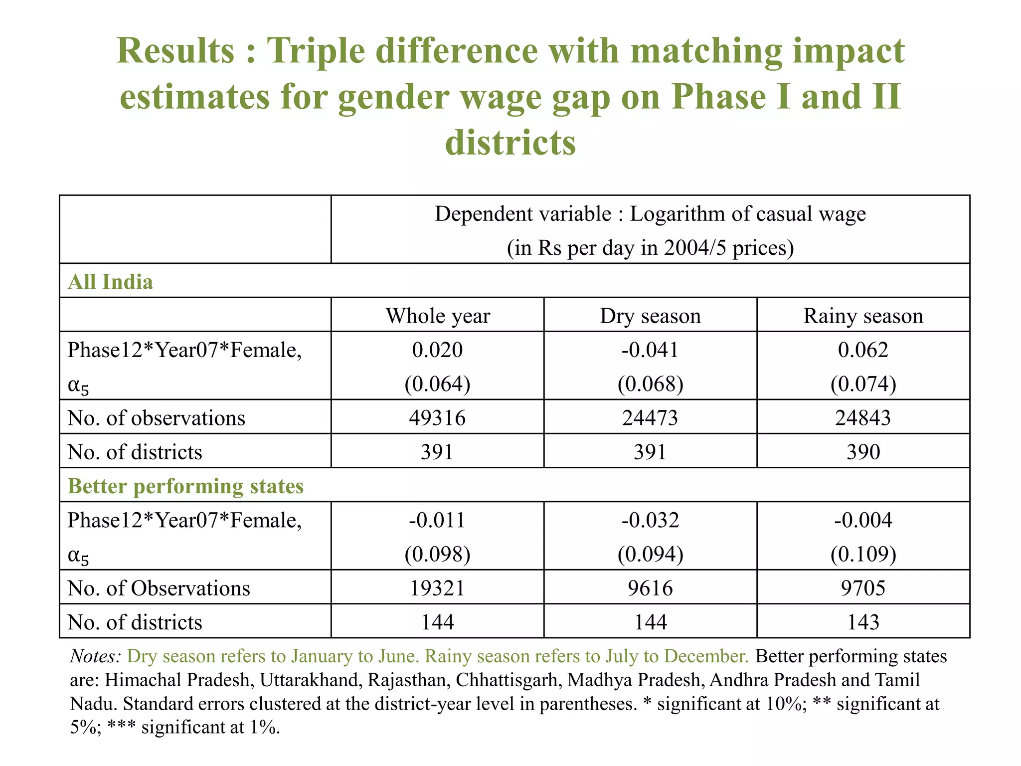
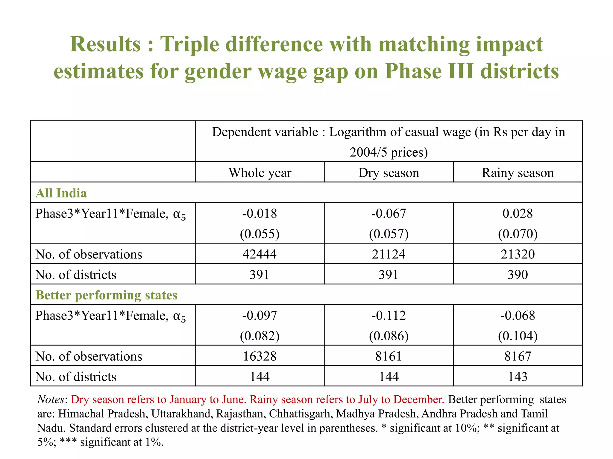
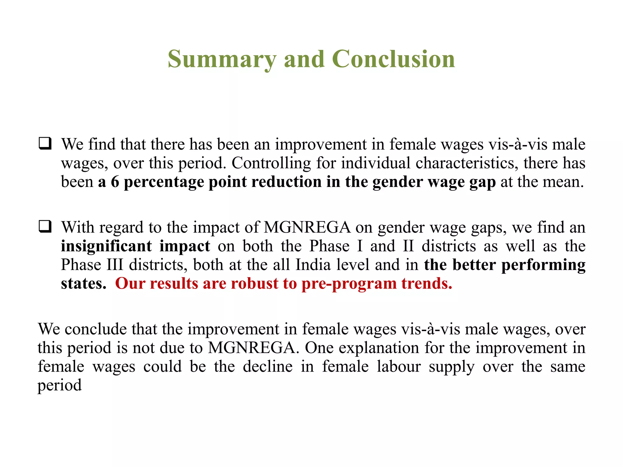

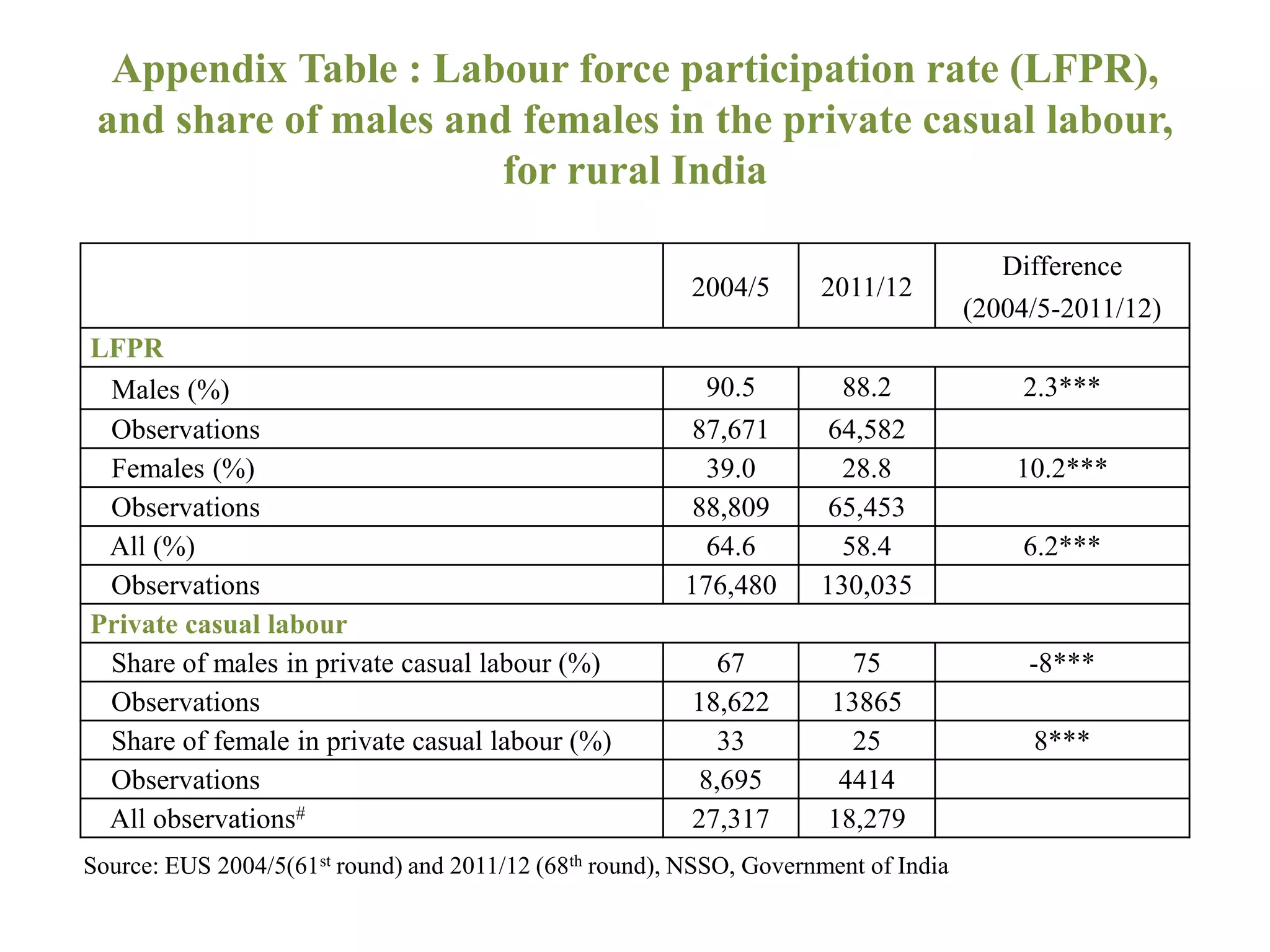
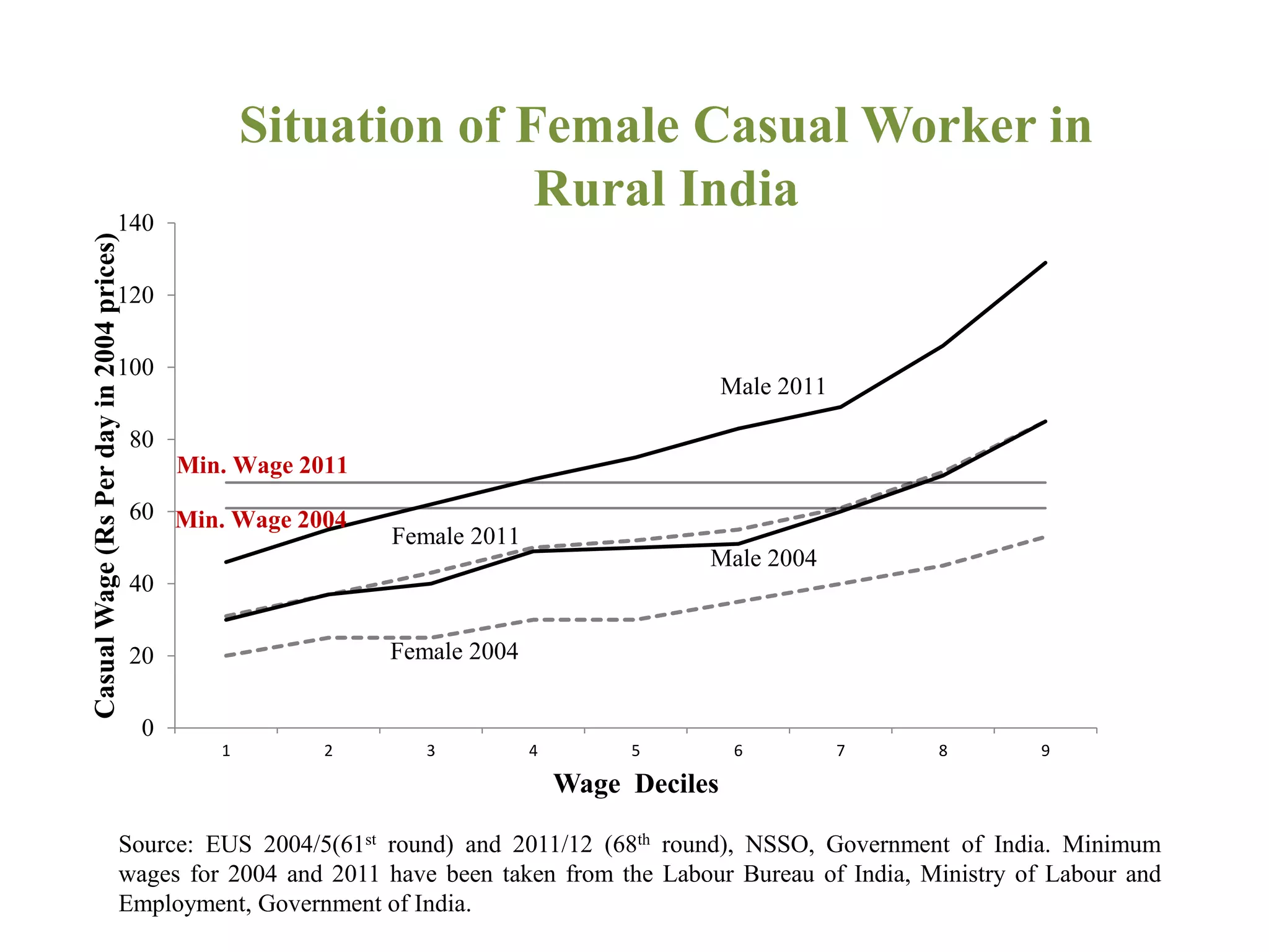
The document analyzes the impact of India's MGNREGA program on reducing gender wage gaps in rural casual labor between 2004-2012. It finds: 1) The gender wage gap declined over this period, with female wages rising 6% relative to male wages on average, after controlling for individual characteristics. 2) However, the analysis using a triple difference matching model finds no significant impact of MGNREGA on further reducing gender wage gaps in either Phase I/II districts where it launched earlier or Phase III districts where it launched later. 3) The improvement in female wages relative to male wages over this time appears to not be caused by MGNREGA. A potential explanation is a decline in


