Statistics Foundation withR
2
PROGRAMME DESIGN COMMITTEE
COURSE DESIGN COMMITTEE
COURSE PREPARATION TEAM
PRINT PRODUCTION
Copyright Reserved 2025
All rights reserved. No Part of this publication which is material protected by this
copy right notice may be reproduced or transmitted or utilized or stored in any
form or by any means, now known or hereinafter invented electronic digital or
mechanical including photocopying scanning, recording or by any information
storage or retrieval system without prior permission from the publisher.
Information contained in this book has been obtained by its Authors from sources
believed to be reliable and are correct to the best of their knowledge. However,
the Publishers and its Authors shall in no event be liable for any errors omissions
or damages arising out of use of this information and specifically disclaim any
implied warranties or merchantability or fitness for any particular use.
3.
Statistics Foundation withR
3
STATISTICS FOUNDATION WITH R
Unit - 1 Introduction To R And Descriptive Statistics.............................. 4
Unit - 2 Statistical Inference: Estimation And Hypothesis Testing ........ 50
Unit - 3 Correlation, Introduction To Regression, And Statistical
Reporting............................................................................................... 103
4.
Statistics Foundation withR
4
UNIT - 1 INTRODUCTION TO R AND
DESCRIPTIVE STATISTICS
STRUCTURE
1.0 Objectives
1.1 Introduction to R and RStudio
1.2 Basic R Syntax and Working with RStudio
1.2.1 R as a Calculator and Variable Assignment
1.2.2 RStudio Interface and Package Management
1.3 R Data Types and Structures
1.4 Vectors, Matrices, and Data Frames
1.5 Importing, Exporting, and Cleaning Data
1.6 Descriptive Statistics
1.7 Data Visualization with R
1.8 Introduction to Probability
1.9 Let Us Sum Up
1.10 Key Words
1.11 Answer To Check Your Progress
1.12 Some Useful Books
1.13 Terminal Questions
1.0 OBJECTIVES
• Understand the functionalities of R and RStudio for statistical computing.
• Apply basic R syntax, data structures, and operations.
• Perform data manipulation tasks using R, including data cleaning and
transformation.
• Calculate and interpret descriptive statistics using R.
• Visualize data effectively using R's built-in plotting functions and
ggplot2.
• Understand fundamental concepts in probability and probability
distributions.
5.
Statistics Foundation withR
5
1.1 INTRODUCTION TO R AND RSTUDIO
The Framework of Statistical Analysis
Statistical analysis is the systematic discipline of transforming raw data
into meaningful insights, providing a rigorous framework for
interpretation and evidence-based decision-making.
Its application can be broadly categorized into two main branches:
• Descriptive Statistics: This involves summarizing and describing the
primary features of a dataset. Through measures of
central tendency (e.g., mean, median) and dispersion (e.g., standard
deviation, range), we can distill complex data into understandable
summaries.
• Inferential Statistics: This is the process of drawing conclusions
about a broader population based on data gathered from a smaller,
representative sample. It allows researchers to test formal hypotheses
about population characteristics and to estimate unknown parameters
with a calculated degree of confidence.
Ultimately, whether describing a sample or making inferences about a
population, the goal is to move beyond mere numbers and uncover the
story the data tells, enabling valid and reliable conclusions.
R and RStudio: The Environment for Modern Data Analysis
To effectively execute these analytical methods, this course utilizes the R
software environment. R is a powerful, open-source programming
language specifically engineered for the complex demands of statistical
computing and graphical representation. Its open-source nature means it is
freely available and constantly being improved by a global community of
academics and data scientists, ensuring it remains at the forefront of
statistical methodology.
While R provides the underlying computational engine, RStudio serves as
a sophisticated and user-friendly Integrated Development Environment
(IDE). It significantly enhances the R experience by providing a structured
interface that organizes the workflow into logical panes for writing code,
6.
Statistics Foundation withR
6
executing commands, viewing variables, and managing outputs like plots
and files.
The paramount strength of R is its extensive ecosystem of user-contributed
packages, which function as add-ons that provide specialized tools for a
virtually unlimited range of tasks—from advanced statistical modeling
and machine learning to bioinformatics and econometrics. This makes R
an incredibly versatile and adaptable tool for modern research.
Course Approach: Integrating Theory with Application
This unit is designed to meticulously bridge the gap between abstract
statistical theory and its concrete, practical application using R. The
learning process will guide you through a complete and realistic data
analysis workflow. This encompasses the essential skills of importing data
from various sources (like CSV or Excel files), performing necessary data
cleaning and transformation, executing appropriate statistical tests, and
producing high-quality, publication-ready visualizations to communicate
findings effectively.
A central tenet of this approach is fostering reproducible research. By
using R and RStudio, you will learn to create analyses that are transparent,
verifiable, and easily shared, ensuring the integrity and credibility of your
work. This hands-on methodology will equip you not just with theoretical
knowledge, but with the robust, practical skills required to confidently
tackle real-world data challenges
1.2 BASIC R SYNTAX AND WORKING WITH RSTUDIO
This section provides a comprehensive overview of the fundamental
syntax of R and introduces the key features of the RStudio IDE. Mastering
the basic syntax is crucial for effectively communicating with the R engine
and writing code that performs the desired statistical analyses. We'll begin
with using R as a basic calculator, demonstrating its ability to perform
simple arithmetic operations. This seemingly simple starting point
illustrates the immediate and interactive nature of the R environment.
From there, we will delve into the crucial concept of variable assignment,
7.
Statistics Foundation withR
7
which is the cornerstone of any programming language. Understanding
how to store and manipulate data using variables is paramount for any R
programming task, as it allows you to create reusable code and perform
complex calculations.
We'll explore the different components of RStudio in detail, highlighting
their individual functionalities and how they work together to create a
seamless development experience. This includes the console for
immediate execution of commands and viewing output, the script editor
for writing, editing, and saving R code in a structured manner, the
environment pane for managing variables and viewing their values, and
the plotting pane for visualizing data and creating graphs. Efficiently
utilizing these components is key to maximizing your productivity and
writing well-organized code.
Furthermore, we will explore how to install and load additional R
packages, which significantly extend R's capabilities beyond its base
functionality. R's package ecosystem is one of its greatest strengths,
providing access to a vast collection of specialized tools for a wide range
of tasks. We will cover the process of installing packages from CRAN
(Comprehensive R Archive Network), the official repository for R
packages, as well as other sources. We will also learn how to effectively
utilize R's built-in help system to find solutions to common problems and
learn more about specific functions and packages. This includes using the
`help()` function, the `?` operator, and searching online resources such as
the R documentation and Stack Overflow.
Specifically, this section will cover the following topics in detail:
● Arithmetic Operations: Performing basic calculations using R's
arithmetic operators (+, -, *, /, ^).
● Variable Assignment: Assigning values to variables using the `<-`,
`=`, and `->` operators.
● Variable Types: Understanding the different data types in R (numeric,
8.
Statistics Foundation withR
8
character, logical, factor, etc.).
● RStudio Interface: Navigating the RStudio interface and utilizing its
key features (console, script editor, environment pane, plotting pane).
● Package Management: Installing, loading, and managing R packages
using the `install.packages()` and `library()` functions.
● Help System: Utilizing R's built-in help system to find information
about functions and packages.
● Working Directory: Setting and managing the working directory in R.
By the end of this section, you will have a solid understanding of R's basic
syntax and the RStudio interface, enabling you to write and execute simple
R code, manage variables, install and load packages, and utilize R's help
system effectively. This will provide a strong foundation for the more
advanced topics covered in subsequent sections.
1.2.1 R as a Calculator and Variable Assignment
R's interactive console functions much like a powerful calculator, allowing
immediate evaluation of arithmetic expressions. This interactive nature is
one of R's key strengths, allowing you to quickly test code snippets and
explore data. For instance, typing `2 + 2` and pressing Enter will
immediately return the result `4`. You can also perform more complex
calculations, such as `(3 * 4) / 2`, which will return `6`. R follows the
standard order of operations (PEMDAS/BODMAS), so parentheses are
used to control the order of evaluation. This immediate feedback makes R
an excellent tool for learning and experimentation.
However, R's true power lies in its ability to store and manipulate data
using variables. Variable assignment involves giving a name to a value,
enabling reuse and manipulation throughout your code. This is a
fundamental concept in programming and is essential for building more
complex analyses. The most common assignment operator is '<-', though
'=' is also acceptable. The `<-` operator is generally preferred in the R
community as it is less ambiguous and avoids potential conflicts with other
9.
Statistics Foundation withR
9
operators. For example, `x <- 5` assigns the value 5 to the variable named
'x'. Now, whenever you type 'x' in the console, R will substitute the value
5. You can then use 'x' in further calculations, such as `x + 3`, which will
return `8`.
Understanding variable types (numeric, character, logical) and appropriate
assignment is fundamental to effective R programming. R is dynamically
typed, meaning you don't need to explicitly declare the type of a variable.
R will automatically infer the type based on the value assigned. However,
it's important to be aware of the different types and how they behave.
Numeric variables can store numbers (integers and decimals), character
variables can store text, and logical variables can store boolean values
(TRUE or FALSE). Using the correct variable type is crucial for
performing accurate calculations and avoiding errors.
The use of descriptive variable names enhances code readability and
maintainability. This is a key principle of good programming practice. For
instance, `average_temperature <- 25` is much more informative than `a
<- 25`. Descriptive variable names make your code easier to understand,
both for yourself and for others who may need to read or modify your code
in the future. Choosing meaningful variable names is an investment that
pays off in the long run.
Here are some examples to illustrate the concepts discussed:
● Example 1: Basic Arithmetic
R
# Addition
2 + 2
# Subtraction
5 - 3
# Multiplication
10.
Statistics Foundation withR
10
4 * 6
# Division
10 / 2
# Exponentiation
2 ^ 3
● Example 2: Variable Assignment
R
# Assigning a numeric value to a variable
my_number <- 10
# Assigning a character value to a variable
my_name <- "Alice"
# Assigning a logical value to a variable
is_raining <- TRUE
● Example 3: Using Variables in Calculations
R
# Assigning values to two variables
width <- 5
height <- 10
# Calculating the area of a rectangle
area <- width * height
# Printing the value of the area variable
area
● Example 4: Descriptive Variable Names
R
11.
Statistics Foundation withR
11
# Using descriptive variable names
annual_interest_rate <- 0.05
principal_amount <- 1000
# Calculating the annual interest
annual_interest <- principal_amount * annual_interest_rate
# Printing the annual interest
annual_interest
In conclusion, understanding how to use R as a calculator and how to
assign values to variables is a fundamental step in learning R
programming. These basic concepts will serve as the foundation for more
advanced topics and will enable you to write more complex and
sophisticated analyses.
1.2.2 RStudio Interface and Package Management
RStudio provides a structured and user-friendly environment for working
with R, significantly enhancing productivity and code organization. The
interface is typically divided into four main panes, each serving a specific
purpose. Understanding the functionality of each pane is crucial for
efficient R programming. The console is the interactive window for
immediate code execution. Here, you can type R commands and see the
results immediately. It's useful for quick calculations, testing code
snippets, and exploring data. However, it's not ideal for writing and saving
larger programs.
The script editor allows you to write and save R code in a text file,
facilitating reproducible research and collaboration. This is where you'll
spend most of your time writing and editing your R programs. The script
editor provides features such as syntax highlighting, code completion, and
error checking, which make coding easier and less prone to errors. You
12.
Statistics Foundation withR
12
can save your scripts as '.R' files and execute them by clicking the 'Run'
button or using keyboard shortcuts.
Fig:1.1 R Studio Interface
The environment pane displays the currently defined variables and their
values, providing a clear overview of your workspace. This is extremely
useful for tracking the variables you've created and their current values. It
helps you avoid errors caused by using the wrong variable or accidentally
overwriting a variable. You can also import datasets directly into your
environment from this pane.
The plots pane displays graphical outputs generated by R's plotting
functions. This is where you'll see the charts and graphs you create using
R's built-in plotting functions or packages like ggplot2. You can also
export plots to various formats for use in reports and presentations.
Efficient use of RStudio's features significantly improves workflow,
allowing you to write, execute, debug, and visualize your code in a
streamlined manner.
13.
Statistics Foundation withR
13
R's functionality is greatly expanded through packages, which are
collections of functions, data, and documentation that extend R's
capabilities beyond its base functionality. Packages are contributed by
users and developers from around the world and cover a wide range of
topics, from statistical modeling to data visualization to machine learning.
The `install.packages()` function is used to install new packages from
CRAN (Comprehensive R Archive Network) or other repositories. CRAN
is the official repository for R packages and is the most common source
for installing packages. The `library()` function loads a package, making
its functions accessible in your current R session. Once a package is
loaded, you can use its functions just like any other R function.
For instance, to install the `ggplot2` package, a popular package for
creating beautiful and informative visualizations, you would use the
following command in the console:
R
install.packages("ggplot2")
After the package is successfully installed, you need to load it into your R
session using the `library()` function:
R
library(ggplot2)
Now you can use the functions provided by the `ggplot2` package to create
plots. Here are some additional examples to illustrate package
management and RStudio interface:
Example 1: Installing and Loading a Package
R
# Installing the dplyr package (for data manipulation)
install.packages("dplyr")
# Loading the dplyr package
14.
Statistics Foundation withR
14
library(dplyr)
Example 2: Using Functions from a Package
R
# Loading the dplyr package
library(dplyr)
# Creating a data frame
data <- data.frame(x = 1:5, y = c(2, 4, 6, 8, 10))
# Using the filter() function from dplyr to filter the data frame
filtered_data <- filter(data, y > 5)
# Printing the filtered data
filtered_data
Example 3: Exploring the RStudio Interface
1. Console: Type `2 + 2` in the console and press Enter to see the result.
2. Script Editor: Create a new R script file (File -> New File -> R Script),
write some R code, and save the file with a '.R' extension.
3. Environment Pane: Create some variables (e.g., `x <- 5`, `y <-
"hello"`) and observe how they appear in the environment pane.
4. Plots Pane: Create a simple plot (e.g., `plot(1:10)`) and observe how it
appears in the plots pane.
15.
Statistics Foundation withR
15
Fig:1.2 R-Studio Interface
By mastering the RStudio interface and understanding how to install and
load packages, you'll be well-equipped to tackle a wide range of data
analysis tasks in R. These skills are essential for any aspiring data scientist
or statistician using R.
Check Your Progress -1
1. What is the primary difference between R and RStudio?
.....................................................................................................................
.....................................................................................................................
2. Explain the purpose of the 'install. Packages()' and 'library()' functions.
.....................................................................................................................
.....................................................................................................................
3. Describe the function of the four main panes in RStudio.
.....................................................................................................................
.....................................................................................................................
16.
Statistics Foundation withR
16
1.3 R DATA TYPES AND STRUCTURES
Understanding data types and structures is foundational to effective data
analysis in R. R, unlike some other programming languages, is a
dynamically typed language, which means you don't need to declare the
type of a variable explicitly. R infers the type based on the value assigned
to it. This flexibility, however, necessitates a strong understanding of the
underlying data types to avoid unexpected behavior and ensure the
integrity of your analysis. Let's delve into the core data types and structures
in R.
Data Types
R supports several fundamental data types, each designed to represent
different kinds of information:
• Numeric: This type represents real numbers, which include both
integers and decimal values. Examples include `3.14`, `-2.5`, and `0`.
Under the hood, R often stores numeric values as double-precision
floating-point numbers for maximum precision. However, this can
sometimes lead to unexpected behavior due to the limitations of
floating-point representation. For example, adding two numbers that
should theoretically result in a simple integer might yield a slightly
different floating-point value due to rounding errors.
Example: x <- 3.14; typeof(x)` will return "double".
• Integer: This type represents whole numbers without any decimal
component. Examples include `1`, `10`, and `-5`. While R
automatically treats whole numbers as numeric, you can explicitly
declare an integer using the `L` suffix. Using integers can be more
memory-efficient when dealing with large datasets consisting only of
whole numbers.
Example: y <- 10L; typeof(y)` will return "integer".
• Character: This type represents text strings. Character strings are
enclosed in single or double quotes (e.g., "Hello", 'R'). Character data
is used for storing names, labels, and any other textual information. R
17.
Statistics Foundation withR
17
provides a rich set of functions for manipulating character strings,
including functions for searching, replacing, and formatting text.
Example: z <- "Hello"; typeof(z)` will return "character".
• Logical: This type represents Boolean values, which can be either
`TRUE` or `FALSE`. Logical values are the result of logical
operations, such as comparisons (`>`, `<`, `==`) or logical operators
(`&`, `|`, `!`). Logical values are fundamental for controlling the flow
of execution in your R scripts using conditional statements (e.g., `if`,
`else`) and for filtering data based on specific criteria.
Example: a <- TRUE; typeof(a)` will return "logical". `b <- (5 > 3);
print(b)` will output `TRUE`.
• Factor: This type represents categorical data. Factors are used to
represent variables that take on a limited number of distinct values,
often representing groups or categories. Examples include gender
(male, female), education level (high school, bachelor's, master's), or
treatment group (control, treatment). Factors are crucial for statistical
modeling because they allow R to treat categorical variables
appropriately in statistical analyses. Factors have two key components:
a vector of integer values representing the levels and a set of labels
associated with each level. This representation allows R to efficiently
store and process categorical data.
Example: gender <- factor(c("male", "female", "male"));
typeof(gender)` will return "integer". The levels can be accessed using
`levels(gender)`.
Data Structures
R provides several data structures for organizing and storing data. These
structures differ in terms of their dimensionality, the types of data they can
hold, and the operations that can be performed on them.
Vectors: Vectors are the most basic data structure in R. A vector is a one-
dimensional array that holds a sequence of elements of the same data type.
You can create vectors using the `c()` function (concatenate).
18.
Statistics Foundation withR
18
Example: numeric_vector <- c(1, 2, 3, 4, 5)`;
character_vector <- c("a", "b", "c")`.
Attempting to create a vector with mixed data types will result in coercion,
where R automatically converts all elements to the most general data type
(e.g., converting numbers to characters if a character element is present).
Matrices: Matrices are two-dimensional arrays. A matrix is a collection
of elements of the same data type arranged in rows and columns. You can
create matrices using the `matrix()` function, specifying the data, the
number of rows, and the number of columns.
Example: `matrix_data <- matrix(1:9, nrow = 3, ncol = 3)`.
This creates a 3x3 matrix with the numbers 1 through 9. Matrices are
fundamental for linear algebra operations and are used extensively in
statistical modeling.
Arrays: Arrays are multi-dimensional generalizations of matrices. While
matrices are limited to two dimensions, arrays can have any number of
dimensions. You can create arrays using the `array()` function, specifying
the data and the dimensions.
Example: array_data <- array(1:24, dim = c(2, 3, 4)).
This creates a three-dimensional array with dimensions 2x3x4.
Lists: Lists are highly flexible data structures that can hold elements of
different data types. A list can contain numbers, characters, logical values,
vectors, matrices, and even other lists. You can create lists using the `list()`
function.
Example: my_list <- list(name = "John", age = 30, scores = c(85, 90, 92)).
Lists are useful for storing complex data structures and for returning
multiple values from a function.
Data Frames: Data frames are tabular data structures that are similar to
spreadsheets or SQL tables. A data frame is a collection of columns, each
19.
Statistics Foundation withR
19
of which is a vector. All columns in a data frame must have the same
length, but they can have different data types. Data frames are the
workhorse of R for data analysis. You can create data frames using the
`data.frame()` function.
Example: `my_data <- data.frame(name = c("John", "Jane"), age = c(30,
25), city = c("New York", "London"))`.
The `dplyr` package provides powerful tools for manipulating data frames,
including functions for filtering, sorting, and transforming data.
Coercion
As mentioned earlier, R performs coercion when you try to combine
different data types in a vector or matrix. R automatically converts
elements to the most general data type to ensure consistency.
The order of coercion is typically logical -> integer -> numeric ->
character.
This means that if you combine a logical value with a numeric value, the
logical value will be converted to numeric (TRUE becomes 1, FALSE
becomes 0). If you combine a numeric value with a character value, the
numeric value will be converted to character.
Understanding data types and structures is essential for writing efficient
and effective R code. By choosing the appropriate data type and structure
for your data, you can optimize memory usage, improve performance, and
ensure the accuracy of your analysis.
Check Your Progress - 2
1. What is the difference between a numeric and an integer data type in R?
.....................................................................................................................
.....................................................................................................................
2. What is the most common data structure used in R for data analysis, and
why?
.....................................................................................................................
20.
Statistics Foundation withR
20
.....................................................................................................................
3. Explain the difference between a vector and a list in R.
.....................................................................................................................
.....................................................................................................................
1.4 VECTORS, MATRICES, AND DATA FRAMES
Vectors, matrices, and data frames are fundamental data structures in R,
each serving distinct purposes in data manipulation and analysis.
Understanding their properties and operations is crucial for effective data
handling. Let's explore each of these structures in detail.
Vectors
Vectors are the most basic building blocks in R. They are one-dimensional
arrays that hold an ordered sequence of elements of the *same* data type.
This homogeneity is a key characteristic of vectors. Vectors are used to
represent a single variable or a set of related values.
Creation: Vectors are typically created using the `c()` function, which
stands for "concatenate." This function combines individual elements into
a vector.
Example: `my_vector <- c(1, 2, 3, 4, 5)` creates a numeric vector
containing the numbers 1 through 5. `my_char_vector <- c("a", "b", "c")`
creates a character vector containing the letters a, b, and c.
Indexing: Individual elements in a vector can be accessed using square
brackets `[]`. R uses 1-based indexing, meaning the first element in a
vector has an index of 1.
Example: `my_vector[1]` returns the first element of `my_vector` (which
is 1). `my_vector[3]` returns the third element (which is 3).
You can also use negative indexing to exclude elements. For example,
`my_vector[-1]` returns all elements of `my_vector` except the first
element.
21.
Statistics Foundation withR
21
● Vector Operations: R supports element-wise operations on vectors.
This means that when you perform an operation on two vectors, the
operation is applied to corresponding elements in the vectors.
Example: `vector1 <- c(1, 2, 3); vector2 <- c(4, 5, 6);
result <- vector1 + vector2`.
The `result` vector will be `c(5, 7, 9)`, because 1+4=5, 2+5=7, and 3+6=9.
If the vectors have different lengths, R applies a recycling rule, where the
shorter vector is repeated until it matches the length of the longer vector.
This can be useful in some cases, but it can also lead to unexpected results
if you're not careful.
Example: `vector3 <- c(1, 2); vector4 <- c(3, 4, 5, 6); result2 <- vector3 +
vector4`. `vector3` will be recycled to `c(1, 2, 1, 2)`, and the `result2`
vector will be `c(4, 6, 6, 8)`. This recycling behavior can be controlled
using functions like `rep()` for explicit repetition.
Matrices
Matrices are two-dimensional arrays. They are collections of elements of
the same data type arranged in rows and columns. Matrices are used to
represent tables of data or to perform linear algebra operations.
● Creation: Matrices are created using the `matrix()` function, which
takes the data, the number of rows (`nrow`), and the number of columns
(`ncol`) as arguments.
Example: `my_matrix <- matrix(1:9, nrow = 3, ncol = 3)` creates a 3x3
matrix with the numbers 1 through 9.
By default, the matrix is filled column-wise. You can change this behavior
by specifying `byrow = TRUE`.
Indexing: Elements in a matrix are accessed using two indices: one for the
row and one for the column. The syntax is `matrix[row, column]`.
Example: `my_matrix[1, 1]` returns the element in the first row and first
column. `my_matrix[2, 3]` returns the element in the second row and third
column.
22.
Statistics Foundation withR
22
You can also use slicing to access entire rows or columns. For example,
`my_matrix[1,]` returns the first row, and `my_matrix[, 3]` returns the
third column.
Matrix Operations: R supports a wide range of matrix operations,
including addition, subtraction, multiplication, and transposition.
Example: matrix1 <- matrix(1:4, nrow = 2);
matrix2 <- matrix(5:8, nrow = 2);
matrix_sum <- matrix1 + matrix2` performs element-wise
addition of the two matrices.
matrix_product <- matrix1 %*% matrix2` performs matrix
multiplication.
The `t()` function transposes a matrix, swapping its rows and columns.
Data Frames
Data frames are the workhorse of R for data analysis. They are tabular data
structures that are similar to spreadsheets or SQL tables. A data frame is a
collection of columns, each of which is a vector. All columns in a data
frame must have the same length, but they can have *different* data types.
This flexibility makes data frames ideal for storing real-world datasets,
which often contain a mix of numeric, character, and logical data.
● Creation: Data frames are created using the `data.frame()` function,
which takes named vectors as arguments. Each vector becomes a column
in the data frame.
Example: `my_data <- data.frame(name = c("John", "Jane"), age = c(30,
25), city = c("New York", "London"))` creates a data frame with three
columns: `name` (character), `age` (numeric), and `city` (character).
● Accessing Columns: Columns in a data frame can be accessed using the
`$` operator or using square brackets `[]`.
Example: `my_data$name` returns the `name` column. `my_data["age"]`
also returns the `age` column. `my_data[, 1]` returns the first column.
23.
Statistics Foundation withR
23
● Subsetting Rows: Rows in a data frame can be subsetted using square
brackets `[]` and logical conditions.
Example: `my_data[my_data$age > 25,]` returns all rows where the `age`
is greater than 25.
● Data Manipulation with dplyr: The `dplyr` package provides a
powerful and consistent set of verbs for data manipulation. Some of the
most commonly used functions include:
`select()`: Selects specific columns from a data frame.
Example: `dplyr::select(my_data, name, age)` selects the `name` and
`age` columns.
`filter()`: Filters rows based on a logical condition.
Example: `dplyr::filter(my_data, city == "New York")` filters the data
frame to include only rows where the `city` is "New York".
`mutate()`: Creates new variables or modifies existing variables.
Example: `dplyr::mutate(my_data, age_next_year = age + 1)` creates a
new column called `age_next_year` that contains the age plus 1.
arrange()`: Sorts rows based on one or more columns.
Example: `dplyr::arrange(my_data, age)` sorts the data frame by age in
ascending order.
`summarize()`: Calculates summary statistics for one or more variables.
Example: `dplyr::summarize(my_data, mean_age = mean(age))`
calculates the mean age.
Data frames are the foundation for most data analysis tasks in R. Their
flexibility and the availability of powerful manipulation tools like `dplyr`
make them an essential tool for any data scientist or statistician.
Check Your Progress - 3
1. What is the difference between a numeric and an integer data type in R?
.....................................................................................................................
.....................................................................................................................
24.
Statistics Foundation withR
24
2. What is the most common data structure used in R for data analysis, and
why?
.....................................................................................................................
.....................................................................................................................
3. Explain the difference between a vector and a list in R.
.....................................................................................................................
.....................................................................................................................
1.5 IMPORTING, EXPORTING, AND CLEANING DATA
Efficient data import and export are foundational to robust data analysis
workflows. R, with its rich ecosystem of packages, provides a
comprehensive suite of tools for handling various data formats. The base
R installation includes functions like `read.csv()` and `write.csv()` which
are essential for dealing with comma-separated value (CSV) files, a
ubiquitous format for data exchange due to its simplicity and compatibility
across different platforms. Beyond CSV files, the `readxl` package
significantly extends R's capabilities by enabling seamless import of data
from Excel spreadsheets, accommodating both `.xls` and `.xlsx` formats.
Data import functions offer numerous options to handle encoding issues,
specify delimiters, manage header rows, and control how missing values
are interpreted.
In-Depth Look at Data Import Functions:
read.csv(): This function is highly configurable, allowing users to specify
the delimiter (e.g., comma, tab, semicolon), handle missing values (e.g.,
`NA`, empty strings), and manage text encoding.
For instance, `read.csv("data.csv", header = TRUE, sep = ",", na.strings =
c("", "NA"))` reads a CSV file, treats the first row as headers, uses a
comma as the delimiter, and interprets both empty strings and "NA" as
missing values.
25.
Statistics Foundation withR
25
read_excel(): From the `readxl` package, this function simplifies
importing data from Excel files. It can read specific sheets within a
workbook and handle different data types seamlessly.
For example, `read_excel("data.xlsx", sheet = "Sheet1")` reads data from
the "Sheet1" sheet of the specified Excel file.
Data cleaning is an indispensable step in the data analysis pipeline. Real-
world datasets often contain inconsistencies, errors, and missing values
that can compromise the validity of any subsequent analysis. R provides
powerful tools for detecting, handling, and correcting these issues.
Handling Missing Values:
Missing values are typically represented as `NA` in R. The `is.na()`
function is used to identify missing values within a dataset. For example,
`is.na(data$column)` returns a logical vector indicating which elements in
the specified column are missing.
Removal of missing values can be achieved using functions like
`na.omit()`, which removes rows containing any missing values. However,
this approach should be used cautiously as it can lead to a significant
reduction in sample size and potentially introduce bias. For example,
`na.omit(data)` removes all rows with any `NA` values.
Imputation involves replacing missing values with estimated values.
Common methods include mean imputation (replacing missing values
with the mean of the non-missing values in the column), median
imputation (using the median), or more sophisticated techniques like
regression imputation or multiple imputation.
For instance, to replace missing values in a column with the mean, you can
use: `data$column[is.na(data$column)] <- mean(data$column, na.rm =
TRUE)`. The `na.rm = TRUE` argument ensures that the mean is
calculated only from the non-missing values.
26.
Statistics Foundation withR
26
Recoding Variables:
Recoding involves transforming existing variables into more suitable
forms for analysis. This can include converting continuous variables into
categorical variables, collapsing categories, or standardizing variable
names.
For example, to recode a variable representing age into age groups, you
can use the ifelse() function or the dplyr::case_when() function:
`data$age_group <- ifelse(data$age < 30, "Young", ifelse(data$age < 60,
"Middle-aged", "Senior"))`.
The `dplyr` package provides powerful tools for recoding variables, such
as mutate() and recode().
For example,
data <- mutate(data, gender = recode(gender, "M" = "Male", "F" =
"Female")) recodes the values in the `gender` column.
Creating New Variables:
Creating new variables often involves combining or transforming existing
ones. This can include calculating new ratios, creating interaction terms,
or generating indicator variables.
For example, to create a new variable representing body mass index
(BMI), you can use:
data$BMI <- data$weight / (data$height^2).
Sorting and Ordering Data:
Sorting and ordering data facilitates analysis by arranging data based on
specific variables. This can be useful for identifying patterns, detecting
outliers, or preparing data for visualization. The `order()` function returns
the indices that would sort a vector, which can then be used to reorder the
data frame.
For example,
data <- data[order(data$age), ] sorts the data frame by age in ascending
order.
Merging and Joining Data:
Efficient data merging and joining are crucial when combining datasets
from multiple sources. R provides functions like `merge()` for performing
27.
Statistics Foundation withR
27
database-style joins. The `dplyr` package offers more flexible and efficient
alternatives, such as `left_join()`, `right_join()`, `inner_join()`, and
`full_join()`. For example, `merged_data <- left_join(data1, data2, by =
"ID")` performs a left join of `data1` and `data2` based on the common
variable "ID".
Example: Suppose you have two datasets: one containing customer
information (ID, name, age) and another containing purchase history (ID,
product, date). You can merge these datasets using a left join to combine
the information for each customer:
R
customer_data <- data.frame(ID = 1:5, name = c("Alice", "Bob",
"Charlie", "David", "Eve"), age = c(25, 30, 22, 40, 35))
purchase_data <- data.frame(ID = c(1, 2, 3, 1, 4), product = c("A",
"B", "C", "D", "E"), date = c("2023-01-01", "2023-02-01", "2023-03-01",
"2023-04-01", "2023-05-01"))
merged_data <- left_join(customer_data, purchase_data, by = "ID")
print(merged_data)
This code merges the two datasets based on the "ID" variable, resulting in
a new dataset containing customer information and their corresponding
purchase history.
Effective data import, export, and cleaning are essential skills for any data
analyst. By mastering these techniques, you can ensure the quality and
reliability of your data, leading to more accurate and meaningful insights.
Check Your Progress - 4
1. How do you handle missing values in R?
.....................................................................................................................
.....................................................................................................................
2. What are some methods for recoding variables in R?
.....................................................................................................................
.....................................................................................................................
3. How would you import data from an Excel file into R?
.....................................................................................................................
.....................................................................................................................
28.
Statistics Foundation withR
28
1.6 DESCRIPTIVE STATISTICS
Descriptive statistics are fundamental tools for summarizing and
describing the main features of a dataset. They provide insights into the
central tendency, dispersion, and shape of a distribution, enabling
researchers to understand the characteristics of their data and draw
meaningful conclusions. Data can be categorized into categorical
(qualitative) and numerical (quantitative) types, each requiring different
statistical measures.
Types of Data:
• Categorical Data: This type of data represents characteristics or
qualities and can be further divided into:
• Nominal Data: Consists of categories with no inherent order or
ranking. Examples include color (e.g., red, blue, green), gender (e.g.,
male, female), or type of fruit (e.g., apple, banana, orange).
• Ordinal Data: Consists of categories with a meaningful order or
ranking. Examples include education level (e.g., high school,
bachelor's, master's), satisfaction ratings (e.g., very dissatisfied,
dissatisfied, neutral, satisfied, very satisfied), or socioeconomic status
(e.g., low, medium, high).
• Numerical Data: This type of data represents quantities and can be
further divided into:
• Interval Data: Has equal intervals between values, but no true zero
point. Examples include temperature in Celsius or Fahrenheit (where
0°C or 0°F does not represent the absence of temperature) and dates.
• Ratio Data: Has equal intervals between values and a true zero point,
indicating the absence of the quantity being measured. Examples
include height, weight, age, income, and temperature in Kelvin (where
0 K represents absolute zero).
29.
Statistics Foundation withR
29
Measures of Central Tendency: These measures describe the center or
typical value of a distribution.
• Mean: The average of all values in the dataset. It is calculated by
summing all values and dividing by the number of values. The
mean is sensitive to outliers. For example, the mean of the numbers
2, 4, 6, 8, and 10 is (2+4+6+8+10)/5 = 6.
• Median: The middle value in the dataset when the values are
arranged in ascending order. If there is an even number of values,
the median is the average of the two middle values. The median is
less sensitive to outliers than the mean. For example, the median
of the numbers 2, 4, 6, 8, and 10 is 6. The median of the numbers
2, 4, 6, 8, 10, and 12 is (6+8)/2 = 7.
• Mode: The value that appears most frequently in the dataset. A
dataset can have no mode (if all values appear only once), one
mode (unimodal), or multiple modes (bimodal, trimodal, etc.). For
example, the mode of the numbers 2, 4, 6, 6, 8, and 10 is 6.
Measures of Dispersion: These measures describe the spread or
variability of a distribution.
• Range: The difference between the maximum and minimum
values in the dataset. It provides a simple measure of the total
spread of the data. For example, the range of the numbers 2, 4, 6,
8, and 10 is 10 - 2 = 8.
• Interquartile Range (IQR): The difference between the 75th
percentile (Q3) and the 25th percentile (Q1). It represents the
spread of the middle 50% of the data and is less sensitive to outliers
than the range. For example, if Q1 = 4 and Q3 = 8, then the IQR is
8 - 4 = 4.
• Variance: The average of the squared deviations from the mean. It
measures the overall variability of the data around the mean. A
higher variance indicates greater spread. The formula for variance
is: σ² = Σ(xᵢ - μ)² / N where xᵢ is each data point, μ is the mean, and
N is the number of data points.
30.
Statistics Foundation withR
30
• Standard Deviation: The square root of the variance. It provides
a more interpretable measure of spread, as it is in the same units as
the original data. The formula for standard deviation is: σ = √σ²
• Coefficient of Variation (CV): The standard deviation divided by
the mean. It is a dimensionless measure of relative variability,
allowing for comparison of variability across datasets with
different units or scales. The formula for the coefficient of
variation is: CV = σ / μ
Shape of a Distribution: The shape of a distribution is described by its
skewness and kurtosis.
• Skewness: Measures the asymmetry of a distribution. A symmetric
distribution has a skewness of 0. A positively skewed distribution
(right-skewed) has a long tail extending to the right, indicating a
concentration of values on the left and a few extreme values on the
right. A negatively skewed distribution (left-skewed) has a long tail
extending to the left, indicating a concentration of values on the
right and a few extreme values on the left.
Fig:1.3 Types of Skewness
• Kurtosis: Measures the tailedness of a distribution. A distribution
with high kurtosis (leptokurtic) has heavy tails and a sharp peak,
indicating a greater concentration of values around the mean and
more extreme values. A distribution with low kurtosis (platykurtic)
has light tails and a flatter peak, indicating a more even distribution
of values. A normal distribution has a kurtosis of 3 (mesokurtic).
31.
Statistics Foundation withR
31
Fig:1.4 Kurtosis
Calculating Descriptive Statistics in R: R provides several functions for
calculating descriptive statistics directly.
• mean(x): Calculates the mean of the vector `x`.
• median(x): Calculates the median of the vector `x`.
• sd(x): Calculates the standard deviation of the vector `x`.
• var(x): Calculates the variance of the vector `x`.
• quantile(x, probs = c(0.25, 0.75)): Calculates the 25th and 75th
percentiles (Q1 and Q3) of the vector `x`.
• range(x): Calculates the range of the vector `x`.
• summary(x): Provides a summary of the main descriptive
statistics (min, Q1, median, mean, Q3, max) for the vector `x`.
Example: Consider a dataset of exam scores for 20 students:
R
scores <- c(75, 80, 68, 92, 85, 78, 90, 82, 70, 76, 88, 84, 95, 79, 81, 86,
73, 89, 77, 91)
# Calculate descriptive statistics
mean_score <- mean(scores) # Mean
median_score <- median(scores) # Median
sd_score <- sd(scores) # Standard deviation
range_score <- range(scores) # Range
iqr_score <- IQR(scores) # Interquartile range
32.
Statistics Foundation withR
32
# Print the results
cat("Mean score:", mean_score, "n")
cat("Median score:", median_score, "n")
cat("Standard deviation:", sd_score, "n")
cat("Range:", range_score, "n")
cat("Interquartile range:", iqr_score, "n")
This code calculates and prints the mean, median, standard deviation,
range, and interquartile range of the exam scores, providing a
comprehensive summary of the dataset's main features.
Understanding descriptive statistics is crucial for interpreting and
summarizing data. By calculating and analyzing these measures,
researchers can gain valuable insights into the characteristics of their data
and make informed decisions based on the evidence.
1.7 DATA VISUALIZATION WITH R
Data visualization is an indispensable component of the data analysis
workflow, serving as a bridge between raw data and actionable insights. It
transcends mere presentation, acting as a powerful tool for exploration,
confirmation, and communication. R, with its rich ecosystem of packages,
offers extensive capabilities for creating a wide array of visualizations,
from simple exploratory plots to complex, publication-ready graphics. The
choice of visualization technique depends heavily on the type of data being
analyzed and the specific questions being addressed.
Basic Plotting Functions: R's base graphics system provides a set of
functions for creating fundamental plot types. These functions, such as
`hist()`, `boxplot()`, `plot()`, and `barplot()`, offer a quick and easy way to
visualize data. For example, `hist()` is used to create histograms, which
display the distribution of numerical data by dividing the data into bins
and showing the frequency of values within each bin. `boxplot()` is used
33.
Statistics Foundation withR
33
to create box plots, which summarize the distribution of numerical data by
showing the median, quartiles, and outliers. `barplot()` is used to create
bar charts, which display the frequency or proportion of categorical data.
`plot()` can be used to create scatter plots, which display the relationship
between two numerical variables.
Fig:1.5 Different types of Plots
Example: Visualizing the distribution of exam scores using a histogram:
R
# Generate some random exam scores
set.seed(123) # for reproducibility
exam_scores <- rnorm(100, mean = 75, sd = 10)
# Create a histogram
hist(exam_scores, main = "Distribution of Exam Scores", xlab =
"Score", col = "lightblue", border = "black")
34.
Statistics Foundation withR
34
In this example, we generate 100 random exam scores following a normal
distribution with a mean of 75 and a standard deviation of 10. The `hist()`
function then creates a histogram of these scores, with the x-axis
representing the score and the y-axis representing the frequency. The
`main` argument specifies the title of the plot, the `xlab` argument
specifies the label for the x-axis, the `col` argument specifies the color of
the bars, and the `border` argument specifies the color of the bar borders.
• ggplot2 Package: The `ggplot2` package, based on the Grammar of
Graphics, provides a more powerful and flexible approach to data
visualization. The Grammar of Graphics is a theoretical framework
that breaks down a plot into its fundamental components: data,
aesthetics, geometries, facets, and statistics.
This allows users to create highly customized and complex plots by
specifying each of these components.
• Data: The dataset to be visualized.
• Aesthetics: The visual attributes of the data, such as position, color,
shape, and size.
• Geometries: The type of mark used to represent the data, such as
points, lines, bars, and boxes.
• Facets: The way to split the data into subsets and create multiple plots.
• Statistics: The statistical transformations to be applied to the data,
such as calculating means and standard deviations.
Example: Creating a scatter plot of height vs. weight using `ggplot2`:
R
library(ggplot2)
# Sample data (replace with your actual data)
height <- c(160, 165, 170, 175, 180)
weight <- c(60, 65, 70, 75, 80)
data <- data. Frame(height, weight)
# Create a scatter plot
ggplot(data, aes(x = height, y = weight)) +
35.
Statistics Foundation withR
35
geom_point() +
labs(title = "Height vs. Weight", x = "Height (cm)", y = "Weight
(kg)") +
theme_minimal()
In this example, we first load the `ggplot2` package. Then, we create a data
frame with two variables: height and weight. The `ggplot()` function
initializes the plot, specifying the data frame and the aesthetic mappings
(x = height, y = weight). The `geom_point()` function adds points to the
plot, creating a scatter plot. The `labs()` function adds a title and axis labels
to the plot. The `theme_minimal()` function applies a minimal theme to
the plot.
● Customization: Customizing plots is essential for enhancing clarity and
aesthetics. This involves adding titles, labels, changing colors, adjusting
themes, and modifying other visual attributes. `ggplot2` provides a wide
range of options for customization, including:
● Titles and labels: The `labs()` function can be used to add titles, axis
labels, and legends to the plot.
● Colors: The `color` and `fill` aesthetics can be used to change the colors
of the plot elements.
The `scale_color_manual()` and `scale_fill_manual()` functions can be
used to specify custom color palettes.
● Themes: The `theme()` function can be used to modify the overall
appearance of the plot. `ggplot2` provides several built-in themes, such as
36.
Statistics Foundation withR
36
`theme_minimal()`, `theme_bw()`, and `theme_classic()`. Custom themes
can also be created.
● Annotations: The `annotate()` function can be used to add annotations
to the plot, such as text, arrows, and rectangles.
Effective Data Visualization: Effective data visualization is critical for
communicating results clearly and persuasively. A well-designed
visualization can highlight important patterns and trends in the data,
making it easier for the audience to understand the key findings.
Some key principles of effective data visualization include:
● Choosing the right plot type: The choice of plot type should be
appropriate for the type of data being visualized and the specific questions
being addressed.
● Avoiding clutter: The plot should be free of unnecessary clutter, such
as excessive gridlines, labels, and colors.
● Using clear and concise labels: The plot should have clear and concise
titles, axis labels, and legends.
● Highlighting important information: The plot should highlight
important patterns and trends in the data, using techniques such as color,
size, and annotations.
In conclusion, data visualization is a crucial skill for data analysts and
scientists. R provides a powerful and flexible set of tools for creating a
wide range of visualizations, from simple exploratory plots to complex,
publication-ready graphics. By understanding the principles of effective
data visualization and mastering the tools available in R, users can
effectively communicate their findings and insights to a wider audience.
Check Your Progress - 5
1. Explain the purpose and benefits of data visualization in the context of
data analysis.
.....................................................................................................................
.....................................................................................................................
2. Describe the difference between basic plotting functions in R and the
ggplot2 package.
.....................................................................................................................
37.
Statistics Foundation withR
37
.....................................................................................................................
3. Explain the Grammar of Graphics and how it relates to the ggplot2
package.
.....................................................................................................................
.....................................................................................................................
4. List and explain at least three ways to customize plots in R to enhance
clarity and aesthetics.
.....................................................................................................................
.....................................................................................................................
5. What are some key principles of effective data visualization?
.....................................................................................................................
.....................................................................................................................
1.8 INTRODUCTION TO PROBABILITY
Probability theory is the mathematical framework that allows us to
quantify and reason about uncertainty. It provides the foundation for
statistical inference, enabling us to make informed decisions based on data,
even when the outcomes are not perfectly predictable. Understanding
probability is essential for interpreting statistical results and drawing
meaningful conclusions.
Probability Experiment: A probability experiment is any process or
trial that results in an uncertain outcome. This outcome cannot be predicted
with certainty before the experiment is conducted. Probability experiments
form the basis for studying random phenomena. Examples include:
• Tossing a coin: The outcome is either heads or tails, which is uncertain
before the toss.
• Rolling a die: The outcome is a number from 1 to 6, which is uncertain
before the roll.
• Drawing a card from a deck: The outcome is a specific card, which
is uncertain before the draw.
38.
Statistics Foundation withR
38
• Measuring the height of a randomly selected person: The outcome
is a numerical value, which is uncertain before the measurement.
Sample Space: The sample space, denoted by 'S', is the set of all possible
outcomes of a probability experiment. Each outcome in the sample space
is called a sample point. For example:
If the experiment is tossing a coin, the sample space is S = {Heads, Tails}.
If the experiment is rolling a six-sided die, the sample space is S = {1, 2,
3, 4, 5, 6}.
Event: An event is a subset of the sample space. It represents a specific
outcome or a group of outcomes that we are interested in. Events are
usually denoted by capital letters (e.g., A, B, C). For example, if the
experiment is rolling a die, the event 'rolling an even number' would be
represented by the set {2, 4, 6}.
Basic Rules of Probability:
• The probability of any event must be between 0 and 1, inclusive. That
is, 0 ≤ P(A) ≤ 1 for any event A.
• The probability of the sample space (i.e., the probability that some
outcome occurs) is 1. That is, P(S) = 1.
• If two events A and B are mutually exclusive (i.e., they cannot occur
at the same time), then the probability of their union (i.e., the
probability that either A or B occurs) is the sum of their individual
probabilities. This is known as the addition rule: P(A ∪ B) = P(A) +
P(B).
• If two events A and B are independent (i.e., the occurrence of one does
not affect the probability of the other), then the probability of their
intersection (i.e., the probability that both A and B occur) is the product
of their individual probabilities. This is known as the multiplication
rule: P(A ∩ B) = P(A) * P(B).
Discrete Probability Distributions: A discrete probability distribution
assigns probabilities to distinct, countable outcomes. Each outcome has a
specific probability associated with it, and the sum of all probabilities must
equal 1. A classic example is the binomial distribution, which models the
39.
Statistics Foundation withR
39
probability of obtaining a certain number of successes in a fixed number
of independent trials, where each trial has only two possible outcomes
(success or failure).
Example: Binomial Distribution
Consider an experiment where you flip a coin 10 times (n = 10), and you
want to find the probability of getting exactly 6 heads (k = 6), assuming
the coin is fair (p = 0.5).
The probability mass function (PMF) for the binomial distribution is given
by:
P(X = k) = C(n, k) * p^k * (1 - p)^(n - k)
Where:
P(X = k) is the probability of getting k successes in n trials.
C(n, k) is the number of combinations of n items taken k at a time, also
written as "n choose k".
p is the probability of success on a single trial.
n is the number of trials.
k is the number of successes.
In our case, n = 10, k = 6, and p = 0.5. Plugging these values into the
formula:
P(X = 6) = C(10, 6) * (0.5)^6 * (0.5)^(10 - 6)
First, we calculate C(10, 6):
C(10, 6) = 10! / (6! * (10 - 6)!) = 10! / (6! * 4!) = (10 * 9 * 8 * 7) / (4 * 3
* 2 * 1) = 210
Now, we plug this into the formula:
P(X = 6) = 210 * (0.5)^6 * (0.5)^4 = 210 * (0.015625) * (0.0625) = 210 *
0.0009765625 ≈ 0.205078125
40.
Statistics Foundation withR
40
So, the probability of getting exactly 6 heads in 10 coin flips is
approximately 0.205 or 20.5%.
Continuous Probability Distributions: A continuous probability
distribution assigns probabilities to intervals of outcomes. Unlike discrete
distributions, continuous distributions do not assign probabilities to
individual values; instead, probabilities are associated with ranges of
values. The most prominent example is the normal distribution, also
known as the Gaussian distribution. It is characterized by its bell-shaped
curve and is completely defined by its mean (μ) and standard deviation (σ).
The normal distribution is ubiquitous in statistics due to its mathematical
properties and its tendency to arise naturally in many real- world
phenomena.
Standard Normal Distribution: The standard normal distribution is a
special case of the normal distribution with a mean of 0 and a standard
deviation of 1. It is often denoted by Z. Any normal distribution can be
transformed into the standard normal distribution by subtracting the mean
and dividing by the standard deviation. This transformation is called
standardization.
Z-scores: Z-scores are standardized values that represent the number of
standard deviations a particular value is away from the mean of its
distribution. A positive Z-score indicates that the value is above the mean,
while a negative Z-score indicates that the value is below the mean. Z-
scores allow for comparisons across different normal distributions.
Example: Calculating Z-score
Suppose a student scores 80 on a test. The class average (mean) is 70, and
the standard deviation is 5. Calculate the z-score to understand how well
the student performed compared to the class.
Z = (X - μ) / σ
Z = (80 - 70) / 5
41.
Statistics Foundation withR
41
Z = 10 / 5
Z = 2
A z-score of 2 means that the student's score is 2 standard deviations above
the mean. This indicates the student performed very well compared to their
peers.
Central Limit Theorem (CLT): The Central Limit Theorem (CLT) is
a fundamental concept in statistics. It states that the distribution of sample
means approaches a normal distribution as the sample size increases,
regardless of the shape of the original population distribution. This holds
true even if the population distribution is not normal, provided that the
sample size is sufficiently large (typically, n ≥ 30). The CLT is crucial for
statistical inference because it allows us to make inferences about
population parameters based on sample statistics, even when we don't
know the shape of the population distribution.
In summary, probability theory provides the foundation for understanding
and quantifying uncertainty. Key concepts include probability
experiments, sample spaces, events, basic rules of probability, discrete and
continuous probability distributions, the standard normal distribution, Z-
scores, and the Central Limit Theorem. These concepts are essential for
statistical inference and data analysis.
Check Your Progress - 6
1. Define a probability experiment, sample space, and event. Provide
examples for each.
.....................................................................................................................
.....................................................................................................................
2. State the basic rules of probability, including the addition and
multiplication rules.
.....................................................................................................................
.....................................................................................................................
42.
Statistics Foundation withR
42
3. Explain the difference between discrete and continuous probability
distributions. Provide an example of each.
.....................................................................................................................
.....................................................................................................................
4. What is the standard normal distribution, and why is it important?
.....................................................................................................................
.....................................................................................................................
5. Define Z-scores and explain how they are used.
.....................................................................................................................
.....................................................................................................................
6. State the Central Limit Theorem (CLT) and explain its significance in
statistical inference.
.....................................................................................................................
.....................................................................................................................
1.9 LET US SUM UP
This unit provided a comprehensive introduction to R and descriptive
statistics. We began by exploring the functionalities of R and RStudio,
including installation, basic syntax, data structures, and package
management. We covered essential data manipulation techniques such as
importing, exporting, cleaning, and transforming data. The unit delved
into the calculation and interpretation of descriptive statistics, including
measures of central tendency and dispersion, and explored methods for
visualizing data using R's built-in functions and the powerful `ggplot2`
package. Finally, we introduced fundamental concepts in probability,
including probability rules, discrete and continuous distributions, the
standard normal distribution, z-scores, and the central limit theorem. This
foundation in R programming and descriptive statistics is essential for
further study in statistical inference and more advanced analytical
techniques. The ability to effectively use R for data manipulation and
visualization is a valuable skill in today's data-driven world.
43.
Statistics Foundation withR
43
1.10 KEY WORDS
• R: A programming language and software environment for statistical
computing and graphics.
• RStudio: An integrated development environment (IDE) for R.
• Variable: A named storage location for data.
• Vector: An ordered sequence of elements of the same type.
• Matrix: A two-dimensional array of elements.
• Data Frame: A tabular data structure.
• Descriptive Statistics: Numerical summaries of data.
• Probability: The chance of an event occurring.
• Normal Distribution: A continuous probability distribution.
• Central Limit Theorem: A fundamental theorem in statistics.
1.11 ANSWER TO CHECK YOUR PROGRESS
Refer 1.2 for Answer to check your progress- 1 Q. 1
R is a language and environment for statistical computing, while
RStudio is an integrated development environment (IDE) that provides
a user-friendly interface for working with R, including a console, script
editor, environment pane, and plotting pane, which enhances productivity
and code organization.
Refer 1.2 for Answer to check your progress- 1 Q. 2
The `install.packages()` function is used to install new packages from a
repository like CRAN (Comprehensive R Archive Network). The
`library()` function loads a previously installed package, making its
functions available for use in the current R session. Once loaded, the
functions within the package can be used like any other R function.
Refer 1.2 for Answer to check your progress- 1 Q. 3
The four main panes in RStudio are the console, which allows immediate
44.
Statistics Foundation withR
44
code execution; the script editor, for writing and saving R code; the
environment pane, displaying defined variables and their values; and the
plots pane, which displays graphical outputs.
Refer 1.3 for Answer to check your progress- 2 Q. 1
In R, the numeric data type represents real numbers, including both
integers and decimal values, and is often stored as double-precision
floating-point numbers. The integer data type, on the other hand,
represents whole numbers without any decimal component and can be
explicitly declared using the `L` suffix for memory efficiency.
Refer 1.3 for Answer to check your progress- 2 Q. 2
The most common data structure used in R for data analysis is the data
frame. This is because data frames are tabular data structures that can
hold columns of different data types, similar to spreadsheets or SQL tables,
making them highly versatile for organizing and manipulating real-world
datasets. The `dplyr` package further enhances their utility with powerful
functions for data manipulation.
Refer 1.3 for Answer to check your progress- 2 Q. 3
A vector in R is a one-dimensional array that holds elements of the *same*
data type, while a list is a data structure that can hold elements of
*different* data types. Vectors are created using the `c()` function, and
lists are created using the `list()` function. If you attempt to create a vector
with mixed data types, R will perform coercion to convert all elements to
the most general data type.
Refer 1.4 for Answer to check your progress- 3 Q. 1
The provided text does not contain information about the difference
between numeric and integer data types in R. The text explains vectors,
matrices, and data frames.
45.
Statistics Foundation withR
45
Refer 1.4 for Answer to check your progress- 3 Q. 2
Data frames are the most common data structure used in R for data
analysis. They are flexible, allowing columns to have different data types,
which is ideal for storing real-world datasets. Additionally, the availability
of powerful manipulation tools like dplyr makes them essential for data
scientists and statisticians.
Refer 1.4 for Answer to check your progress- 3 Q. 3
The provided content does not contain information about lists in R.
Therefore, I cannot provide a comparison between vectors and lists based
on the given text. The content focuses on vectors, matrices, and data
frames.
Refer 1.5 for Answer to check your progress- 4 Q. 1
In R, missing values are represented as NA, and the `is.na()` function
identifies them. Removal can be done using `na.omit()`, but it may reduce
sample size and introduce bias. Imputation replaces missing values with
estimates like mean imputation using `data$column[is.na(data$column)]
<- mean(data$column, na.rm = TRUE)` or more sophisticated methods
like regression imputation or multiple imputation.
Refer 1.5 for Answer to check your progress- 4 Q. 2
In R, recoding variables can be achieved using functions like ifelse() or
dplyr::case_when() to convert continuous variables into categorical ones
or collapse categories. The dplyr package also offers powerful tools such
as mutate() and recode() for transforming variable values. These methods
allow for flexible and efficient data transformation to suit specific analysis
needs.
Refer 1.5 for Answer to check your progress- 4 Q. 3
To import data from an Excel spreadsheet into R, you can use the
`read_excel()` function from the `readxl` package. This function allows
you to read data from both `.xls` and `.xlsx` files. For example,
46.
Statistics Foundation withR
46
`read_excel("data.xlsx", sheet = "Sheet1")` reads data from the "Sheet1"
sheet of the specified Excel file. The function simplifies importing data
and can handle different data types seamlessly.
Refer 1.7 for Answer to check your progress- 5 Q. 1
Data visualization serves as a bridge between raw data and actionable
insights, acting as a powerful tool for exploration, confirmation, and
communication. It helps in identifying patterns and trends, making it
easier to understand key findings. Effective visualization involves
choosing the right plot type, avoiding clutter, using clear labels, and
highlighting important information.
Refer 1.7 for Answer to check your progress- 5 Q. 2
R's base graphics system offers basic plotting functions like `hist()`,
`boxplot()`, `plot()`, and `barplot()` for quick data visualization. The
ggplot2 package, based on the Grammar of Graphics, provides a more
powerful and flexible approach, allowing highly customized plots by
specifying data, aesthetics, geometries, facets, and statistics. While basic
functions are easy to use for simple plots, ggplot2 excels in creating
complex and publication-ready graphics with greater control over plot
elements and aesthetics.
Refer 1.7 for Answer to check your progress- 5 Q. 3
The Grammar of Graphics is a theoretical framework that breaks down
a plot into its fundamental components: data, aesthetics, geometries,
facets, and statistics. The ggplot2 package is based on this grammar,
providing a powerful and flexible approach to data visualization. It allows
users to create highly customized and complex plots by specifying each of
these components, offering a structured way to build visualizations.
Refer 1.7 for Answer to check your progress- 5 Q. 4
Customizing plots in R can significantly enhance their clarity and
aesthetics. One way is through adjusting titles and labels using the `labs()`
47.
Statistics Foundation withR
47
function to provide clear context. Another method involves modifying
colors of plot elements with aesthetics like `color` and `fill`, and custom
color palettes via `scale_color_manual()` and `scale_fill_manual()`.
Lastly, the overall appearance can be altered using themes, with built-in
options like `theme_minimal()` or custom themes created with the
`theme()` function.
Refer 1.7 for Answer to check your progress- 5 Q. 5
Key principles of effective data visualization include choosing the right
plot type appropriate for the data and questions, avoiding clutter by
minimizing unnecessary elements, using clear and concise labels for
titles, axes, and legends, and highlighting important information
through color, size, and annotations.
Refer 1.8 for Answer to check your progress- 6 Q. 1
A probability experiment is any process or trial that results in an
uncertain outcome. For example, tossing a coin. The sample space is the
set of all possible outcomes of a probability experiment. For example,
when rolling a six-sided die, the sample space is S = {1, 2, 3, 4, 5, 6}. An
event is a subset of the sample space. For example, when rolling a die, the
event 'rolling an even number' would be represented by the set {2, 4, 6}.
Refer 1.8 for Answer to check your progress- 6 Q. 2
The basic rules of probability state that the probability of any event must
be between 0 and 1, inclusive, and the probability of the sample space is
1. The addition rule states that if two events A and B are mutually
exclusive, then P(A ∪ B) = P(A) + P(B). The multiplication rule states
that if two events A and B are independent, then P(A ∩ B) = P(A) * P(B).
Refer 1.8 for Answer to check your progress- 6 Q. 3
A discrete probability distribution assigns probabilities to distinct,
countable outcomes, like the binomial distribution. Each outcome has a
specific probability, and the sum of all probabilities equals 1. A
48.
Statistics Foundation withR
48
continuous probability distribution assigns probabilities to intervals of
outcomes, such as the normal distribution. Probabilities are associated
with ranges of values rather than individual values.
Refer 1.8 for Answer to check your progress- 6 Q. 4
The standard normal distribution is a special case of the normal
distribution with a mean of 0 and a standard deviation of 1, often denoted
by Z. Its importance lies in its role as a reference point; any normal
distribution can be transformed into the standard normal distribution
through standardization by subtracting the mean and dividing by the
standard deviation. This allows for easy comparison and calculation of
probabilities across different normal distributions using Z-scores.
Refer 1.8 for Answer to check your progress- 6 Q. 5
Z-scores are standardized values that indicate how many standard
deviations a particular value is away from the mean of its distribution. A
positive Z-score means the value is above the mean, while a negative Z-
score means it's below the mean. They are used for comparisons across
different normal distributions by transforming them into a standard
normal distribution.
Refer 1.8 for Answer to check your progress- 6 Q. 6
The Central Limit Theorem (CLT) states that the distribution of sample
means approaches a normal distribution as the sample size increases,
regardless of the shape of the original population distribution. This holds
true even if the population distribution is not normal, provided that the
sample size is sufficiently large (typically, n ≥ 30). The CLT is crucial for
statistical inference because it allows us to make inferences about
population parameters based on sample statistics, even when we don't
know the shape of the population distribution.
49.
Statistics Foundation withR
49
1.12 SOME USEFUL BOOKS
• Crawley, M. J. (2013). The R Book. John Wiley & Sons.
• Everitt, B. S., & Hothorn, T. (2011). An introduction to applied
multivariate analysis with R. Springer.
• Field, A. (2013). Discovering statistics using IBM SPSS statistics.
Sage.
• Ligges, U., & Fox, J. (2018). R and S-PLUS Companion to Applied
Regression. Sage.
• Wickham, H., & Grolemund, G. (2016). R for data science. O'Reilly
Media, Inc.
• Zuur, A. F., Ieno, E. N., Walker, N. J., Saveliev, A. A., & Smith,G. M.
(2009). Mixed effects models and extensions in ecology with R.
Springer.
• Venables, W. N., & Ripley, B. D. (2002). Modern applied statistics
with S-PLUS. Springer.
1.13 TERMINAL QUESTIONS
1. Discuss the advantages and disadvantages of using R for statistical
analysis compared to other software packages.
2. Explain the importance of data cleaning in the context of statistical
analysis and describe different techniques for handling missing data.
3. Compare and contrast different measures of central tendency and
dispersion, highlighting their appropriateness for different types of data.
4. Describe the key principles of the Grammar of Graphics and how they
are implemented in ggplot2.
5. Explain the Central Limit Theorem and its implications for statistical
inference.
6. How can you use R to perform a hypothesis test based on data you have
imported and cleaned?
50.
Statistics Foundation withR
50
UNIT - 2 STATISTICAL INFERENCE:
ESTIMATION AND HYPOTHESIS
TESTING
STRUCTURE
2.0 Objectives
2.1 Introduction to Statistical Inference
2.2 Sampling and Sampling Distributions
2.2.1 Population vs. Sample
2.2.2 Parameters vs. Statistics
2.3 Sampling Distribution of the Mean and Standard Error
2.4 Estimation: Point and Interval Estimation
2.4.1 Confidence Intervals for Population Mean
2.4.2 Confidence Intervals for Population Proportion
2.5 Hypothesis Testing
2.6 Hypothesis Tests for Means
2.7 Analysis of Variance (ANOVA)
2.7.1 Principles of One-Way ANOVA
2.7.2 Interpretation of F-statistic and p-value
2.8 Chi-Squared Tests
2.9 Let Us Sum Up
2.10 Key Words
2.11 Answer to Check Your Progress
2.12 Some Useful Books
2.13 Terminal Questions
2.0 OBJECTIVES
• Understand the concepts of sampling and sampling distributions.
• Apply different methods of estimation and interpret confidence
intervals.
51.
Statistics Foundation withR
51
• Perform and interpret hypothesis tests for means and proportions.
• Apply and interpret Analysis of Variance (ANOVA) and Chi-Squared
tests.
• Critically evaluate assumptions and limitations of statistical tests.
• Utilize R software for performing statistical analyses.
2.1 INTRODUCTION TO STATISTICAL INFERENCE
Statistical inference is the process of drawing conclusions about a
population based on data obtained from a sample. It acts as a crucial
bridge, allowing researchers to extrapolate findings from a smaller group
to a larger one, enabling informed decision-making and evidence-based
conclusions. This field is indispensable across numerous disciplines,
including medicine, economics, engineering, and social sciences, where
understanding population characteristics is vital but direct observation of
the entire population is often impractical or impossible. At its core,
statistical inference utilizes probability theory and statistical models to
quantify the uncertainty associated with these generalizations. It
acknowledges that sample data provides an incomplete picture of the
population and aims to provide measures of confidence in the conclusions
drawn.
This unit focuses on two primary branches of statistical inference:
estimation and hypothesis testing. Estimation deals with approximating
the values of unknown population parameters (e.g., the population mean,
variance, or proportion) using sample statistics. It involves constructing
point estimates, which are single values that represent the best guess for
the parameter, and interval estimates (or confidence intervals), which
provide a range of plausible values within which the parameter is likely to
fall. Different methods of estimation, such as maximum likelihood
estimation (MLE) and method of moments, offer various approaches to
obtaining these estimates, each with its own strengths and weaknesses.
52.
Statistics Foundation withR
52
For example, MLE seeks to find the parameter values that maximize the
likelihood of observing the given sample data, while the method of
moments equates sample moments (e.g., sample mean, sample variance)
to their corresponding population moments and solves for the parameters.
Hypothesis testing, conversely, provides a framework for evaluating
specific claims or hypotheses about population parameters. It involves
formulating a null hypothesis (a statement of no effect or no difference)
and an alternative hypothesis (a statement that contradicts the null
hypothesis). Sample data is then used to calculate a test statistic, which
measures the evidence against the null hypothesis. The probability of
observing a test statistic as extreme as, or more extreme than, the one
calculated, assuming the null hypothesis is true, is known as the p-value.
If the p-value is sufficiently small (typically below a predetermined
significance level, denoted by α), the null hypothesis is rejected in favor
of the alternative hypothesis. Common hypothesis tests include t-tests (for
means), z-tests (for means with known population standard deviation), chi-
squared tests (for categorical data), and F-tests (for variances or comparing
multiple means).
The foundation of statistical inference rests firmly on the principles of
probability and sampling distributions. Because we are making
inferences about a population based on a sample, it is crucial to understand
how sample statistics vary from sample to sample. This variability is
described by the sampling distribution, which represents the probability
distribution of a statistic (e.g., the sample mean) if we were to repeatedly
draw samples from the population. A cornerstone of statistical inference is
the Central Limit Theorem (CLT). The CLT states that, under certain
conditions, the sampling distribution of the sample mean approaches a
normal distribution as the sample size increases, regardless of the shape of
the population distribution. This remarkable result allows us to make
inferences about the population mean even when the population
distribution is unknown, as long as the sample size is sufficiently large.
53.
Statistics Foundation withR
53
The CLT provides a powerful tool for constructing confidence intervals
and conducting hypothesis tests.
However, it's crucial to recognize the assumptions and limitations
underlying statistical inference. The validity of statistical inferences
depends on the quality of the data and the appropriateness of the statistical
methods used. Violations of assumptions, such as non-random sampling
or non-normality (when required), can lead to biased or unreliable
conclusions. Therefore, it's essential to carefully consider the context of
the data and the assumptions of the statistical procedures before drawing
inferences. Furthermore, statistical significance does not necessarily imply
practical significance. A statistically significant result may be too small to
be of practical importance in the real world. This unit will equip you with
the theoretical foundations and practical skills necessary to navigate these
complexities, enabling you to analyze data, interpret results, and draw
meaningful conclusions with a critical and informed perspective. For
instance, in a clinical trial for a new drug, statistical inference is used to
determine whether the drug is effective compared to a placebo.
Researchers collect data on patients in both the treatment and control
groups and use hypothesis testing to assess whether the observed
difference in outcomes is statistically significant. Similarly, in market
research, statistical inference is used to estimate consumer preferences and
predict market trends based on survey data collected from a sample of
consumers.
2.2 SAMPLING AND SAMPLING DISTRIBUTIONS
In statistical inference, understanding the concepts of population and
sample is paramount. The population refers to the entire group of
individuals, objects, or events that are of interest in a study. It is the
complete set about which we want to draw conclusions. Examples of
populations include all registered voters in a country, all students enrolled
in a university, or all manufactured items produced by a factory in a year.
54.
Statistics Foundation withR
54
Due to practical constraints such as cost, time, and accessibility, it is often
impossible or impractical to collect data from the entire population.
Therefore, researchers typically rely on a sample, which is a subset of the
population selected for study. The sample should be carefully chosen to be
representative of the population so that inferences made from the sample
can be generalized to the population with a reasonable degree of accuracy.
The primary goal of sampling is to obtain a subset of the population that
accurately reflects the characteristics of the entire group. This allows
researchers to make inferences about the population based on the
information gathered from the sample. However, it is important to
acknowledge the potential for sampling bias, which occurs when the
sample is not representative of the population, leading to systematic errors
in the inferences. Sampling bias can arise from various sources, such as
selection bias (when certain individuals are more likely to be selected for
the sample than others), non-response bias (when individuals who are
selected for the sample do not participate), and convenience sampling
(when the sample is selected based on ease of access rather than
representativeness).
Parameters and statistics are two key concepts in statistical inference.
Parameters are numerical values that describe characteristics of the
population. Examples of population parameters include the population
mean (μ), the population standard deviation (σ), and the population
proportion (p). Since it is often impossible to measure parameters directly,
they are typically estimated using sample data. Statistics, on the other
hand, are numerical values that describe characteristics of the sample.
Examples of sample statistics include the sample mean (x
̄ ), the sample
standard deviation (s), and the sample proportion (p
̂ ). Statistics are
calculated from the observed data and are used to estimate the
corresponding population parameters. The accuracy of these estimations
depends on the representativeness of the sample and the variability within
the population.
55.
Statistics Foundation withR
55
The process of selecting a sample from a population is crucial for ensuring
the validity of statistical inferences. Random sampling is a fundamental
technique that aims to minimize bias by giving every member of the
population an equal chance of being selected. Simple random sampling
(SRS) is the most basic form of random sampling, where each individual
is selected entirely by chance. Other random sampling methods include
stratified sampling (where the population is divided into subgroups or
strata, and a random sample is selected from each stratum) and cluster
sampling (where the population is divided into clusters, and a random
sample of clusters is selected). The choice of sampling method depends on
the research design, the characteristics of the population, and the available
resources. For instance, stratified sampling is useful when the population
has distinct subgroups that may have different characteristics, while cluster
sampling is useful when the population is geographically dispersed.
The sampling distribution describes the probability distribution of a
statistic when repeated samples are drawn from the population. It provides
insights into how the statistic varies from sample to sample and allows us
to quantify the uncertainty associated with estimating population
parameters. For example, the sampling distribution of the mean describes
the distribution of all possible sample means that could be obtained from
a population. The shape, center, and spread of the sampling distribution
depend on the sample size, the population distribution, and the sampling
method. The Central Limit Theorem (CLT) plays a critical role in
understanding sampling distributions. It states that, under certain
conditions, the sampling distribution of the sample mean approaches a
normal distribution as the sample size increases, regardless of the shape of
the population distribution. This allows us to use the normal distribution
to make inferences about the population mean even when the population
distribution is unknown. Understanding sampling distributions is essential
for constructing confidence intervals and conducting hypothesis tests,
which are the cornerstones of statistical inference. For example, in political
polling, pollsters use random sampling to survey a sample of
56.
Statistics Foundation withR
56
voters and estimate the proportion of voters who support a particular
candidate. The sampling distribution of the sample proportion allows them
to calculate a margin of error, which quantifies the uncertainty associated
with their estimate. Similarly, in quality control, manufacturers use
sampling to inspect a sample of products and determine whether the
production process is meeting quality standards. The sampling distribution
of the sample mean or sample proportion allows them to assess the
variability in product quality and make decisions about whether to adjust
the production process.
2.2.1 Population vs. Sample
The distinction between population and sample is a cornerstone of
statistical inference. The population, in statistical terms, represents the
entire group of individuals, objects, or events that are of interest in a
particular study. It encompasses all possible observations about which we
seek to draw conclusions. Defining the population precisely is the first and
often most critical step in any research endeavor. The definition must be
clear, unambiguous, and relevant to the research question. Examples of
populations are diverse and can include all registered voters in a specific
country during an election year, all patients diagnosed with a particular
disease in a hospital network, or all light bulbs manufactured by a company
in a given month.
Fig: 2.1 Population v/s Sample
57.
Statistics Foundation withR
57
Conversely, a sample is a carefully selected subset of the population.
Due to practical limitations such as cost, time constraints, and
accessibility, it is often infeasible or impossible to collect data from
the entire population. Therefore, researchers rely on samples to gather
information and make inferences about the larger population. The goal
is to select a sample that is representative of the population, meaning
that it accurately reflects the characteristics and diversity of the
population. A representative sample allows researchers to generalize
their findings from the sample to the population with a reasonable
degree of confidence.
For example, if a researcher is interested in studying the average
income of adults in a particular city, the population would be all adults
residing in that city. However, it would be impractical to collect
income data from every adult in the city. Instead, the researcher might
select a sample of 500 adults through a random sampling technique.
The sample data would then be used to estimate the average income of
the entire population of adults in the city. The accuracy of this
estimation depends on how well the sample represents the population.
Inferential statistics is the branch of statistics that focuses on using
data from a sample to make inferences, predictions, or generalizations
about the entire population. The process involves using sample
statistics (e.g., sample mean, sample proportion) to estimate
population parameters (e.g., population mean, population proportion)
and to test hypotheses about the population. The validity of these
inferences depends heavily on the quality of the sample. A biased
sample can lead to misleading inferences and inaccurate conclusions
about the population. Therefore, it is crucial to employ appropriate
sampling techniques to minimize bias and ensure that the sample is as
representative as possible.
A crucial concern is whether the sample accurately represents the
population. A biased sample occurs when certain members of the
58.
Statistics Foundation withR
58
population are systematically over- or under-represented in the sample.
This can lead to inaccurate estimates of population parameters and
flawed conclusions. For instance, if a survey on political preferences
is conducted only among individuals attending a specific political
rally, the resulting sample would likely be biased towards the views of
that particular political party, and the results would not be
representative of the broader population. Methods like random
sampling aim to mitigate this bias by giving each population member
an equal chance of selection. Different types of random sampling
techniques, such as simple random sampling, stratified sampling, and
cluster sampling, are used to ensure that the sample is representative
of the population.
However, even with random sampling, there is inherent variability
between samples. This variability is known as sampling error and
arises because each sample is only a subset of the population and may
not perfectly reflect the characteristics of the entire population.
Sampling distributions address this variability by describing the
distribution of sample statistics (e.g., sample means) that would be
obtained if we were to repeatedly draw samples from the same
population. Understanding sampling distributions is essential for
quantifying the uncertainty associated with statistical inferences and
for constructing confidence intervals and conducting hypothesis tests.
For instance, in opinion polls, the margin of error reflects the
uncertainty due to sampling variability and indicates the range within
which the true population parameter is likely to fall. Therefore, the
careful selection of a sample and a thorough understanding of sampling
distributions are essential for making valid and reliable inferences
about the population.
2.2.2 Parameters vs. Statistics
Parameters and statistics are fundamental concepts in statistical
inference, representing numerical summaries used to describe
59.
Statistics Foundation withR
59
characteristics of populations and samples, respectively. However,
their scope, nature, and usage differ significantly. Parameters
describe characteristics of the population, which, as previously
defined, is the entire group of individuals, objects, or events of interest.
Parameters are typically fixed, albeit usually unknown, values. They
represent the true values that we aim to estimate or infer using sample
data. Examples of population parameters include the population mean
(μ), which represents the average value of a variable in the entire
population; the population standard deviation (σ), which measures the
spread or variability of the data in the population; and the population
proportion (p), which represents the fraction of individuals in the
population that possess a certain characteristic.
For instance, consider the task of determining the average height of all
women in a country. The true average height of all women in that
country is a population parameter. Since it is practically impossible
to measure the height of every woman in the country, this parameter
remains unknown. Similarly, if we are interested in the proportion of
voters in a city who support a particular political candidate, the true
proportion of all voters in the city who support the candidate is a
population parameter. These parameters are fixed values that describe
the entire population, but they are typically unknown and need to be
estimated from sample data.
Statistics, on the other hand, describe characteristics of a sample,
which is a subset of the population. Statistics are calculated from
observed data and vary from sample to sample. They are used to
estimate population parameters and to test hypotheses about them.
Examples of sample statistics include the sample mean (x
̄ ), which
represents the average value of a variable in the sample; the sample
standard deviation (s), which measures the spread or variability of the
data in the sample; and the sample proportion (p
̂ ), which represents the
60.
Statistics Foundation withR
60
fraction of individuals in the sample that possess a certain
characteristic.
Fig :2.2 Parameter v/s Statistic
For example, if we randomly select a sample of 100 women from the
country and measure their heights, the sample average height of these 100
women is a sample statistic. This statistic is calculated from the observed
data and varies depending on which 100 women are selected for the
sample. Similarly, if we survey a sample of 500 voters in the city and ask
them whether they support the political candidate, the sample proportion
of voters who support the candidate is a sample statistic. These statistics
are calculated from the sample data and are used to estimate the
corresponding population parameters.
Statistical inference employs sample statistics to estimate population
parameters and test hypotheses about them. The goal is to use the
information contained in the sample to make inferences about the larger
population. This process inherently involves uncertainty, as the sample is
only a subset of the population and may not perfectly reflect the
characteristics of the entire population. The difference between parameters
and statistics is crucial because our inferences about the population
(parameters) are based on information obtained from a sample (statistics).
The accuracy of these inferences depends on the representativeness of the
sample, the variability within the population, and the statistical methods
61.
Statistics Foundation withR
61
used.
To illustrate, suppose a researcher wants to estimate the average weight of
all apples in an orchard (population parameter). They randomly select 50
apples (sample) and weigh them. The average weight of these 50 apples is
a sample statistic. Using this sample statistic, the researcher can estimate
the average weight of all apples in the orchard. The accuracy of this
estimate depends on how well the sample of 50 apples represents the entire
population of apples in the orchard. Similarly, if a pharmaceutical
company wants to determine the effectiveness of a new drug, they conduct
a clinical trial on a sample of patients. The proportion of patients in the
sample who experience a positive outcome is a sample statistic. Using this
sample statistic, the company can make inferences about the effectiveness
of the drug in the larger population of patients. Therefore, understanding
the distinction between parameters and statistics is essential for making
valid and reliable inferences about populations based on sample data.
2.3 SAMPLING DISTRIBUTION OF THE MEAN AND
STANDARD ERROR
The sampling distribution of the mean is a fundamental concept in
inferential statistics. It represents the probability distribution of all possible
sample means that could be obtained from a population of a given size,
using samples of a fixed size. Imagine repeatedly drawing samples of size
'n' from a population, calculating the mean for each sample, and then
creating a distribution of these sample means. This distribution is the
sampling distribution of the mean. Understanding this distribution is
crucial because it allows us to make inferences about the population mean
based on a single sample mean. A key aspect is recognizing that the
sampling distribution is not the same as the population distribution or the
distribution of a single sample. It's a theoretical distribution constructed
from all possible sample means.
62.
Statistics Foundation withR
62
The significance of the sampling distribution of the mean stems from
the Central Limit Theorem (CLT). The CLT is arguably one of the most
important theorems in statistics. It states that, regardless of the shape of
the original population distribution (which could be normal, uniform,
exponential, or any other shape), the sampling distribution of the mean will
approach a normal distribution as the sample size 'n' increases. This
approximation holds true even if the population distribution is not normal,
provided that the sample size is sufficiently large (typically n ≥ 30). Some
sources suggest that if the population is unimodal and symmetric, even a
smaller sample size may suffice, while highly skewed or multimodal
populations might require larger sample sizes to achieve normality in the
sampling distribution. The Central Limit Theorem provides the
theoretical justification for using normal distribution-based statistical
tests, even when the population distribution is unknown. Without the
CLT, many of the statistical inference techniques we rely on would not be
valid.
Several conditions need to be met for the CLT to hold. First, the samples
must be drawn randomly and independently from the population. This
ensures that each observation is representative of the population and that
the selection of one observation does not influence the selection of others.
Second, the sample size should be sufficiently large. While the rule of
thumb is n ≥ 30, the actual sample size required depends on the shape of
the population distribution. Highly skewed distributions require larger
sample sizes. Third, the population should have a finite variance. If the
population variance is infinite, the CLT does not apply.
Let's consider some examples to illustrate the Central Limit Theorem
and the sampling distribution of the mean.
● Example 1: Suppose we have a population of exam scores that is
uniformly distributed between 0 and 100. This distribution is not normal.
However, if we take repeated samples of size 50 from this population, the
sampling distribution of the mean will be approximately normal, centered
around the true population mean (which is 50), and its spread will decrease
63.
Statistics Foundation withR
63
as we increase the sample size.
● Example 2: Imagine a highly skewed distribution representing income
levels in a country. Most people have relatively low incomes, while a few
have very high incomes. If we take samples of size 10 from this
distribution, the sampling distribution of the mean will still be skewed.
However, if we increase the sample size to 100 or 200, the sampling
distribution of the mean will become more and more normal, regardless of
the skewness in the original income distribution.
The standard error of the mean (SEM) quantifies the variability or
spread of the sampling distribution of the mean. It measures how much the
sample means are likely to vary from the true population mean. A smaller
SEM indicates that the sample means are clustered more tightly around
the population mean, suggesting greater precision in estimating the
population mean from a sample. Conversely, a larger SEM indicates that
the sample means are more spread out, suggesting less precision.
The formula for calculating the SEM is: SEM = σ / √n, where σ is the
population standard deviation and n is the sample size. If the population
standard deviation is unknown, it can be estimated using the sample
standard deviation (s), in which case the formula becomes: SEM = s / √n.
This formula reveals a crucial relationship: as the sample size (n)
increases, the SEM decreases. This means that larger samples provide
more precise estimates of the population mean. The SEM is used in
constructing confidence intervals and conducting hypothesis tests. It
provides a measure of the uncertainty associated with estimating the
population mean from a sample mean.
Consider two researchers estimating the average height of students at a
university. Researcher A takes a sample of 30 students, while Researcher
B takes a sample of 100 students. Assuming that both researchers obtain
the same sample standard deviation, Researcher B will have a smaller
64.
Statistics Foundation withR
64
SEM because their sample size is larger. This means that Researcher B's
estimate of the average height will be more precise than Researcher A's
estimate.
The standard error plays a critical role in statistical inference. It allows
us to quantify the uncertainty associated with our estimates and to make
probabilistic statements about the population parameter. For example, we
can use the SEM to construct a confidence interval for the population
mean, which provides a range of values within which the true population
mean is likely to fall. We can also use the SEM to conduct hypothesis
tests, which allow us to determine whether there is sufficient evidence to
reject a null hypothesis about the population mean.
In summary, the sampling distribution of the mean, the Central Limit
Theorem, and the standard error of the mean are foundational concepts
in statistical inference. They provide the theoretical basis for making
inferences about population parameters based on sample data.
Understanding these concepts is essential for anyone who wants to use
statistics to draw meaningful conclusions from data.
Check Your Progress - 1
1. Explain the concept of a sampling distribution of the mean and its
importance in statistical inference.
.....................................................................................................................
.....................................................................................................................
2. How does the sample size affect the standard error of the mean?
Illustrate with an example.
.....................................................................................................................
.....................................................................................................................
65.
Statistics Foundation withR
65
2.4 ESTIMATION: POINT AND INTERVAL
ESTIMATION
In statistical inference, estimation is the process of using sample data to
estimate the values of population parameters. There are two main types of
estimation: point estimation and interval estimation. Point estimation
involves calculating a single value from the sample data to serve as the
“best guess” for the population parameter. For example, if we want to
estimate the average height of all students at a university, we might take a
random sample of students, measure their heights, and calculate the sample
mean. This sample mean would then be used as a point estimate of the
population mean. Other common point estimates include the sample
proportion (p
̂ ) as an estimate of the population proportion (p), and the
sample standard deviation (s) as an estimate of the population standard
deviation (σ).
While point estimates are simple to calculate and interpret, they have a
significant limitation: they provide no information about the uncertainty
associated with the estimate. We know that the sample mean is unlikely to
be exactly equal to the population mean due to sampling variability.
However, a point estimate does not tell us how close we can expect the
sample mean to be to the population mean. This is where interval
estimation comes in. Interval estimation addresses the limitations of
point estimation by providing a range of values within which the
population parameter is likely to fall. This range is known as a confidence
interval. A confidence interval is constructed around a point estimate,
and its width reflects the uncertainty associated with the estimate. A wider
interval indicates greater uncertainty, while a narrower interval indicates
greater precision. The endpoints of the confidence interval are called the
confidence limits.
A confidence interval is always associated with a confidence level, which
is typically expressed as a percentage (e.g., 90%, 95%, 99%). The
66.
Statistics Foundation withR
66
confidence level represents the probability that the interval contains the
true population parameter, assuming that we repeatedly draw samples
from the population and construct confidence intervals in the same way.
For example, a 95% confidence interval means that if we were to take 100
different samples and construct a confidence interval for each sample, we
would expect 95 of those intervals to contain the true population
parameter. It is crucial to understand that the confidence level refers to the
long-run proportion of intervals that contain the true parameter, not the
probability that a specific interval contains the true parameter. Once we
have calculated a specific confidence interval, the true parameter is either
inside the interval or it is not. We cannot say that there is a 95% probability
that the true parameter is within that specific interval. Instead, we say that
we are 95% confident that the interval contains the true parameter.
Let's consider some examples to illustrate the difference between point
estimation and interval estimation.
● Example 1: A political pollster wants to estimate the proportion of
voters who support a particular candidate. They take a random sample of
500 voters and find that 55% of them support the candidate.
The point estimate of the population proportion is 0.55. However, this
point estimate does not tell us how much the sample proportion might
vary from the true population proportion.
To address this, the pollster constructs a 95% confidence interval for the
population proportion, which turns out to be (0.51, 0.59). This means that
the pollster is 95% confident that the true proportion of voters who support
the candidate is between 51% and 59%.
● Example 2: A medical researcher wants to estimate the average blood
pressure of patients with a particular condition. They take a random sample
of 100 patients and find that the sample mean blood pressure is 130 mmHg.
The point estimate of the population mean blood pressure is 130 mmHg.
To account for the uncertainty associated with this estimate, the researcher
constructs a 99% confidence interval for the population mean, which
67.
Statistics Foundation withR
67
turns out to be (125 mmHg, 135 mmHg). This means that the researcher
is 99% confident that the true average blood pressure of patients with the
condition is between 125 mmHg and 135 mmHg.
The width of a confidence interval is influenced by several factors,
including the sample size, the variability of the data, and the confidence
level. Larger sample sizes lead to narrower intervals because they provide
more information about the population. Lower variability in the data also
leads to narrower intervals because the sample statistics are more likely to
be close to the population parameters. Higher confidence levels lead to
wider intervals because we need a wider range of values to be more
confident that the interval contains the true parameter.
In summary, estimation is a crucial part of statistical inference. Point
estimation provides a single-value estimate of a population parameter,
while interval estimation provides a range of values within which the
population parameter is likely to fall. Confidence intervals are essential
for quantifying the uncertainty associated with our estimates and for
making informed decisions based on sample data. The choice between
point estimation and interval estimation depends on the specific
research question and the level of precision required. In many cases,
interval estimation is preferred because it provides a more complete
picture of the estimation process, acknowledging the inherent variability
and uncertainty involved in making inferences from sample data.
Understanding the concepts of point estimation and interval estimation
is essential for anyone who wants to use statistics to draw meaningful
conclusions from data.
2.4.1 Confidence Intervals for Population Mean
Constructing confidence intervals for the population mean requires
different approaches depending on whether the population standard
deviation (σ) is known or unknown. This distinction is critical because it
affects the choice of the appropriate statistical distribution used to
68.
Statistics Foundation withR
68
calculate the interval. When σ is known, we can use the standard normal
distribution (Z-distribution). However, in most real-world scenarios, σ
is unknown and must be estimated from the sample data. In such cases, we
use the t-distribution, which accounts for the additional uncertainty
introduced by estimating σ. The t-distribution has heavier tails than the
Z-distribution, reflecting the increased uncertainty. As the sample size
increases, the t-distribution approaches the Z-distribution.
When the population standard deviation (σ) is known, the formula for
calculating a confidence interval for the population mean (μ) is: x
̄ ± Zα/2
* (σ/√n), where:
● x
̄ is the sample mean.
● Zα/2 is the critical Z-value corresponding to the desired confidence level
(1 - α). For example, for a 95% confidence level (α = 0.05), Zα/2 = 1.96.
● σ is the population standard deviation.
● n is the sample size.
The term (σ/√n) represents the standard error of the mean (SEM), which
quantifies the variability of the sample means around the population mean.
The critical Z-value (Zα/2) determines the width of the confidence
interval. A larger Zα/2 (corresponding to a higher confidence level) results
in a wider interval.
When the population standard deviation (σ) is unknown, we estimate it
using the sample standard deviation (s). In this case, we use the t-
distribution to construct the confidence interval. The formula is: x
̄ ±
tα/2,df * (s/√n), where:
● x
̄ is the sample mean.
● tα/2,df is the critical t-value with degrees of freedom (df = n-1)
corresponding to the desired confidence level (1 - α).
● s is the sample standard deviation.
69.
Statistics Foundation withR
69
● n is the sample size.
● df is the degrees of freedom, which is equal to n-1. The degrees of
freedom reflect the number of independent pieces of information used to
estimate the population variance.
The key difference between this formula and the formula for when σ is
known is the use of the t-distribution instead of the Z-distribution. The
t-distribution has heavier tails than the Z-distribution, which means that
the critical t-values are larger than the critical Z-values for the same
confidence level. This results in wider confidence intervals when σ is
unknown, reflecting the increased uncertainty.
Let's consider some examples to illustrate the calculation and
interpretation of confidence intervals for the population mean.
● Example 1: Suppose we want to estimate the average weight of apples
in an orchard. We take a random sample of 40 apples and find that the
sample mean weight is 150 grams. Assume that the population standard
deviation of apple weights is known to be 20 grams.
We want to construct a 95% confidence interval for the population mean
weight. Since σ is known, we use the Z-distribution. For a 95% confidence
level, Zα/2 = 1.96.
The confidence interval is: 150 ± 1.96 * (20/√40) = 150 ± 6.20, which
gives us the interval (143.80 grams, 156.20 grams). We are 95% confident
that the true average weight of apples in the orchard is between 143.80
grams and 156.20 grams.
● Example 2: Suppose we want to estimate the average score of students
on a standardized test. We take a random sample of 25 students and find
that the sample mean score is 75 and the sample standard deviation is 10.
We want to construct a 99% confidence interval for the population mean
score. Since σ is unknown, we use the t-distribution. For a 99% confidence
level and df = 24, tα/2,df = 2.797.
70.
Statistics Foundation withR
70
The confidence interval is: 75 ± 2.797 * (10/√25) = 75 ± 5.594, which
gives us the interval (69.406, 80.594). We are 99% confident that the true
average score of students on the standardized test is between 69.406 and
80.594.
It is crucial to check the assumptions underlying the construction of
confidence intervals. The most important assumption is that the data are
randomly sampled from the population. If the data are not randomly
sampled, the confidence interval may not be valid. Another important
assumption is that the data are approximately normally distributed,
especially when the sample size is small. If the data are not normally
distributed, the t-distribution may not be appropriate. In such cases, non-
parametric methods may be used to construct confidence intervals.
In summary, constructing confidence intervals for the population mean
requires careful consideration of whether the population standard
deviation is known or unknown. When σ is known, we use the Z-
distribution. When σ is unknown, we use the t-distribution. The choice of
distribution affects the width of the confidence interval and the
interpretation of the results. Understanding the assumptions underlying the
construction of confidence intervals is essential for ensuring the validity
of the results.
2.4.2 Confidence Intervals for Population Proportion
Confidence intervals for population proportions are used when the
parameter of interest is the proportion of individuals in a population that
possess a certain characteristic. For instance, we might be interested in
estimating the proportion of voters who support a particular candidate, the
proportion of defective items produced by a manufacturing process, or the
proportion of patients who respond positively to a new treatment.
The point estimate for the population proportion (p) is the sample
proportion (p
̂ ), which is calculated as the number of individuals in the
71.
Statistics Foundation withR
71
sample who possess the characteristic of interest divided by the total
sample size: p
̂ = x / n, where x is the number of successes and n is the
sample size.
The construction of confidence intervals for population proportions relies
on the normal approximation to the binomial distribution. The
binomial distribution describes the probability of observing a certain
number of successes in a fixed number of trials, given a constant
probability of success on each trial. When the sample size is large enough,
the binomial distribution can be approximated by a normal distribution,
which simplifies the calculation of confidence intervals. The rule of
thumb for determining whether the sample size is large enough is: np
̂ ≥ 10
and n(1-p
̂ ) ≥ 10. This condition ensures that the sampling distribution of
the sample proportion is approximately normal.
The formula for calculating a confidence interval for the population
proportion (p) is: p
̂ ± Zα/2 * √(p
̂ (1-p
̂ )/n), where:
● p
̂ is the sample proportion.
● Zα/2 is the critical Z-value corresponding to the desired confidence
level (1 - α). For example, for a 95% confidence level (α = 0.05), Zα/2 =
1.96.
● n is the sample size.
The term √(p
̂ (1-p
̂ )/n) represents the standard error of the proportion,
which quantifies the variability of the sample proportions around the
population proportion. The critical Z-value (Zα/2) determines the width of
the confidence interval. A larger Zα/2 (corresponding to a higher
confidence level) results in a wider interval.
Let's consider some examples to illustrate the calculation and
interpretation of confidence intervals for population proportions.
72.
Statistics Foundation withR
72
● Example 1: A marketing researcher wants to estimate the proportion of
consumers who prefer a new product over an existing product. They
conduct a survey of 200 consumers and find that 60% of them prefer the
new product.
We want to construct a 90% confidence interval for the population
proportion. The sample proportion is p
̂ = 0.60. The sample size is n = 200.
Since np
̂ = 200 * 0.60 = 120 ≥ 10 and n(1-p
̂ ) = 200 * 0.40 = 80 ≥ 10, the
normal approximation is valid. For a 90% confidence level, Zα/2 = 1.645.
The confidence interval is: 0.60 ± 1.645 * √(0.60(0.40)/200) = 0.60 ±
0.057, which gives us the interval (0.543, 0.657). We are 90% confident
that the true proportion of consumers who prefer the new product is
between 54.3% and 65.7%.
● Example 2: A quality control engineer wants to estimate the proportion
of defective items produced by a manufacturing process. They inspect a
random sample of 500 items and find that 5% of them are defective.
We want to construct a 95% confidence interval for the population
proportion. The sample proportion is p
̂ = 0.05. The sample size is n = 500.
Since np
̂ = 500 * 0.05 = 25 ≥ 10 and n(1-p
̂ ) = 500 * 0.95 = 475 ≥ 10, the
normal approximation is valid. For a 95% confidence level, Zα/2 = 1.96.
The confidence interval is: 0.05 ± 1.96 * √(0.05(0.95)/500) = 0.05 ±
0.019, which gives us the interval (0.031, 0.069). We are 95% confident
that the true proportion of defective items produced by the manufacturing
process is between 3.1% and 6.9%.
The interpretation of confidence intervals for population proportions is
similar to that for population means. We are confident that the true
population proportion lies within the calculated interval. The width of the
interval reflects the uncertainty associated with the estimate. Wider
intervals indicate greater uncertainty, while narrower intervals indicate
greater precision. The width of the confidence interval is influenced by
73.
Statistics Foundation withR
73
the sample size and the sample proportion. Larger sample sizes lead to
narrower intervals because they provide more information about the
population. Sample proportions closer to 0.5 result in wider intervals
because they represent the greatest variability.
It is essential to check the assumptions underlying the construction of
confidence intervals. The most important assumption is that the data are
randomly sampled from the population. If the data are not randomly
sampled, the confidence interval may not be valid. Another important
assumption is that the sample size is large enough to justify the normal
approximation to the binomial distribution. If the sample size is too small,
the normal approximation may not be accurate, and alternative methods,
such as exact binomial methods, should be used.
In summary, constructing confidence intervals for population proportions
requires calculating the sample proportion, checking the validity of the
normal approximation, and using the appropriate formula to calculate the
interval. The interpretation of the confidence interval provides a range of
values within which the true population proportion is likely to fall.
Understanding the assumptions underlying the construction of confidence
intervals is essential for ensuring the validity of the results.
2.5 HYPOTHESIS TESTING
• Hypothesis testing stands as a cornerstone of statistical inference,
providing a structured framework for evaluating claims and making
decisions based on sample data. It is a formal procedure used to assess
the validity of a claim about a population parameter. This process
involves formulating two mutually exclusive hypotheses: the null
hypothesis (H0) and the alternative hypothesis (H1 or Ha). The null
hypothesis represents a statement of no effect or no difference—it is
the status quo or the claim that is initially assumed to be true.
Conversely, the alternative hypothesis represents the research claim,
74.
Statistics Foundation withR
74
the statement that the researcher is trying to find evidence to support.
It contradicts the null hypothesis and proposes a specific effect or
difference.
The hypothesis testing process entails several critical steps. First, one
must clearly define the null and alternative hypotheses based on the
research question. Second, a test statistic is chosen, which is a single
number calculated from the sample data that is used to assess the
evidence against the null hypothesis. The choice of test statistic
depends on the type of data, the distribution assumptions, and the
specific hypotheses being tested. Common test statistics include the t-
statistic, z-statistic, F-statistic, and chi-squared statistic. Third, the p-
value is computed. The p-value represents the probability of observing
the obtained results (or more extreme results) if the null hypothesis
were true. It quantifies the strength of the evidence against the null
hypothesis. A small p-value indicates strong evidence against the null
hypothesis, while a large p-value suggests weak evidence.
Fourth, a significance level (α) is pre-determined. The significance
level, often set at 0.05, is the threshold for determining whether the p-
value is small enough to reject the null hypothesis. If the p-value is less
than or equal to α, we reject the null hypothesis in favor of the
alternative hypothesis. This means that the observed data provide
sufficient evidence to conclude that the null hypothesis is likely false,
and the alternative hypothesis is more plausible. Conversely, if the p-
value is greater than α, we fail to reject the null hypothesis. This does
not mean that the null hypothesis is true; it simply means that the
observed data do not provide enough evidence to reject it.
It is imperative to understand the implications of both rejecting and
failing to reject the null hypothesis. Rejecting the null hypothesis
suggests that the alternative hypothesis is more likely to be true, based
on the available evidence. However, this conclusion is always subject
75.
Statistics Foundation withR
75
to uncertainty, as there is a possibility of making a Type I error (false
positive). Failing to reject the null hypothesis indicates that the
evidence is not strong enough to support the alternative hypothesis.
Again, this conclusion is not definitive, as there is a possibility of
making a Type II error (false negative).
Examples:
Example 1: Drug Effectiveness
A pharmaceutical company develops a new drug to lower blood
pressure. They conduct a clinical trial and want to test if the drug is
effective.
Null Hypothesis (H0): The drug has no effect on blood pressure.
Alternative Hypothesis (H1): The drug lowers blood pressure.
They collect data from a sample of patients, calculate a test statistic
(e.g., t-statistic), and find a p-value of 0.03. If they set their
significance level (α) at 0.05, they would reject the null hypothesis
because 0.03 < 0.05. They would conclude that the drug is effective in
lowering blood pressure.
Example 2: Coin Fairness
A person wants to determine if a coin is fair. They flip the coin 100
times and observe 60 heads.
Null Hypothesis (H0): The coin is fair (probability of heads = 0.5).
Alternative Hypothesis (H1): The coin is biased (probability of heads
≠ 0.5).
They calculate a test statistic (e.g., z-statistic) and find a p-value of
0.10. If they set their significance level (α) at 0.05, they would fail to
reject the null hypothesis because 0.10 > 0.05. They would conclude
that there is not enough evidence to suggest the coin is biased.
76.
Statistics Foundation withR
76
Type I and Type II Errors
In hypothesis testing, two types of errors can occur:
Type I Error (False Positive): Rejecting the null hypothesis when it is
actually true. The probability of committing a Type I error is denoted by α
(the significance level).
Type II Error (False Negative): Failing to reject the null hypothesis when
it is actually false. The probability of committing a Type II error is denoted
by β.
Minimizing these errors is a crucial aspect of hypothesis testing. The
probability of correctly rejecting a false null hypothesis is called the power
of the test (1 - β). Researchers aim to design studies with sufficient power
to detect a true effect if it exists. This can be achieved by increasing the
sample size, using a more sensitive test, or increasing the significance level
(although this also increases the risk of a Type I error).
Assumptions in Hypothesis Testing
Many hypothesis tests rely on certain assumptions about the data, such as
normality, independence, and homogeneity of variance. Violations of
these assumptions can affect the validity of the test results. It is important
to check these assumptions before conducting a hypothesis test. If the
assumptions are violated, alternative non-parametric tests may be more
appropriate.
Competing Perspectives and Approaches
While the frequentist approach to hypothesis testing, as described above,
is the most common, there are alternative perspectives, such as the
Bayesian approach. The Bayesian approach incorporates prior beliefs
about the parameters and updates these beliefs based on the observed data.
Bayesian hypothesis testing involves calculating the Bayes factor, which
quantifies the evidence in favor of one hypothesis over another. The
Bayesian approach provides a more flexible framework for incorporating
77.
Statistics Foundation withR
77
prior knowledge and making probabilistic statements about the
hypotheses.
In summary, hypothesis testing is a powerful tool for making inferences
and decisions based on data. It provides a structured framework for
evaluating claims and quantifying the evidence against the null hypothesis.
However, it is important to understand the assumptions, limitations, and
potential errors associated with hypothesis testing and to interpret the
results in the context of the research question and the study design.
Check Your Progress -2
1. What are the null and alternative hypotheses in hypothesis testing?
Provide an example.
.....................................................................................................................
.....................................................................................................................
2. Explain the concept of a p-value and its role in making decisions in
hypothesis testing.
.....................................................................................................................
.....................................................................................................................
3. What are Type I and Type II errors in hypothesis testing, and how can
they be minimized?
.....................................................................................................................
.....................................................................................................................
2.6 HYPOTHESIS TESTS FOR MEANS
Hypothesis tests for means are fundamental statistical tools used to
compare the average values of one or more groups. The specific test
employed depends on the research question, the structure of the data, and
the number of groups being compared. Several commonly used tests are
available, each with its own set of assumptions and applications. These
tests help researchers determine if observed differences in sample means
are statistically significant or merely due to random variation.
78.
Statistics Foundation withR
78
One-Sample t-Test
The one-sample t-test is used to compare the mean of a single sample to
a known or hypothesized population mean. This test is appropriate when
the population standard deviation is unknown and must be estimated from
the sample data. The null hypothesis (H0) typically states that the sample
mean is equal to the population mean, while the alternative hypothesis
(H1) can be one-sided (the sample mean is greater than or less than the
population mean) or two-sided (the sample mean is different from the
population mean).
Example:
A researcher wants to determine if the average height of students at a
particular university is different from the national average of 68 inches.
They collect a random sample of 50 students and measure their heights.
The sample mean height is 69.5 inches, with a sample standard deviation
of 2.5 inches. The researcher can use a one-sample t-test to test the
hypothesis that the average height of students at the university is different
from 68 inches.
In R, the one-sample t-test can be performed using the `t.test()` function:
R
heights <- c(67, 70, 68, 72, 69, 71, 66, 68, 70, 69, 68, 70, 71, 67, 69, 70,
68, 69, 72, 71, 68, 69, 70, 67, 69, 71, 68, 70, 69, 70, 72, 68, 69, 70, 71, 67,
69, 70, 68, 69, 72, 71, 68, 69, 70, 67, 69, 71, 68, 70)
t.test(heights, mu = 68)
Independent Samples t-Test
The independent samples t-test (also known as the two-sample t-test) is
79.
Statistics Foundation withR
79
used to compare the means of two independent groups. This test is
appropriate when the data from the two groups are not related or paired.
The null hypothesis (H0) typically states that the means of the two groups
are equal, while the alternative hypothesis (H1) can be one-sided (the mean
of one group is greater than or less than the mean of the other group) or
two-sided (the means of the two groups are different).
Example:
A researcher wants to compare the average test scores of male and female
students. They collect data from a sample of 100 male students and 100
female students. The average test score for male students is 75, with a
standard deviation of 8, and the average test score for female students is
78, with a standard deviation of 7. The researcher can use an independent
samples t-test to test the hypothesis that the average test scores of male and
female students are different.
In R, the independent samples t-test can be performed using the `t.test()`
function:
R
male_scores <- c(70, 75, 80, 65, 72, 78, 73, 68, 77, 71)
female_scores <- c(78, 82, 76, 85, 79, 81, 77, 83, 80, 84)
t.test(male_scores, female_scores)
Paired Samples t-Test
The paired samples t-test (also known as the dependent samples t-test) is
used to compare the means of two related groups. This test is appropriate
when the data from the two groups are paired or matched, such as
comparing the before-and-after scores of the same individuals or
80.
Statistics Foundation withR
80
comparing the measurements from matched pairs of subjects. The null
hypothesis (H0) typically states that the mean difference between the
paired observations is zero, while the alternative hypothesis (H1) can be
one-sided (the mean difference is greater than or less than zero) or two-
sided (the mean difference is different from zero).
Example:
A researcher wants to evaluate the effectiveness of a weight loss program.
They measure the weight of a sample of 50 participants before and after
the program. The researcher can use a paired samples t-test to test the
hypothesis that the weight loss program is effective in reducing weight.
In R, the paired samples t-test can be performed using the `t.test()` function
with the `paired = TRUE` argument:
R
before_weights <- c(150, 160, 170, 180, 190)
after_weights <- c(145, 155, 165, 175, 185)
t.test(before_weights, after_weights, paired = TRUE)
Assumptions and Considerations
All of these t-tests rely on certain assumptions about the data.
The most important assumptions are:
• Normality: The data should be approximately normally distributed.
This assumption is particularly important for small sample sizes.
However, the t-tests are relatively robust to violations of normality
when the sample size is large (typically n > 30), due to the Central
Limit Theorem.
81.
Statistics Foundation withR
81
• Independence: The observations within each group should be
independent of each other. This assumption is critical for the validity
of the t-test results.
• Homogeneity of Variance (for independent samples t-tests): The
variances of the two groups should be approximately equal. If the
variances are significantly different, a modified version of the t-test
(Welch's t-test) should be used.
Violations of these assumptions can affect the validity of the t-test
results. It is important to check these assumptions before conducting a
t-test. If the assumptions are violated, alternative non-parametric tests,
such as the Mann-Whitney U test or the Wilcoxon signed-rank test,
may be more appropriate.
In summary, hypothesis tests for means are powerful tools for
comparing the average values of one or more groups. The choice of
test depends on the research question, the structure of the data, and the
assumptions about the data. It is important to understand the
assumptions, limitations, and potential errors associated with these
tests and to interpret the results in the context of the research question
and the study design.
2.7 ANALYSIS OF VARIANCE (ANOVA)
Analysis of Variance (ANOVA) is a powerful statistical technique used
to compare the means of two or more groups. Unlike t-tests, which are
limited to comparing two groups, ANOVA can handle multiple groups
simultaneously, making it versatile for various research designs. The
fundamental principle behind ANOVA is to partition the total variability
observed in a dataset into different sources of variation. This partitioning
allows us to assess whether the differences between group means are
statistically significant or simply due to random chance. At its core,
ANOVA assesses whether the variance between the means of different
groups is significantly larger than the variance within the groups
themselves. If the variance between groups is substantially larger than the
82.
Statistics Foundation withR
82
variance within groups, it suggests that there are real differences between
the group means.
The simplest form of ANOVA is the one-way ANOVA, which compares
the means of several groups based on a single factor or independent
variable. This factor is categorical and divides the data into distinct groups.
For instance, we might use one-way ANOVA to compare the average test
scores of students taught using three different teaching methods, where the
teaching method is the single factor. One-way ANOVA operates under
several key assumptions. First, it assumes that the data within each group
are normally distributed. Second, it assumes that the variances of the
populations from which the groups are sampled are equal, a condition
known as homoscedasticity. Third, it assumes that the observations are
independent of each other. Violations of these assumptions can affect the
validity of the ANOVA results, and it is essential to check these
assumptions before interpreting the results.
The null hypothesis in ANOVA is that all group means are equal. The
alternative hypothesis is that at least one group mean is different from
the others. ANOVA does not tell us which specific groups differ from each
other; it only indicates whether there is a significant difference somewhere
among the groups. The test statistic used in ANOVA is the
F-statistic, which is the ratio of the between-group variance to the within-
group variance. The between-group variance, also known as the mean
square between (MSB), measures the variability of the group means
around the overall mean. The within-group variance, also known as the
mean square within (MSW) or mean square error (MSE), measures
the variability of the data points within each group around their respective
group means. A large F-statistic indicates that the differences between
group means are larger than what would be expected by chance alone. The
F-statistic follows an F-distribution, and its degrees of freedom are
determined by the number of groups and the total number of observations.
83.
Statistics Foundation withR
83
If the p-value associated with the F-statistic is less than the significance
level (α), typically 0.05, we reject the null hypothesis. This means that we
have enough evidence to conclude that there are significant differences
between at least two of the group means. However, rejecting the null
hypothesis in ANOVA is just the first step. To determine which specific
groups differ significantly from each other, we need to perform post-hoc
tests. Post-hoc tests are pairwise comparisons that control for the
familywise error rate, which is the probability of making at least one Type
I error (false positive) across all comparisons. Several post-hoc tests are
available, each with its own strengths and weaknesses.
Some common post-hoc tests include the Tukey's Honestly Significant
Difference (HSD) test, the Bonferroni correction, the Scheffé test, and
the Dunnett's test. The choice of post-hoc test depends on the specific
research question and the characteristics of the data. For example, Tukey's
HSD test is often used when all pairwise comparisons are of interest, while
Dunnett's test is used when comparing multiple groups to a control group.
ANOVA has numerous applications across various fields. In medicine, it
can be used to compare the effectiveness of different treatments for a
disease. In marketing, it can be used to compare the sales performance of
different advertising campaigns. In education, it can be used to compare
the academic achievement of students in different schools. In engineering,
it can be used to compare the reliability of different designs. For example,
a pharmaceutical company might use ANOVA to compare the
effectiveness of three different dosages of a new drug in reducing blood
pressure.
84.
Statistics Foundation withR
84
The company would randomly assign patients to one of the three dosage
groups, measure their blood pressure after a certain period, and then use
ANOVA to determine whether there are significant differences in blood
pressure reduction between the dosage groups. If the ANOVA results are
significant, the company would then use post-hoc tests to determine which
specific dosages differ significantly from each other.
While ANOVA is a powerful tool, it is essential to be aware of its
limitations. As mentioned earlier, ANOVA assumes that the data within
each group are normally distributed and that the variances of the
populations from which the groups are sampled are equal. Violations of
these assumptions can lead to inaccurate results. If the data are not
normally distributed, non-parametric alternatives such as the Kruskal-
Wallis test may be more appropriate. If the variances are unequal, Welch's
ANOVA, which does not assume equal variances, can be used. Another
limitation of ANOVA is that it only tells us whether there is a significant
difference somewhere among the groups; it does not tell us which specific
groups differ from each other. Post-hoc tests are necessary to identify these
specific differences. Furthermore, ANOVA is sensitive to outliers, which
can disproportionately influence the results. It is important to carefully
examine the data for outliers and consider using robust statistical methods
that are less sensitive to outliers if necessary. Despite these limitations,
ANOVA remains a widely used and valuable tool for comparing the means
of multiple groups.
2.7.1 Principles of One-Way ANOVA
One-way ANOVA is a statistical method used to compare the means of
two or more groups based on a single factor or independent variable. The
core principle of one-way ANOVA is the partitioning of the total
variability in the data into different sources: variability between groups
and variability within groups. This partitioning allows us to determine
whether the differences observed between the group means are statistically
significant or simply due to random variation.
85.
Statistics Foundation withR
85
The total variability in the data, often referred to as the total sum of
squares (SST), represents the overall spread of the data points around the
grand mean (the mean of all observations combined). One-way ANOVA
decomposes this total variability into two components: the between-
group variability (SSB) and the within-group variability (SSW). The
between-group variability reflects the differences in the means of the
different groups. It measures how much the group means deviate from the
grand mean. If the group means are very different from each other, the
between-group variability will be large. Conversely, if the group means
are similar to each other, the between-group variability will be small. The
within-group variability, also known as the error sum of squares (SSE),
reflects the variability of the data points within each group. It measures
how much the individual data points within each group deviate from their
respective group means. If the data points within each group are tightly
clustered around the group mean, the within-group variability will be
small. Conversely, if the data points within each group are widely
scattered, the within-group variability will be large.
The F-statistic is calculated as the ratio of the mean square between
groups (MSB) to the mean square within groups (MSW). The mean
square between groups (MSB) is calculated by dividing the between-group
variability (SSB) by the degrees of freedom between groups (dfB), which
is equal to the number of groups minus one (k - 1). MSB measures the
variability between the group means, taking into account the number of
groups being compared. The mean square within groups (MSW) is
calculated by dividing the within-group variability (SSW) by the degrees
of freedom within groups (dfW), which is equal to the total number of
observations minus the number of groups (N - k). MSW measures the
variability within each group, providing an estimate of the inherent noise
or random variation in the data. A larger F-statistic suggests that the
variability between groups is significantly larger than the variability within
groups, indicating that the group means are likely different. In other words,
the larger the F-statistic, the stronger the evidence against the null
86.
Statistics Foundation withR
86
hypothesis that all group means are equal.
One-way ANOVA relies on several key assumptions to ensure the validity
of its results. These assumptions include: Normality: The data within each
group should be approximately normally distributed. This assumption is
less critical when the sample sizes are large due to the central limit
theorem. Homogeneity of variances (homoscedasticity): The variances
of the populations from which the groups are sampled should be equal.
This means that the spread of the data within each group should be roughly
the same. Independence of observations: The observations should be
independent of each other. This means that the value of one observation
should not be influenced by the value of another observation. Violations
of these assumptions can affect the accuracy and reliability of the ANOVA
results. Various diagnostic tests and graphical methods can be used to
assess whether these assumptions are met. For example, normality can be
assessed using histograms, Q-Q plots, and Shapiro-Wilk tests.
Homogeneity of variances can be assessed using Levene's test or Bartlett's
test. If the assumptions are violated, transformations of the data or
alternative non-parametric tests may be considered.
To illustrate the principles of one-way ANOVA, consider an example
where we want to compare the effectiveness of three different fertilizers
on crop yield. We randomly assign plots of land to one of three fertilizer
groups: Fertilizer A, Fertilizer B, and Fertilizer C. We then measure the
crop yield (in kilograms per plot) for each plot of land. The total variability
in the crop yield data can be partitioned into two components: the
variability between the fertilizer groups (SSB) and the variability within
the fertilizer groups (SSW). If the fertilizer groups have a significant effect
on crop yield, the between-group variability (SSB) will be large compared
to the within-group variability (SSW). The F-statistic is calculated as the
ratio of MSB to MSW. If the F-statistic is large and the associated p-value
is small (e.g., less than 0.05), we reject the null hypothesis that the mean
crop yields are equal across the three fertilizer groups.
87.
Statistics Foundation withR
87
This would suggest that at least one of the fertilizers has a significant effect
on crop yield. To determine which specific fertilizers differ significantly
from each other, we would then perform post-hoc tests such as Tukey's
HSD test or Bonferroni correction. These tests would allow us to identify
which pairwise comparisons of fertilizer groups are statistically
significant.
2.7.2 Interpretation of F-statistic and p-value
In the context of ANOVA, the F-statistic and its associated p-value are
crucial for determining the statistical significance of the differences
between group means. The F-statistic is a measure of the ratio of between-
group variance to within-group variance. A large F-statistic suggests that
the differences between the group means are substantial relative to the
variability within each group. In other words, it indicates that the variation
in the data that can be attributed to the factor being studied (e.g., different
treatments or interventions) is greater than the variation that is due to
random chance or individual differences within each group.
The F-statistic is calculated as the ratio of the mean square between
groups (MSB) to the mean square within groups (MSW). MSB
represents the variance between the group means, while MSW represents
the variance within each group. A larger MSB relative to MSW results in
a larger F-statistic. The magnitude of the F-statistic depends on the sample
sizes, the number of groups being compared, and the actual differences
between the group means. To interpret the F-statistic, it is compared to an
F-distribution with specific degrees of freedom.
The degrees of freedom for the F-distribution are determined by the
number of groups being compared (k - 1) and the total number of
observations (N - k), where k is the number of groups and N is the total
sample size. The F-distribution is a probability distribution that describes
the expected distribution of F-statistics under the null hypothesis that all
group means are equal.
88.
Statistics Foundation withR
88
The shape of the F-distribution depends on the degrees of freedom.
The p-value associated with the F-statistic indicates the probability of
observing such an F-statistic (or a more extreme one) if the null hypothesis
(that all group means are equal) were true. In other words, the p-value
quantifies the strength of the evidence against the null hypothesis. A small
p-value suggests that the observed data are unlikely to have occurred if the
null hypothesis were true, providing evidence in favor of the alternative
hypothesis that at least one group mean differs significantly from the
others. The p-value is calculated by finding the area under the F-
distribution curve to the right of the observed F-statistic. This area
represents the probability of observing an F-statistic as large or larger than
the one observed, assuming that the null hypothesis is true.
A commonly used significance level (α) is 0.05. If the p-value is less than
the significance level (typically 0.05), we reject the null hypothesis. This
means that we have enough evidence to conclude that there are significant
differences between at least two of the group means. Conversely, if the p-
value is greater than the significance level, we fail to reject the null
hypothesis. This means that we do not have enough evidence to conclude
that there are significant differences between the group means. It is
important to note that failing to reject the null hypothesis does not
necessarily mean that the null hypothesis is true; it simply means that we
do not have enough evidence to reject it based on the available data. The
choice of significance level (α) depends on the context of the study and the
desired balance between Type I and Type II errors. A smaller significance
level (e.g., 0.01) reduces the risk of Type I errors (false positives) but
increases the risk of Type II errors (false negatives), while a larger
significance level (e.g., 0.10) increases the risk of Type I errors but reduces
the risk of Type II errors.
It is crucial to understand that ANOVA only indicates that there is a
significant difference somewhere among the groups; it does not identify
89.
Statistics Foundation withR
89
which specific groups differ significantly from each other. To determine
which specific groups differ significantly, post-hoc tests are necessary.
Post-hoc tests are pairwise comparisons that control for the familywise
error rate, which is the probability of making at least one Type I error
across all comparisons. Common post-hoc tests include Tukey's HSD test,
Bonferroni correction, Scheffé test, and Dunnett's test. These tests provide
p-values for each pairwise comparison, allowing us to determine which
pairs of groups differ significantly from each other. For example, suppose
we conduct an ANOVA to compare the effectiveness of four different
teaching methods on student test scores. The ANOVA results show a
significant F-statistic and a p-value less than 0.05, indicating that there are
significant differences in test scores among the four teaching methods.
However, the ANOVA does not tell us which specific teaching methods
differ significantly from each other. To determine this, we would perform
post-hoc tests such as Tukey's HSD test. The Tukey's HSD test would
provide p-values for each pairwise comparison of teaching methods,
allowing us to identify which pairs of teaching methods result in
significantly different test scores.
# Create a sample dataset
> # 3 groups: Method A, Method B, Method C
> scores <- c(85, 90, 88, 75, 78, 74, 92, 95, 94)
> method <- factor(c("A", "A", "A", "B", "B", "B", "C", "C", "C"))
>
> # Combine into a data frame
> data <- data.frame(scores, method)
>
> # View the dataset
> print("Dataset:")
[1] "Dataset:"
90.
Statistics Foundation withR
90
# Perform one-way ANOVA
> anova_result <- aov(scores ~ method, data = data)
>
> # Show ANOVA summary (includes F-statistic and p-value)
> print("ANOVA Result:")
[1] "ANOVA Result:"
Check Your Progress -3
1. What is the primary purpose of ANOVA?
.....................................................................................................................
.....................................................................................................................
2. Explain the difference between between-group variance and within-
group variance in ANOVA.
.....................................................................................................................
.....................................................................................................................
3. How is the F-statistic calculated and what does a large F-statistic
indicate?
.....................................................................................................................
.....................................................................................................................
91.
Statistics Foundation withR
91
4. Why are post-hoc tests necessary after performing ANOVA?
.....................................................................................................................
.....................................................................................................................
2.8 CHI-SQUARED TESTS
Chi-squared tests are a family of statistical tests used to analyze
categorical data. Unlike tests like t-tests and ANOVA, which are
designed for continuous data, chi-squared tests are specifically designed
to examine the relationships between categorical variables. Categorical
data consists of variables that can be divided into distinct categories or
groups, such as gender (male/female), eye color (blue/brown/green), or
political affiliation (Democrat/Republican/Independent). Chi-squared
tests are versatile and can be used to address a variety of research questions
involving categorical data.
There are two main types of chi-squared tests: the chi-squared goodness-
of-fit test and the chi-squared test for independence. The chi-squared
goodness-of-fit test assesses whether the observed frequencies of
categories in a single categorical variable differ significantly from
expected frequencies. The expected frequencies are based on a theoretical
distribution or a prior hypothesis. For example, we might use a chi-squared
goodness-of-fit test to determine whether the observed distribution of
colors in a bag of candies matches the distribution claimed by the
manufacturer. The chi-squared test for independence, also known as the
chi-squared test of association, examines the association between two
categorical variables. It determines whether the two variables are
independent of each other or whether there is a statistically significant
relationship between them. For example, we might use a chi-squared test
for independence to investigate whether there is a relationship between
smoking status (smoker/non-smoker) and the presence of lung cancer
(yes/no).
92.
Statistics Foundation withR
92
The test statistic in both types of chi-squared tests is the chi-squared
statistic (χ²), which measures the discrepancy between the observed
frequencies and the expected frequencies. The chi-squared statistic is
calculated as the sum of the squared differences between the observed and
expected frequencies, divided by the expected frequencies.
The formula for the chi-squared statistic is: χ² = Σ [(Oᵢ - Eᵢ)² / Eᵢ] where
Oᵢ represents the observed frequency for category i, and Eᵢ represents the
expected frequency for category i. A large chi-squared statistic indicates a
significant difference between the observed and expected frequencies,
suggesting a relationship between the variables (in the case of the test for
independence) or a deviation from the expected distribution (in the case of
the goodness-of-fit test).
The chi-squared statistic follows a chi-squared distribution, and its
degrees of freedom are determined by the number of categories in the
variable(s) being analyzed. The degrees of freedom for the chi-squared
goodness-of-fit test are equal to the number of categories minus one (k -
1), where k is the number of categories. The degrees of freedom for the
chi-squared test for independence are equal to (r - 1)(c - 1), where r is the
number of rows in the contingency table and c is the number of columns
in the contingency table.
93.
Statistics Foundation withR
93
The p-value associated with the chi-squared statistic determines whether
the observed difference between the observed and expected frequencies is
statistically significant. The p-value represents the probability of
observing a chi-squared statistic as large or larger than the one calculated
from the data, assuming that the null hypothesis is true. In the chi-squared
goodness-of-fit test, the null hypothesis is that the observed distribution
matches the expected distribution. In the chi-squared test for
independence, the null hypothesis is that the two categorical variables are
independent of each other. A small p-value (typically less than 0.05)
provides evidence against the null hypothesis, suggesting that there is a
significant difference between the observed and expected frequencies (in
the goodness-of-fit test) or a significant relationship between the two
variables (in the test for independence). If the p-value is less than the
significance level (α), we reject the null hypothesis and conclude that there
is a statistically significant result. Conversely, if the p-value is greater than
the significance level, we fail to reject the null hypothesis and conclude
that there is no statistically significant result.
For example, suppose we want to investigate whether there is a
relationship between gender and voting preference in a particular election.
We collect data from a sample of voters and create a contingency table that
shows the number of male and female voters who prefer each candidate.
The chi-squared test for independence can be used to determine whether
there is a statistically significant association between gender and voting
preference. The null hypothesis is that gender and voting preference are
independent of each other. The alternative hypothesis is that there is a
relationship between gender and voting preference. The chi-squared
statistic is calculated based on the observed and expected frequencies in
the contingency table. If the chi-squared statistic is large and the associated
p-value is small (e.g., less than 0.05), we reject the null hypothesis and
conclude that there is a statistically significant relationship between gender
and voting preference. This would suggest that male and female voters
have different voting preferences in this election. It is essential to ensure
94.
Statistics Foundation withR
94
that the expected frequencies in each cell of the contingency table are
sufficiently large (typically at least 5) to ensure the validity of the chi-
squared test. If the expected frequencies are too small, the chi-squared test
may not be accurate, and alternative tests such as Fisher's exact test may
be more appropriate.
R-Code to perform Chi-Square Test
# Create a contingency table
> # Rows = Gender (Male, Female)
> # Columns = Preference (Like, Dislike)
>
> data <- matrix(c(30, 10, 20, 40), # Counts
+ nrow = 2, # 2 genders
+ byrow = TRUE)
>
> # Add row and column names for clarity
> rownames(data) <- c("Male", "Female")
> colnames(data) <- c("Like", "Dislike")
>
> # Print the data table
> print("Contingency Table:")
[1] "Contingency Table:"
> print(data)
> # Perform Chi-Square Test of Independence
> chi_result <- chisq.test(data)
>
> # Print test results
> print("Chi-Square Test Result:")
[1] "Chi-Square Test Result:"
95.
Statistics Foundation withR
95
> print(chi_result)
> # Interpret
> if (chi_result$p.value < 0.05) {
+ cat("Conclusion: There is a significant association between Gender
and Preference (p =", chi_result$p.value, ")n")
+ } else {
+ cat("Conclusion: There is NO significant association between
Gender and Preference (p =", chi_result$p.value, ")n")
+ }
Check Your Progress -4
1. What type of data is analyzed using Chi-squared tests?
.....................................................................................................................
......................................................................................................... 2.
Explain the difference between the Chi-squared goodness-of-fit test and
the Chi-squared test for independence.
.....................................................................................................................
..........................................................................................................3. How
is the Chi-squared statistic calculated and what does a large Chi-squared
statistic indicate?
.....................................................................................................................
.........................................................................................................
4. What does the p-value associated with the Chi-squared statistic tell us?
.....................................................................................................................
.........................................................................................................
96.
Statistics Foundation withR
96
2.9 LET US SUM UP
This unit covered fundamental concepts in statistical inference, focusing
on estimation and hypothesis testing. We began by exploring sampling
methods and sampling distributions, emphasizing the importance of
random sampling to obtain representative samples. The concept of
standard error was introduced to quantify the variability of sample
statistics. Estimation techniques, including point and interval estimation,
were discussed, with a focus on constructing confidence intervals for
population means and proportions using R. The core principles of
hypothesis testing were explained, including null and alternative
hypotheses, significance levels, p-values, and Type I and Type II errors.
Different hypothesis tests for means (one-sample, independent samples,
and paired samples t-tests) were detailed, along with the assumptions
underlying these tests. We explored Analysis of Variance (ANOVA) for
comparing means of more than two groups, including the interpretation of
F-statistics and p-values, and the use of post-hoc tests. Finally, Chi-
squared tests for analyzing categorical data were introduced. Throughout
the unit, the application of these methods in R was highlighted, enabling
practical implementation of the concepts.
2.10 KEY WORDS
• Population: The entire group of individuals or objects of interest.
• Sample: A subset of the population selected for study.
• Parameter: A numerical characteristic of the population.
• Statistic: A numerical characteristic of a sample.
• Sampling Distribution: The probability distribution of a sample
statistic.
• Standard Error: The standard deviation of a sampling distribution.
• Point Estimation: Estimating a parameter using a single value.
• Interval Estimation: Estimating a parameter using a range of values.
97.
Statistics Foundation withR
97
• Confidence Interval: A range of values likely to contain the
population parameter.
• Hypothesis Testing: A procedure for evaluating claims about
population parameters.
• Null Hypothesis: The claim to be tested.
• Alternative Hypothesis: The claim we want to support.
• P-value: The probability of observing the obtained results if the null
hypothesis is true.
• Type I Error: Rejecting a true null hypothesis.
• Type II Error: Failing to reject a false null hypothesis.
• ANOVA: Analysis of variance, used to compare means of multiple
groups.
• Chi-Squared Test: Used to analyze categorical data.
2.11 ANSWER TO CHECK YOUR PROGRESS
Refer 2.3 for Answer to check your progress- 1 Q. 1
The sampling distribution of the mean is the probability distribution of
all possible sample means from a population using samples of a fixed size.
It's crucial in statistical inference because it allows us to make inferences
about the population mean based on a single sample mean. The Central
Limit Theorem (CLT) states that this distribution approaches a normal
distribution as the sample size increases, enabling the use of normal
distribution-based statistical tests even if the population is not normally
distributed. The standard error of the mean (SEM) quantifies the
variability of the sampling distribution, indicating the precision of
estimating the population mean from the sample mean.
Refer 2.3 for Answer to check your progress- 1 Q. 2
As the sample size (n) increases, the standard error of the mean (SEM)
decreases. This inverse relationship is evident in the formula SEM = σ /
√n, where σ is the population standard deviation.
98.
Statistics Foundation withR
98
For example, if Researcher A takes a sample of 30 students and Researcher
B takes a sample of 100 students, Researcher B will have a smaller SEM,
indicating a more precise estimate of the population mean.
Refer 2.5 for Answer to check your progress- 2 Q. 1
In hypothesis testing, the null hypothesis (H0) represents a statement of
no effect or no difference, serving as the status quo. The alternative
hypothesis (H1 or Ha) represents the research claim, contradicting the
null hypothesis and proposing a specific effect or difference. For example,
if testing a drug's effectiveness, the null hypothesis might be 'the drug has
no effect,' while the alternative hypothesis could be 'the drug lowers blood
pressure.'
Refer 2.5 for Answer to check your progress- 2 Q. 2
The p-value represents the probability of observing the obtained results
(or more extreme results) if the null hypothesis were true. It quantifies the
strength of the evidence against the null hypothesis. A small p-value
indicates strong evidence against the null hypothesis, leading to its
rejection if the p-value is less than or equal to the pre-determined
significance level (α). Conversely, a large p-value suggests weak
evidence, and we fail to reject the null hypothesis.
Refer 2.5 for Answer to check your progress- 2 Q. 3
In hypothesis testing, a Type I error (false positive) occurs when the null
hypothesis is rejected when it is actually true, with the probability of this
error denoted by α (the significance level). Conversely, a Type II error
(false negative) happens when we fail to reject the null hypothesis when
it is actually false; its probability is denoted by β. Minimizing these errors
involves increasing the sample size, using a more sensitive test, or
adjusting the significance level, although increasing α raises the risk of a
Type I error.
99.
Statistics Foundation withR
Refer 2.7 for Answer to check your progress- 3 Q. 1
99
The primary purpose of Analysis of Variance (ANOVA) is to compare
the means of two or more groups. It assesses whether the variance
between the means of different groups is significantly larger than the
variance within the groups themselves, determining if the differences
between group means are statistically significant or due to random chance.
ANOVA uses an F-statistic and associated p-value to evaluate the
statistical significance of these differences.
Refer 2.7 for Answer to check your progress- 3 Q. 2
In ANOVA, between-group variance measures the variability of the
group means around the overall mean, reflecting differences between the
groups. In contrast, within-group variance measures the variability of
data points within each group around their respective group means,
indicating the spread of data within each group. A larger between-group
variance compared to within-group variance suggests significant
differences between group means.
Refer 2.7 for Answer to check your progress- 3 Q. 3
The F-statistic is calculated as the ratio of the mean square between
groups (MSB) to the mean square within groups (MSW). A large F-
statistic suggests that the variability between groups is significantly larger
than the variability within groups, indicating that the group means are
likely different. It indicates that the variation in the data that can be
attributed to the factor being studied is greater than the variation due to
random chance, thus providing evidence against the null hypothesis that
all group means are equal.
Refer 2.7 for Answer to check your progress- 3 Q. 4
Post-hoc tests are necessary after performing ANOVA because ANOVA
only indicates that there is a significant difference somewhere among the
groups; it does not identify which specific groups differ significantly from
each other. Post-hoc tests are pairwise comparisons that control for the
100.
Statistics Foundation withR
100
familywise error rate, which is the probability of making at least one
Type I error across all comparisons. Common post-hoc tests include
Tukey's HSD test, Bonferroni correction, Scheffé test, and Dunnett's
test, which provide p-values for each pairwise comparison, allowing us to
determine which pairs of groups differ significantly from each other.
Refer 2.8 for Answer to check your progress- 4 Q. 1
Chi-squared tests are used to analyze categorical data. Categorical data
consists of variables divided into distinct categories or groups. These tests
examine the relationships between categorical variables, determining if
observed frequencies differ from expected frequencies or if variables are
independent.
Refer 2.8 for Answer to check your progress- 4 Q. 2
The chi-squared goodness-of-fit test assesses if the observed frequencies
of categories in a single categorical variable differ significantly from
expected frequencies, based on a theoretical distribution. In contrast, the
chi-squared test for independence examines the association between two
categorical variables to determine if they are independent of each other,
using a contingency table to compare observed and expected frequencies.
Refer 2.8 for Answer to check your progress- 4 Q. 3
The chi-squared statistic (χ²) is calculated as the sum of the squared
differences between the observed and expected frequencies, divided by the
expected frequencies, using the formula: χ² = Σ [(Oᵢ - Eᵢ)² / Eᵢ]. Here, Oᵢ
represents the observed frequency for category i, and Eᵢ represents the
expected frequency for category i. A large chi-squared statistic indicates
a significant difference between the observed and expected frequencies,
suggesting a relationship between the variables (in the case of the test for
independence) or a deviation from the expected distribution (in the case
of the goodness-of-fit test).
101.
Statistics Foundation withR
101
Refer 2.8 for Answer to check your progress- 4 Q. 4
The p-value associated with the chi-squared statistic determines whether
the observed difference between the observed and expected frequencies is
statistically significant. It represents the probability of observing a chi-
squared statistic as large or larger than the one calculated from the data,
assuming that the null hypothesis is true. A small p-value (typically less
than 0.05) provides evidence against the null hypothesis, suggesting a
significant difference between the observed and expected frequencies or a
significant relationship between the two variables.
2.12 SOME USEFUL BOOKS
• Field, A. (2013). Discovering statistics using IBM SPSS statistics.
Sage.
• Pagano, M., & Gauvreau, K. (2014). Principles of biostatistics.
Pearson.
• Ott, R. L., & Longnecker, M. T. (2015). An introduction to statistical
methods and data analysis. Cengage Learning.
• Daniel, W. W. (2012). Biostatistics: A foundation for analysis in the
health sciences. John Wiley & Sons.
• Triola, M. F. (2018). Elementary statistics. Pearson.
• Larsen, R. J., & Marx, M. L. (2018). An introduction to
mathematical statistics and its applications. Pearson.
• Moore, D. S., McCabe, G. P., & Craig, B. A. (2019). Introduction to
the practice of statistics. W. H. Freeman.
2.13 TERMINAL QUESTIONS
1. Critically compare and contrast point estimation and interval estimation.
Discuss the advantages and disadvantages of each approach.
2. Explain the role of the Central Limit Theorem in statistical inference.
How does it allow us to make inferences about population parameters even
102.
Statistics Foundation withR
102
when the population distribution is unknown?
3. Discuss the assumptions underlying the t-tests and ANOVA. What are
the consequences of violating these assumptions?
4. Compare and contrast one-sample, independent samples, and paired
samples t-tests. When would you use each test?
5. Explain the difference between a Type I error and a Type II error. How
can the probability of these errors be controlled in hypothesis testing?
6. Describe a scenario where a chi-squared test of independence would be
an appropriate statistical method to use. How would you interpret the
results?
103.
Statistics Foundation withR
103
UNIT - 3 CORRELATION,
INTRODUCTION TO REGRESSION, AND
STATISTICAL REPORTING
STRUCTURE
3.0 Objectives
3.1 Introduction to Correlation and Regression Analysis
3.2 Correlation Analysis
3.2.1 Pearson Correlation Coefficient
3.2.2 Spearman Rank Correlation
3.3 Simple Linear Regression
3.4 Multiple Linear Regression and Statistical Reporting
3.4.1 Reproducible Research and R Markdown
3.4.2 Ethical Considerations in Data Analysis and Reporting
3.5 Let Us Sum Up
3.6 Key Words
3.7 Answer To Check Your Progress
3.8 Some Useful Books
3.9 Terminal Questions
3.0 OBJECTIVES
• Understand the concept of correlation and apply different correlation
methods.
• Interpret correlation coefficients and test their significance.
• Build and interpret simple linear regression models.
• Evaluate the assumptions of linear regression and identify potential
violations.
• Apply multiple linear regression concepts.
• Produce clear and reproducible statistical reports using R Markdown.
104.
Statistics Foundation withR
104
3.1 INTRODUCTION TO CORRELATION AND
REGRESSION ANALYSIS
This unit introduces correlation and regression analysis, vital tools for
statistical inference and predictive modeling. Correlation analysis
quantifies the strength and direction of a linear relationship between two
continuous variables. We will explore Pearson's correlation coefficient,
which measures the linear association between variables, ranging from -1
(perfect negative correlation) to +1 (perfect positive correlation), with 0
indicating no linear relationship. Visualizing this relationship using
scatter plots is crucial for understanding the data's structure and
identifying potential outliers or non-linear patterns.
Regression analysis goes beyond measuring association; it models
relationships between variables to make predictions. Simple linear
regression models the relationship between a single predictor variable and
a response variable using a straight line, while multiple linear regression
extends this to include multiple predictors. Understanding these
techniques is crucial for data analysis and drawing meaningful conclusions
across various fields, from social sciences and healthcare to finance and
engineering. Throughout this unit, we'll emphasize ethical considerations
and reproducible research in statistical reporting.
Correlation and regression analysis are cornerstones of statistical
modeling, offering distinct but complementary approaches to
understanding relationships between variables. Correlation focuses on
quantifying the degree to which variables change together, while
regression aims to build a model that predicts the value of one variable
based on the values of others. This distinction is crucial in selecting the
appropriate analytical technique for a given research question.
From a historical perspective, the development of correlation and
regression techniques has been instrumental in the advancement of various
105.
Statistics Foundation withR
105
scientific disciplines. Sir Francis Galton's work in the late 19th century
laid the foundation for regression analysis, initially applied to study the
relationship between the heights of parents and their offspring. Karl
Pearson, a student of Galton, further developed the concept of correlation,
providing a mathematical framework for quantifying the strength of
association between variables. These early developments paved the way
for the widespread adoption of correlation and regression techniques in
diverse fields.
Consider the following real-world examples to illustrate the application of
correlation and regression analysis:
● Healthcare: Researchers might use correlation analysis to examine the
relationship between smoking and lung cancer incidence. A strong positive
correlation would suggest a significant association between these
variables, prompting further investigation into potential causal
mechanisms. Regression analysis could then be used to build a model that
predicts the risk of lung cancer based on smoking habits and other risk
factors such as age, genetics, and environmental exposures. This model
can help healthcare professionals identify high-risk individuals and
implement preventive measures.
● Finance: Financial analysts often use regression analysis to model the
relationship between stock prices and various economic indicators, such
as interest rates, inflation, and GDP growth. By building a regression
model, analysts can attempt to predict future stock prices based on these
economic factors. Correlation analysis can also be used to assess the
relationship between different stocks or asset classes, helping investors
diversify their portfolios and manage risk.
● Marketing: Marketing professionals can use correlation and regression
analysis to understand the relationship between advertising spending and
sales revenue. By analyzing historical data, they can determine the optimal
level of advertising expenditure to maximize sales. Regression models can
106.
Statistics Foundation withR
106
also be used to predict the impact of different marketing campaigns on
customer behavior, allowing companies to tailor their strategies for
maximum effectiveness.
Ethical considerations are paramount in the application of correlation and
regression analysis. It's crucial to avoid drawing causal conclusions based
solely on correlation, as this can lead to misleading interpretations and
potentially harmful decisions. Researchers must also be transparent about
the limitations of their models and the potential for bias. Reproducible
research practices, such as documenting data sources, analytical methods,
and model assumptions, are essential for ensuring the integrity and
reliability of statistical findings. The use of R Markdown, as mentioned in
the unit objectives, is a powerful tool for creating reproducible statistical
reports.
Looking ahead, correlation and regression analysis are likely to play an
increasingly important role in addressing complex challenges across
various domains. With the rise of big data and advanced computing
technologies, researchers can now analyze vast datasets and build
sophisticated models that capture intricate relationships between variables.
However, it's crucial to remain mindful of the ethical implications of these
techniques and to ensure that they are used responsibly and transparently.
The ongoing development of new statistical methods and tools will
continue to enhance the power and versatility of correlation and regression
analysis in the years to come.
Competing perspectives exist regarding the use and interpretation of
correlation and regression analysis. Some statisticians advocate for a
cautious approach, emphasizing the limitations of these techniques and the
potential for misuse. They argue that correlation does not equal causation
and that regression models should be interpreted with care, taking into
account potential confounding variables and model assumptions. Others
take a more pragmatic view, highlighting the value of correlation and
107.
Statistics Foundation withR
107
regression analysis as tools for exploring relationships between variables
and making predictions, even if causal inferences cannot be definitively
established. These competing perspectives underscore the importance of
critical thinking and sound judgment in the application of statistical
methods.
In summary, correlation and regression analysis are fundamental statistical
techniques with a wide range of applications. By understanding the
principles behind these techniques, researchers and practitioners can gain
valuable insights into the relationships between variables and make
informed decisions based on data. Ethical considerations and reproducible
research practices are essential for ensuring the integrity and reliability of
statistical findings. As data becomes increasingly abundant and complex,
the importance of correlation and regression analysis will only continue to
grow.
3.2 CORRELATION ANALYSIS
Correlation analysis is a statistical method used to evaluate the strength
and direction of the linear relationship between two continuous variables.
A crucial aspect of correlation analysis involves understanding the
distinction between correlation and causation. While a strong correlation
suggests a relationship between variables, it does not necessarily imply
causation. Other factors could influence the observed relationship,
highlighting the importance of considering confounding variables when
interpreting correlation results. We'll explore different methods for
calculating and interpreting correlation coefficients, including Pearson's
correlation coefficient and Spearman's rank correlation coefficient.
We will also discuss how to test the statistical significance of the
correlation, determining whether the observed relationship is likely to be
due to chance or reflects a true association in the population.
Correlation analysis is a cornerstone of statistical investigation, providing
108.
Statistics Foundation withR
108
a framework for quantifying the degree to which two variables move
together. It's a descriptive technique, offering insights into the nature and
strength of relationships without necessarily implying a cause-and-effect
connection. The results of correlation analysis can be used to generate
hypotheses, inform decision-making, and guide further research.
However, it's crucial to interpret correlation coefficients with caution and
to consider the potential influence of confounding variables.
The historical development of correlation analysis is closely linked to the
work of Sir Francis Galton and Karl Pearson. Galton's studies on heredity
led him to develop the concept of regression, which later evolved into
correlation analysis. Pearson, a student of Galton, formalized the
mathematical framework for correlation, introducing the Pearson
correlation coefficient as a measure of linear association between
variables. These early contributions laid the foundation for the widespread
adoption of correlation analysis in various scientific disciplines.
Consider the following examples to illustrate the application of correlation
analysis:
● Environmental Science: Researchers might use correlation analysis to
examine the relationship between air pollution levels and respiratory
health outcomes. A strong positive correlation would suggest that higher
levels of air pollution are associated with increased rates of respiratory
illness. However, it's important to consider potential confounding
variables, such as smoking habits and socioeconomic status, which could
also influence respiratory health.
● Economics: Economists often use correlation analysis to assess the
relationship between interest rates and inflation. A negative correlation
might suggest that higher interest rates are associated with lower inflation
rates, as central banks often raise interest rates to combat inflation.
However, this relationship can be complex and influenced by other factors,
such as government spending and global economic conditions.
109.
Statistics Foundation withR
109
● Education: Educators might use correlation analysis to examine the
relationship between student attendance and academic performance. A
positive correlation would suggest that students who attend class more
regularly tend to achieve higher grades. However, it's important to
consider that other factors, such as student motivation and prior academic
preparation, could also contribute to academic success.
Distinguishing between correlation and causation is a fundamental
principle of statistical reasoning. Correlation simply indicates that two
variables are related in some way, while causation implies that one
variable directly influences the other. A strong correlation does not
necessarily imply causation, as the relationship could be due to chance,
confounding variables, or a reverse causal relationship. For example, ice
cream sales and crime rates might be positively correlated, but this does
not mean that eating ice cream causes crime. Instead, both variables might
be influenced by a common factor, such as hot weather.
Testing the statistical significance of a correlation coefficient involves
determining whether the observed relationship is likely to be due to chance
or reflects a true association in the population. This is typically done using
a hypothesis test, where the null hypothesis is that there is no correlation
between the variables and the alternative hypothesis is that there is a
correlation. The p-value of the test indicates the probability of observing a
correlation coefficient as strong as the one observed if the null hypothesis
were true. If the p-value is below a predetermined significance level (e.g.,
0.05), the null hypothesis is rejected, and the correlation is considered
statistically significant.
Different types of correlation coefficients are used depending on the nature
of the data and the type of relationship being investigated. Pearson's
correlation coefficient is used to measure the linear association between
two continuous variables, while Spearman's rank correlation coefficient is
used to measure the monotonic relationship between two variables,
110.
Statistics Foundation withR
110
regardless of whether the relationship is linear. Other correlation
coefficients, such as Kendall's tau, are also available for specific types of
data and research questions.
In conclusion, correlation analysis is a valuable tool for exploring
relationships between variables. However, it's crucial to interpret
correlation coefficients with caution and to consider the potential influence
of confounding variables. Distinguishing between correlation and
causation is a fundamental principle of statistical reasoning, and statistical
significance testing is used to determine whether the observed relationship
is likely to be due to chance. By understanding these principles,
researchers can use correlation analysis to generate hypotheses, inform
decision-making, and guide further research.
3.2.1 Pearson Correlation Coefficient
Pearson's correlation coefficient, denoted by 'r', measures the linear
association between two continuous variables. It ranges from -1 to +1,
where -1 indicates a perfect negative linear relationship, +1 indicates a
perfect positive linear relationship, and 0 suggests no linear relationship.
The calculation involves standardizing the variables and calculating the
average product of their standardized values. A positive 'r' indicates that
as one variable increases, the other tends to increase, while a negative 'r'
suggests that as one variable increases, the other tends to decrease. The
magnitude of 'r' reflects the strength of the linear association; values closer
to -1 or +1 indicate stronger relationships, while values closer to 0 indicate
weaker relationships. It's important to note that Pearson's correlation is
sensitive to outliers and assumes a linear relationship between the
variables.
Pearson's correlation coefficient, often referred to as the product-moment
correlation coefficient, is a widely used measure of the linear association
between two continuous variables. It quantifies the extent to which
changes in one variable are associated with proportional changes in the
111.
Statistics Foundation withR
111
other. The coefficient ranges from -1 to +1, providing a clear indication of
both the direction and strength of the linear relationship. A positive
coefficient indicates a direct relationship, where both variables increase or
decrease together, while a negative coefficient indicates an inverse
relationship, where one variable increases as the other decreases. A
coefficient of 0 suggests no linear relationship between the variables.
Fig: 3.1 Types of Correlation
The mathematical formula for calculating Pearson's correlation coefficient
is as follows:
r = Σ[(xi - x
̄ )(yi - ȳ)] / [√(Σ(xi - x
̄ )²) * √(Σ(yi - ȳ)²)]
where:
● xi and yi are the individual data points for variables x and y
● x
̄ and ȳ are the means of variables x and y
● Σ denotes the summation operator
This formula calculates the covariance between the two variables,
normalized by the product of their standard deviations. This normalization
ensures that the correlation coefficient is scale-invariant, meaning that it is
not affected by changes in the units of measurement of the variables.
Consider the following examples to illustrate the interpretation of
Pearson's correlation coefficient:
● Example 1: A researcher investigates the relationship between hours
studied and exam scores for a group of students. The calculated Pearson's
112.
Statistics Foundation withR
112
correlation coefficient is 0.85. This indicates a strong positive linear
relationship between the two variables, suggesting that students who study
more tend to achieve higher exam scores.
● Example 2: A financial analyst examines the relationship between
interest rates and bond prices. The calculated Pearson's correlation
coefficient is -0.70. This indicates a strong negative linear relationship
between the two variables, suggesting that as interest rates rise, bond
prices tend to fall.
● Example 3: A marketing manager analyzes the relationship between
advertising spending and sales revenue for a product. The calculated
Pearson's correlation coefficient is 0.10. This indicates a weak positive
linear relationship between the two variables, suggesting that there is little
or no linear association between advertising spending and sales revenue.
It's important to be aware of the assumptions underlying Pearson's
correlation coefficient. The coefficient assumes that the relationship
between the variables is linear, that the data are normally distributed, and
that there are no significant outliers. Violations of these assumptions can
lead to inaccurate or misleading results. For example, if the relationship
between the variables is non-linear, Pearson's correlation coefficient may
underestimate the strength of the association. In such cases, alternative
measures of association, such as Spearman's rank correlation coefficient,
may be more appropriate.
Pearson's correlation coefficient is sensitive to outliers, which are data
points that deviate significantly from the overall pattern of the data.
Outliers can have a disproportionate impact on the correlation coefficient,
potentially distorting the results. It's important to identify and address
outliers before calculating Pearson's correlation coefficient. This can be
done using various methods, such as visual inspection of scatter plots, box
plots, or statistical tests for outliers.
113.
Statistics Foundation withR
113
In conclusion, Pearson's correlation coefficient is a valuable tool for
measuring the linear association between two continuous variables.
However, it's crucial to interpret the coefficient with caution and to be
aware of its limitations. By understanding the assumptions underlying
Pearson's correlation coefficient and by carefully examining the data for
outliers and non-linear patterns, researchers can ensure that they are using
this measure appropriately and that their results are accurate and
meaningful.
3.2.2 Spearman Rank Correlation
Spearman's rank correlation, denoted by 'ρ' (rho), is a non-parametric
measure of the monotonic relationship between two variables. Unlike
Pearson's correlation, Spearman's correlation does not assume a linear
relationship or that the data are normally distributed. It measures the
association between the ranks of the data points, making it less sensitive
to outliers and suitable for ordinal data. The calculation involves ranking
the data for each variable and then calculating the correlation between the
ranks. A positive 'ρ' indicates a monotonic increasing relationship (as one
variable's rank increases, so does the other's), while a negative 'ρ' indicates
a monotonic decreasing relationship. Similar to Pearson's correlation, the
magnitude of 'ρ' indicates the strength of the association, with values closer
to -1 or +1 representing stronger relationships.
Spearman's rank correlation coefficient, often simply called Spearman's
rho, is a non-parametric measure of the statistical dependence between two
variables. It assesses how well the relationship between two variables can
be described using a monotonic function. In simpler terms, it measures
whether the variables tend to increase or decrease together, without
requiring the relationship to be linear. This makes Spearman's rho a
versatile tool for analyzing data that may not meet the assumptions of
Pearson's correlation coefficient.
114.
Statistics Foundation withR
114
The key difference between Spearman's rho and Pearson's correlation
coefficient lies in the data they utilize. Pearson's correlation works directly
with the raw values of the variables, while Spearman's rho operates on the
ranks of those values. This transformation to ranks makes Spearman's rho
less sensitive to outliers and suitable for ordinal data, where the values
represent ordered categories rather than precise measurements.
The calculation of Spearman's rho involves the following steps:
1. Rank the data: Assign ranks to the values of each variable separately.
If there are ties (i.e., two or more values are the same), assign the average
rank to those values.
2. Calculate the differences: For each pair of data points, calculate the
difference (d) between the ranks of the two variables.
3. Square the differences: Square each of the differences calculated in
the previous step.
4. Sum the squared differences: Add up all the squared differences.
5. Apply the formula: Calculate Spearman's rho using the following
formula:
ρ = 1 - [6 * Σ(d²)] / [n * (n² - 1)]
where:
● ρ is Spearman's rank correlation coefficient
● Σ(d²) is the sum of the squared differences between ranks
● n is the number of data points
Consider the following examples to illustrate the application and
interpretation of Spearman's rho:
● Example 1: A teacher wants to assess the relationship between students'
rankings in a math test and their rankings in a science test. Spearman's rho
is calculated to be 0.75. This indicates a strong positive monotonic
relationship, suggesting that students who rank highly in math tend to also
rank highly in science.
115.
Statistics Foundation withR
115
● Example 2: A market researcher wants to determine if there is a
relationship between the ranking of a product's features (e.g., price,
quality, design) and the overall customer satisfaction ranking. Spearman's
rho is calculated to be -0.60. This indicates a moderate negative monotonic
relationship, suggesting that features ranked lower are associated with
higher customer satisfaction (perhaps indicating that customers prioritize
different features than the company assumes).
● Example 3: A biologist wants to investigate the relationship between
the size rank of different tree species and their abundance rank in a forest.
Spearman's rho is calculated to be 0.05. This indicates a very weak
monotonic relationship, suggesting that there is little or no association
between tree size and abundance in this particular forest.
Spearman's rho is particularly useful when dealing with data that are not
normally distributed or when the relationship between the variables is not
linear. It is also a suitable choice for analyzing ordinal data, where the
values represent ordered categories rather than precise measurements.
However, it is important to note that Spearman's rho only measures
monotonic relationships, meaning that it may not capture more complex
relationships between variables.
In summary, Spearman's rank correlation coefficient is a valuable non-
parametric tool for assessing the monotonic relationship between two
variables. Its robustness to outliers and its suitability for ordinal data make
it a versatile choice for a wide range of applications. By understanding the
principles behind Spearman's rho and its limitations, researchers can
effectively use this measure to gain insights into the relationships between
variables in various fields of study.
116.
Statistics Foundation withR
116
3.3 SIMPLE LINEAR REGRESSION
Simple linear regression is a foundational statistical method employed to
model the relationship between two variables: a single predictor variable
(often denoted as X, also known as the independent variable or explanatory
variable) and a response variable (often denoted as Y, also known as the
dependent variable). The primary goal is to determine how changes in the
predictor variable influence the response variable. At its core, simple linear
regression assumes that the relationship between X and Y can be
approximated by a straight line. This assumption of linearity is critical
and should be carefully evaluated before applying the model.
The mathematical representation of this relationship is given by the
equation:
Y = β0 + β1X + ε,
Where:
● β0 represents the intercept, which is the predicted value of Y when X
is equal to zero. It's the point where the regression line crosses the Y-axis.
● β1 represents the slope, which quantifies the change in Y for every one-
unit increase in X. It determines the steepness and direction of the
regression line.
● ε represents the error term (also known as the residual), which
accounts for the variability in Y that is not explained by the linear
relationship with X. This term captures the effects of other factors not
included in the model, as well as inherent randomness.
Fig: 3.2 Linear Regression
117.
Statistics Foundation withR
117
The least squares method is the most common technique for estimating
the values of β0 and β1. This method aims to minimize the sum of the
squared differences between the observed Y values and the values
predicted by the model. In other words, it finds the line that best fits the
data by minimizing the overall prediction error. The formulas for
calculating β0 and β1 are derived from calculus and linear algebra,
ensuring the best possible fit under the least squares criterion. Specifically:
β1 = Σ[(Xi - X
̄ )(Yi - Ȳ)] / Σ[(Xi - X
̄ )²],
where X
̄ and Ȳ are the means of X and Y, respectively.
β0 = Ȳ - β1X
̄
The interpretation of the coefficients is crucial for understanding the
relationship between X and Y.
The slope (β1) indicates the magnitude and direction of the effect of X on
Y. A positive slope means that as X increases, Y tends to increase, while
a negative slope indicates that as X increases, Y tends to decrease.
The intercept (β0), while mathematically defined, may not always have a
practical interpretation, especially if X cannot realistically take on a value
of zero. For example, in a model predicting crop yield based on fertilizer
amount, the intercept would represent the predicted yield with no fertilizer,
which might be a theoretical rather than practical value.
Assessing the goodness of fit of the model is essential to determine how
well the regression line represents the data. R-squared (R²) is a commonly
used metric for this purpose. R-squared represents the proportion of the
variance in Y that is explained by X. It ranges from 0 to 1, with higher
values indicating a better fit. For instance, an R-squared of 0.80 means that
80% of the variability in Y is explained by the linear relationship with X.
However, R-squared should be interpreted with caution, as it can be
inflated by adding more predictor variables to the model, even if those
variables are not truly related to Y. Adjusted R-squared addresses this
issue by penalizing the inclusion of unnecessary predictors.
118.
Statistics Foundation withR
118
Residual analysis is a critical step in validating the assumptions of linear
regression. Residuals are the differences between the observed Y values
and the values predicted by the model (ε = Yi - Ŷi). By examining the
residuals, we can assess whether the assumptions of linearity, normality,
and homoscedasticity are met. These assumptions are:
● Linearity: The relationship between X and Y is linear. This can be
assessed by plotting the residuals against the predicted values. A non-
linear pattern in the residuals suggests that a linear model is not
appropriate.
● Normality of residuals: The residuals are normally distributed. This
can be assessed using histograms, Q-Q plots, or statistical tests like the
Shapiro-Wilk test. Non-normal residuals may indicate the presence of
outliers or the need for a transformation of the data.
● Homoscedasticity: The variance of the residuals is constant across all
levels of X. This can be assessed by plotting the residuals against the
predicted values. A funnel shape or other non-constant pattern suggests
heteroscedasticity, which can lead to biased estimates of the regression
coefficients.
If the assumptions of linear regression are violated, corrective measures
may be necessary, such as transforming the data, using a different type of
regression model, or addressing outliers. In summary, simple linear
regression is a powerful tool for modeling the relationship between two
variables, but it is important to understand its assumptions and limitations
and to carefully validate the model before drawing conclusions.
Check Your Progress -1
1. What are the key assumptions of simple linear regression?
.....................................................................................................................
.....................................................................................................................
119.
Statistics Foundation withR
119
2. How is the goodness-of-fit of a simple linear regression model
assessed?
.....................................................................................................................
.....................................................................................................................
3. Explain the meaning of the slope and intercept coefficients in a simple
linear regression model.
.....................................................................................................................
.....................................................................................................................
3.4 MULTIPLE LINEAR REGRESSION AND
STATISTICAL REPORTING
Multiple linear regression represents an extension of simple linear
regression, enabling the modeling of a response variable (Y) using
multiple predictor variables (X1, X2, ..., Xn). This approach is particularly
useful when the response variable is influenced by several factors
simultaneously.
The model equation for multiple linear regression is expressed as:
Y = β0 + β1X1 + β2X2 + ... + βnXn + ε,
Where:
● Y is the response variable.
● X1, X2, ..., Xn are the predictor variables.
● β0 is the intercept, representing the expected value of Y when all
predictor variables are zero.
● β1, β2, ..., βn are the partial regression coefficients, quantifying the
change in Y for a one-unit change in the corresponding predictor variable,
holding all other predictors constant.
● ε is the error term, accounting for the variability in Y not explained by
the predictor variables.
120.
Statistics Foundation withR
120
Fig:3.3 Multiple Linear Regression
The interpretation of the partial regression coefficients is a critical aspect
of multiple linear regression. Each coefficient (βi) represents the unique
contribution of the corresponding predictor variable (Xi) to the prediction
of Y, after accounting for the effects of all other predictors in the model.
This "holding all other predictors constant" condition is crucial because it
isolates the specific impact of each predictor. For instance, in a model
predicting house prices based on size, location, and age, the coefficient for
size represents the change in price associated with a one-unit increase in
size, assuming location and age remain constant. Failing to account for this
condition can lead to misleading conclusions about the importance of
individual predictors.
Multicollinearity, a common challenge in multiple linear regression,
arises when there is a high degree of correlation between predictor
variables. This can lead to instability in the regression coefficients, making
it difficult to accurately estimate the individual effects of the predictors. In
extreme cases, multicollinearity can even cause the coefficients to have the
opposite sign of what is expected based on theoretical considerations. For
example, if size and number of rooms are highly correlated in a house price
model, it may be difficult to disentangle their individual effects on price.
Diagnostic tools such as the variance inflation factor (VIF) can help
assess the presence and severity of multicollinearity. The VIF measures
how much the variance of an estimated regression coefficient is increased
because of multicollinearity. A VIF value greater than 5 or 10 is
121.
Statistics Foundation withR
121
often considered indicative of significant multicollinearity. Addressing
multicollinearity may involve removing one or more of the highly
correlated predictors, combining them into a single variable, or using more
advanced regression techniques such as ridge regression or principal
components regression.
The R-squared value in multiple linear regression, as in simple linear
regression, reflects the overall goodness of fit of the model. It represents
the proportion of the variance in Y that is explained by all of the predictor
variables combined. However, R-squared has a tendency to increase as
more predictors are added to the model, even if those predictors are not
truly related to Y. This can lead to an overestimation of the model's
predictive power. The adjusted R-squared addresses this issue by
penalizing the inclusion of unnecessary predictors. It takes into account
the number of predictors in the model and the sample size, providing a
more conservative estimate of the model's goodness of fit. Adjusted R-
squared is generally preferred over R-squared when comparing models
with different numbers of predictors.
Moving beyond model building and interpretation, statistical reporting is
a crucial aspect of communicating the results of a multiple linear
regression analysis. Clear and concise communication is paramount,
ensuring that the findings are accessible and understandable to a wide
audience. This involves the use of appropriate tables, graphs, and concise
summaries that accurately reflect the data and analysis. Tables should
present the estimated regression coefficients, standard errors, t-values, p-
values, and confidence intervals for each predictor variable. Graphs can be
used to visualize the relationships between the predictor variables and the
response variable, as well as to assess the assumptions of the model. For
example, scatterplots of the residuals against the predicted values can help
detect non-linearity or heteroscedasticity. Summaries should provide a
clear and concise interpretation of the results, highlighting the key findings
and their implications. It is also important to discuss the limitations of the
122.
Statistics Foundation withR
122
analysis and to acknowledge any potential biases or confounding factors.
In addition to the specific results of the regression analysis, the report
should also include a description of the data, the methods used, and the
rationale for the analysis. This provides context for the findings and allows
others to evaluate the validity of the conclusions. Statistical reporting
should adhere to established guidelines and best practices, ensuring
transparency, accuracy, and reproducibility. This includes providing
sufficient detail about the data and methods so that others can replicate the
analysis and verify the results. Ethical considerations are also important in
statistical reporting, including avoiding misleading interpretations and
acknowledging any potential conflicts of interest. By following these
guidelines, researchers can ensure that their statistical reports are clear,
accurate, and informative, contributing to the advancement of knowledge
and the responsible use of data.
3.4.1 Reproducible Research and R Markdown
Reproducible research is a cornerstone of modern scientific inquiry,
emphasizing the importance of transparency, verifiability, and
replicability in statistical analysis and reporting. It addresses the growing
concern that many published research findings cannot be easily
reproduced by independent researchers, undermining the credibility and
reliability of scientific knowledge. Reproducible research aims to ensure
that all aspects of a research project, including data, code, and
documentation, are readily available and accessible, enabling others to
independently verify the results and build upon the findings.
R Markdown is a powerful tool that facilitates reproducible research by
integrating R code, output, plots, and text into a single, dynamic document.
It allows researchers to create self-contained reports that can be easily
shared and replicated by others. An R Markdown document is essentially
a plain text file that contains a mixture of Markdown-formatted text and R
code chunks. The Markdown syntax allows for easy formatting of text,
including headings, paragraphs, lists, and links, while the R code chunks
123.
Statistics Foundation withR
123
contain the code that performs the statistical analysis. When the R
Markdown document is processed, the R code is executed, and the output,
including tables, figures, and statistical results, is automatically
incorporated into the final document. This creates a seamless integration
of analysis and reporting, making it easy to follow the research process
and verify the results.
An R Markdown document typically consists of three main
components:
● YAML header: This section contains metadata about the document,
such as the title, author, date, and output format. The YAML header is
enclosed in triple dashes (---) at the beginning of the document.
● Markdown text: This section contains the narrative text that explains
the research question, methods, results, and conclusions. Markdown
syntax is used to format the text, making it easy to read and understand.
● Code chunks: These are blocks of R code that perform the statistical
analysis. Code chunks are enclosed in triple backticks () followed by the
language name (e.g., {r}). Options can be specified within the curly braces
to control how the code is executed and how the output is displayed.
The process of creating a reproducible report with R Markdown
involves the following steps:
1.Writing the R Markdown document: This involves writing the
narrative text and embedding the R code chunks within the document. The
code chunks should be well-documented and easy to understand.
2.Knitting the document: This is the process of executing the R code and
generating the final output document. R Markdown supports a variety of
output formats, including HTML, PDF, and Word documents.
3. Sharing the document: The R Markdown document and the associated
data and code can be shared with others, allowing them to replicate the
analysis and verify the results.
124.
Statistics Foundation withR
124
The benefits of using R Markdown for reproducible research are
numerous:
● Transparency: R Markdown makes the entire research process
transparent, from data analysis to report writing. All code and output are
contained in a single document, making it easy to follow the analysis and
verify the results.
● Reproducibility: R Markdown ensures that the analysis can be easily
reproduced by others. The code is executed automatically, and the output
is generated consistently, regardless of the user or the computing
environment.
● Collaboration: R Markdown facilitates collaboration among
researchers. The document can be easily shared and modified by multiple
users, allowing them to work together on the analysis and reporting.
● Efficiency: R Markdown streamlines the research process by
automating many of the tasks involved in data analysis and report writing.
This saves time and effort, allowing researchers to focus on the substantive
aspects of their work.
For example, consider a study investigating the relationship between air
pollution and respiratory health. Using R Markdown, a researcher could
create a document that includes:
● An introduction describing the research question and the relevant
literature.
● A section describing the data sources and the methods used to collect
and clean the data.
● Code chunks that perform the statistical analysis, such as calculating
correlation coefficients and fitting regression models.
● Output from the code chunks, including tables of summary statistics
and plots of the data.
● A discussion of the results and their implications.
This R Markdown document could then be shared with other researchers,
allowing them to independently verify the analysis and build upon the
findings. In conclusion, R Markdown is an essential tool for promoting
125.
Statistics Foundation withR
125
reproducible research and ensuring the credibility and reliability of
scientific knowledge. By integrating code, output, and text into a single,
dynamic document, R Markdown makes it easy to follow the research
process, verify the results, and collaborate with others.
3.4.2 Ethical Considerations in Data Analysis and Reporting
Ethical considerations are of paramount importance in every stage of data
analysis and reporting, forming the bedrock of responsible and trustworthy
research practices. Researchers bear a significant responsibility to uphold
the integrity of their data, methodologies, and the presentation of their
findings. This commitment extends beyond mere compliance with
regulations; it encompasses a broader moral obligation to ensure that
research is conducted and disseminated in a manner that is honest,
transparent, and respectful of all stakeholders.
One of the most fundamental ethical principles is ensuring the integrity of
data. This involves meticulous data collection practices, rigorous data
cleaning procedures, and the transparent documentation of any data
manipulations performed. Researchers must avoid fabricating data,
selectively omitting data points that contradict their hypotheses, or
manipulating data to achieve desired outcomes. Any data transformations
or exclusions must be clearly justified and documented, allowing others to
assess the potential impact on the results. The use of appropriate statistical
methods is also crucial for maintaining data integrity. Researchers should
select methods that are appropriate for the type of data being analyzed and
the research question being addressed. Misuse of statistical methods, such
as applying tests to data that violate their assumptions or selectively
reporting statistically significant results while ignoring non-significant
findings, can lead to misleading conclusions and undermine the credibility
of the research.
Transparency in data collection, analysis, and reporting is another
essential ethical consideration. Researchers should clearly disclose the
126.
Statistics Foundation withR
126
sources of their data, the methods used to collect and analyze the data, and
any limitations of the analysis. This includes providing detailed
information about the sample size, the sampling methods, and any
potential biases in the data. The rationale for choosing specific statistical
methods should also be clearly explained, along with any assumptions that
were made. In reporting the results, researchers should present both
statistically significant and non-significant findings, avoiding the selective
reporting of results that support their hypotheses. Any limitations of the
analysis should be acknowledged, and potential sources of bias should be
discussed. Transparency allows others to critically evaluate the research
and assess the validity of the conclusions.
Researchers must also be mindful of potential biases in their data and
analyses and address these biases appropriately. Bias can arise from a
variety of sources, including sampling methods, measurement errors, and
researcher subjectivity. For example, if a survey is conducted using a non-
random sample, the results may not be representative of the population of
interest. Measurement errors can also introduce bias into the data,
particularly if the measurements are not reliable or valid. Researcher
subjectivity can also lead to bias, particularly in qualitative research, where
the researcher's own beliefs and values may influence the interpretation of
the data. Researchers should take steps to minimize bias in their data and
analyses, such as using random sampling methods, employing validated
measurement instruments, and being aware of their own potential biases.
Any potential biases should be acknowledged and discussed in the
research report.
Furthermore, ethical considerations extend to the responsible use of data,
respecting the privacy and confidentiality of individuals involved in the
study. Researchers must obtain informed consent from participants before
collecting data, ensuring that they understand the purpose of the study, the
potential risks and benefits, and their right to withdraw from the study at
any time. Data should be stored securely and protected from unauthorized
127.
Statistics Foundation withR
127
access. Confidentiality should be maintained by anonymizing data
whenever possible and avoiding the disclosure of personally identifiable
information. In some cases, it may be necessary to obtain approval from
an institutional review board (IRB) before conducting research involving
human subjects. IRBs are responsible for reviewing research proposals to
ensure that they comply with ethical guidelines and protect the rights and
welfare of participants.
Consider a scenario where a researcher is analyzing patient data to identify
risk factors for a particular disease. The researcher has access to a large
dataset containing sensitive information about patients, including their
medical history, demographic characteristics, and genetic information. In
this scenario, the researcher has a responsibility to:
● Obtain informed consent from patients before using their data for
research purposes.
● Protect the privacy and confidentiality of patients by anonymizing the
data and storing it securely.
● Use appropriate statistical methods to analyze the data and avoid
drawing misleading conclusions.
● Disclose any potential conflicts of interest that may influence the
research.
● Report the findings in a transparent and accurate manner, avoiding the
selective reporting of results.
A commitment to ethical conduct is crucial for maintaining public trust
in research and ensuring the responsible use of data. By adhering to ethical
principles, researchers can ensure that their work is conducted in a manner
that is honest, transparent, and respectful of all stakeholders. This not only
enhances the credibility of research findings but also contributes to the
advancement of knowledge and the betterment of society.
128.
Statistics Foundation withR
128
3.5 LET US SUM UP
This unit provided a foundational understanding of correlation and
regression analysis, crucial statistical methods for exploring relationships
between variables and making predictions. We started by examining
correlation, focusing on Pearson's correlation coefficient as a measure of
linear association and Spearman's rank correlation for non-parametric
analysis. The interpretation of correlation coefficients, including their
significance testing, was emphasized. We then transitioned to regression
analysis, beginning with simple linear regression and its underlying
assumptions. The least squares method, interpretation of regression
coefficients, and goodness-of-fit measures (R-squared) were explained.
Multiple linear regression was introduced, highlighting the interpretation
of partial regression coefficients and the challenges of multicollinearity.
Finally, the unit stressed the importance of ethical considerations and
reproducible research in statistical reporting, advocating for the use of
tools like R Markdown to create transparent and easily reproducible
analyses and reports. The ability to interpret and communicate statistical
results effectively is a key skill for any data analyst or researcher.
3.6 KEY WORDS
• Correlation: A statistical measure that describes the strength and
direction of a linear relationship between two variables.
• Pearson Correlation: A parametric measure of the linear association
between two continuous variables.
• Spearman Rank Correlation: A non-parametric measure of the
monotonic relationship between two variables.
• Simple Linear Regression: A statistical method used to model the
relationship between a single predictor and a response variable.
• Multiple Linear Regression: A statistical method that models the
relationship between a response variable and multiple predictor
variables.
129.
Statistics Foundation withR
129
• Least Squares Method: A method used to estimate the regression
coefficients by minimizing the sum of squared errors.
• R-squared: A measure of the goodness of fit in regression analysis,
representing the proportion of variance explained by the model.
• Residuals: The differences between the observed values and the
values predicted by the regression model.
• Regression Coefficients: The parameters estimated in a regression
model that represent the change in the response variable associated
with a one-unit change in the predictor variable(s).
• Multicollinearity: A phenomenon in multiple regression where
predictor variables are highly correlated.
3.7 ANSWER TO CHECK YOUR PROGRESS
Refer 3.3 for Answer to check your progress- 1 Q. 1
The key assumptions of simple linear regression are linearity, normality
of residuals, and homoscedasticity. Linearity assumes a linear
relationship between the predictor and response variables. Normality of
residuals assumes that the errors are normally distributed.
Homoscedasticity assumes that the variance of the errors is constant
across all levels of the predictor variable.
Refer 3.3 for Answer to check your progress- 1 Q. 2
The goodness of fit of a simple linear regression model is assessed using
R-squared (R²), which represents the proportion of variance in the
response variable Y that is explained by the predictor variable X. A higher
R² value indicates a better fit, suggesting that a larger proportion of the
variability in Y is explained by the linear relationship with X. However,
R² should be interpreted cautiously, and Adjusted R-squared can be used
to penalize the inclusion of unnecessary predictors.
Refer 3.3 for Answer to check your progress- 1 Q. 3
In a simple linear regression model, the slope (β1) quantifies the change
130.
Statistics Foundation withR
130
in the response variable (Y) for every one-unit increase in the predictor
variable (X), indicating the steepness and direction of the regression line.
The intercept (β0) represents the predicted value of Y when X is equal to
zero, indicating where the regression line crosses the Y-axis, but it may
not always have a practical interpretation.
3.8 SOME USEFUL BOOKS
Field, A. (2013). Discovering Statistics Using IBM SPSS Statistics.
Sage.
Kutner, M. H., Nachtsheim, C. J., Neter, J., & Li, W. (2005). Applied
Linear Statistical Models. McGraw-Hill/Irwin.
Montgomery, D. C., Peck, E. A., & Vining, G. G. (2012). Introduction to
Linear Regression Analysis. John Wiley & Sons.
Cohen, J., Cohen, P., West, S. G., & Aiken, L. S. (2003). Applied multiple
regression/correlation analysis for the behavioral sciences. Routledge.
Tabachnick, B. G., & Fidell, L. S. (2013). Using multivariate statistics.
Pearson.
3.9 TERMINAL QUESTIONS
1. Compare and contrast Pearson's and Spearman's correlation
coefficients. When would you choose one over the other?
2. Explain how the least squares method is used to estimate regression
coefficients in simple linear regression.
3. Interpret the slope and intercept coefficients in a simple linear
regression model. How do you determine their statistical significance?
4. Discuss the assumptions of linear regression and explain how to assess
whether these assumptions are met.
5. How does multiple linear regression differ from simple linear
regression, and what are the challenges associated with interpreting
multiple regression coefficients?
131.
Statistics Foundation withR
131
6. Describe the importance of reproducible research and ethical
considerations in statistical reporting. How can you ensure your research
is reproducible and ethically sound?


![Statistics Foundation with R
20
.....................................................................................................................
3. Explain the difference between a vector and a list in R.
.....................................................................................................................
.....................................................................................................................
1.4 VECTORS, MATRICES, AND DATA FRAMES
Vectors, matrices, and data frames are fundamental data structures in R,
each serving distinct purposes in data manipulation and analysis.
Understanding their properties and operations is crucial for effective data
handling. Let's explore each of these structures in detail.
Vectors
Vectors are the most basic building blocks in R. They are one-dimensional
arrays that hold an ordered sequence of elements of the *same* data type.
This homogeneity is a key characteristic of vectors. Vectors are used to
represent a single variable or a set of related values.
Creation: Vectors are typically created using the `c()` function, which
stands for "concatenate." This function combines individual elements into
a vector.
Example: `my_vector <- c(1, 2, 3, 4, 5)` creates a numeric vector
containing the numbers 1 through 5. `my_char_vector <- c("a", "b", "c")`
creates a character vector containing the letters a, b, and c.
Indexing: Individual elements in a vector can be accessed using square
brackets `[]`. R uses 1-based indexing, meaning the first element in a
vector has an index of 1.
Example: `my_vector[1]` returns the first element of `my_vector` (which
is 1). `my_vector[3]` returns the third element (which is 3).
You can also use negative indexing to exclude elements. For example,
`my_vector[-1]` returns all elements of `my_vector` except the first
element.](https://image.slidesharecdn.com/homibhabha-b-250915190628-bb7fdcda/75/HomiBhabha-B-Sc-Business-AI-Sem-1-Statistics-Foundation-with-R-SLM-pdf-20-2048.jpg)
![Statistics Foundation with R
21
● Vector Operations: R supports element-wise operations on vectors.
This means that when you perform an operation on two vectors, the
operation is applied to corresponding elements in the vectors.
Example: `vector1 <- c(1, 2, 3); vector2 <- c(4, 5, 6);
result <- vector1 + vector2`.
The `result` vector will be `c(5, 7, 9)`, because 1+4=5, 2+5=7, and 3+6=9.
If the vectors have different lengths, R applies a recycling rule, where the
shorter vector is repeated until it matches the length of the longer vector.
This can be useful in some cases, but it can also lead to unexpected results
if you're not careful.
Example: `vector3 <- c(1, 2); vector4 <- c(3, 4, 5, 6); result2 <- vector3 +
vector4`. `vector3` will be recycled to `c(1, 2, 1, 2)`, and the `result2`
vector will be `c(4, 6, 6, 8)`. This recycling behavior can be controlled
using functions like `rep()` for explicit repetition.
Matrices
Matrices are two-dimensional arrays. They are collections of elements of
the same data type arranged in rows and columns. Matrices are used to
represent tables of data or to perform linear algebra operations.
● Creation: Matrices are created using the `matrix()` function, which
takes the data, the number of rows (`nrow`), and the number of columns
(`ncol`) as arguments.
Example: `my_matrix <- matrix(1:9, nrow = 3, ncol = 3)` creates a 3x3
matrix with the numbers 1 through 9.
By default, the matrix is filled column-wise. You can change this behavior
by specifying `byrow = TRUE`.
Indexing: Elements in a matrix are accessed using two indices: one for the
row and one for the column. The syntax is `matrix[row, column]`.
Example: `my_matrix[1, 1]` returns the element in the first row and first
column. `my_matrix[2, 3]` returns the element in the second row and third
column.](https://image.slidesharecdn.com/homibhabha-b-250915190628-bb7fdcda/75/HomiBhabha-B-Sc-Business-AI-Sem-1-Statistics-Foundation-with-R-SLM-pdf-21-2048.jpg)
![Statistics Foundation with R
22
You can also use slicing to access entire rows or columns. For example,
`my_matrix[1,]` returns the first row, and `my_matrix[, 3]` returns the
third column.
Matrix Operations: R supports a wide range of matrix operations,
including addition, subtraction, multiplication, and transposition.
Example: matrix1 <- matrix(1:4, nrow = 2);
matrix2 <- matrix(5:8, nrow = 2);
matrix_sum <- matrix1 + matrix2` performs element-wise
addition of the two matrices.
matrix_product <- matrix1 %*% matrix2` performs matrix
multiplication.
The `t()` function transposes a matrix, swapping its rows and columns.
Data Frames
Data frames are the workhorse of R for data analysis. They are tabular data
structures that are similar to spreadsheets or SQL tables. A data frame is a
collection of columns, each of which is a vector. All columns in a data
frame must have the same length, but they can have *different* data types.
This flexibility makes data frames ideal for storing real-world datasets,
which often contain a mix of numeric, character, and logical data.
● Creation: Data frames are created using the `data.frame()` function,
which takes named vectors as arguments. Each vector becomes a column
in the data frame.
Example: `my_data <- data.frame(name = c("John", "Jane"), age = c(30,
25), city = c("New York", "London"))` creates a data frame with three
columns: `name` (character), `age` (numeric), and `city` (character).
● Accessing Columns: Columns in a data frame can be accessed using the
`$` operator or using square brackets `[]`.
Example: `my_data$name` returns the `name` column. `my_data["age"]`
also returns the `age` column. `my_data[, 1]` returns the first column.](https://image.slidesharecdn.com/homibhabha-b-250915190628-bb7fdcda/75/HomiBhabha-B-Sc-Business-AI-Sem-1-Statistics-Foundation-with-R-SLM-pdf-22-2048.jpg)
![Statistics Foundation with R
23
● Subsetting Rows: Rows in a data frame can be subsetted using square
brackets `[]` and logical conditions.
Example: `my_data[my_data$age > 25,]` returns all rows where the `age`
is greater than 25.
● Data Manipulation with dplyr: The `dplyr` package provides a
powerful and consistent set of verbs for data manipulation. Some of the
most commonly used functions include:
`select()`: Selects specific columns from a data frame.
Example: `dplyr::select(my_data, name, age)` selects the `name` and
`age` columns.
`filter()`: Filters rows based on a logical condition.
Example: `dplyr::filter(my_data, city == "New York")` filters the data
frame to include only rows where the `city` is "New York".
`mutate()`: Creates new variables or modifies existing variables.
Example: `dplyr::mutate(my_data, age_next_year = age + 1)` creates a
new column called `age_next_year` that contains the age plus 1.
arrange()`: Sorts rows based on one or more columns.
Example: `dplyr::arrange(my_data, age)` sorts the data frame by age in
ascending order.
`summarize()`: Calculates summary statistics for one or more variables.
Example: `dplyr::summarize(my_data, mean_age = mean(age))`
calculates the mean age.
Data frames are the foundation for most data analysis tasks in R. Their
flexibility and the availability of powerful manipulation tools like `dplyr`
make them an essential tool for any data scientist or statistician.
Check Your Progress - 3
1. What is the difference between a numeric and an integer data type in R?
.....................................................................................................................
.....................................................................................................................](https://image.slidesharecdn.com/homibhabha-b-250915190628-bb7fdcda/75/HomiBhabha-B-Sc-Business-AI-Sem-1-Statistics-Foundation-with-R-SLM-pdf-23-2048.jpg)

![Statistics Foundation with R
25
read_excel(): From the `readxl` package, this function simplifies
importing data from Excel files. It can read specific sheets within a
workbook and handle different data types seamlessly.
For example, `read_excel("data.xlsx", sheet = "Sheet1")` reads data from
the "Sheet1" sheet of the specified Excel file.
Data cleaning is an indispensable step in the data analysis pipeline. Real-
world datasets often contain inconsistencies, errors, and missing values
that can compromise the validity of any subsequent analysis. R provides
powerful tools for detecting, handling, and correcting these issues.
Handling Missing Values:
Missing values are typically represented as `NA` in R. The `is.na()`
function is used to identify missing values within a dataset. For example,
`is.na(data$column)` returns a logical vector indicating which elements in
the specified column are missing.
Removal of missing values can be achieved using functions like
`na.omit()`, which removes rows containing any missing values. However,
this approach should be used cautiously as it can lead to a significant
reduction in sample size and potentially introduce bias. For example,
`na.omit(data)` removes all rows with any `NA` values.
Imputation involves replacing missing values with estimated values.
Common methods include mean imputation (replacing missing values
with the mean of the non-missing values in the column), median
imputation (using the median), or more sophisticated techniques like
regression imputation or multiple imputation.
For instance, to replace missing values in a column with the mean, you can
use: `data$column[is.na(data$column)] <- mean(data$column, na.rm =
TRUE)`. The `na.rm = TRUE` argument ensures that the mean is
calculated only from the non-missing values.](https://image.slidesharecdn.com/homibhabha-b-250915190628-bb7fdcda/75/HomiBhabha-B-Sc-Business-AI-Sem-1-Statistics-Foundation-with-R-SLM-pdf-25-2048.jpg)
![Statistics Foundation with R
26
Recoding Variables:
Recoding involves transforming existing variables into more suitable
forms for analysis. This can include converting continuous variables into
categorical variables, collapsing categories, or standardizing variable
names.
For example, to recode a variable representing age into age groups, you
can use the ifelse() function or the dplyr::case_when() function:
`data$age_group <- ifelse(data$age < 30, "Young", ifelse(data$age < 60,
"Middle-aged", "Senior"))`.
The `dplyr` package provides powerful tools for recoding variables, such
as mutate() and recode().
For example,
data <- mutate(data, gender = recode(gender, "M" = "Male", "F" =
"Female")) recodes the values in the `gender` column.
Creating New Variables:
Creating new variables often involves combining or transforming existing
ones. This can include calculating new ratios, creating interaction terms,
or generating indicator variables.
For example, to create a new variable representing body mass index
(BMI), you can use:
data$BMI <- data$weight / (data$height^2).
Sorting and Ordering Data:
Sorting and ordering data facilitates analysis by arranging data based on
specific variables. This can be useful for identifying patterns, detecting
outliers, or preparing data for visualization. The `order()` function returns
the indices that would sort a vector, which can then be used to reorder the
data frame.
For example,
data <- data[order(data$age), ] sorts the data frame by age in ascending
order.
Merging and Joining Data:
Efficient data merging and joining are crucial when combining datasets
from multiple sources. R provides functions like `merge()` for performing](https://image.slidesharecdn.com/homibhabha-b-250915190628-bb7fdcda/75/HomiBhabha-B-Sc-Business-AI-Sem-1-Statistics-Foundation-with-R-SLM-pdf-26-2048.jpg)


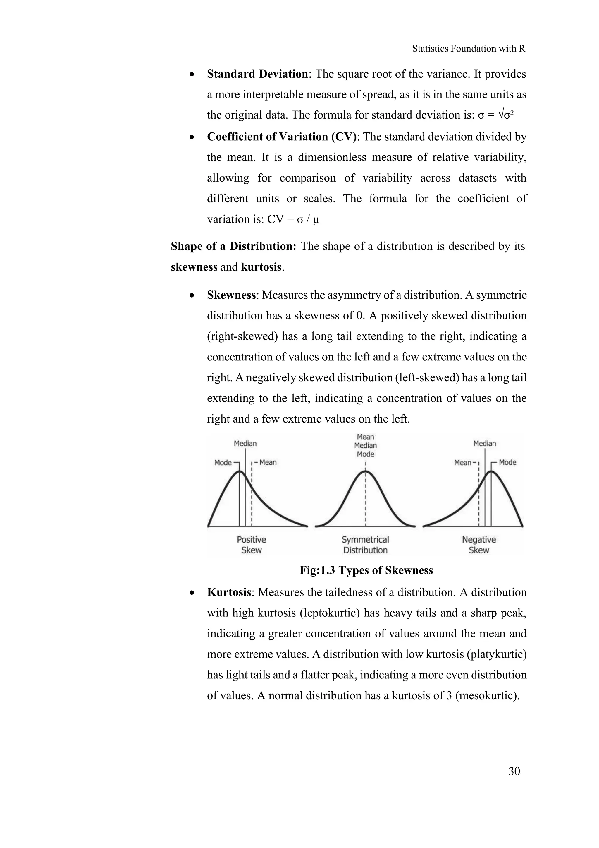
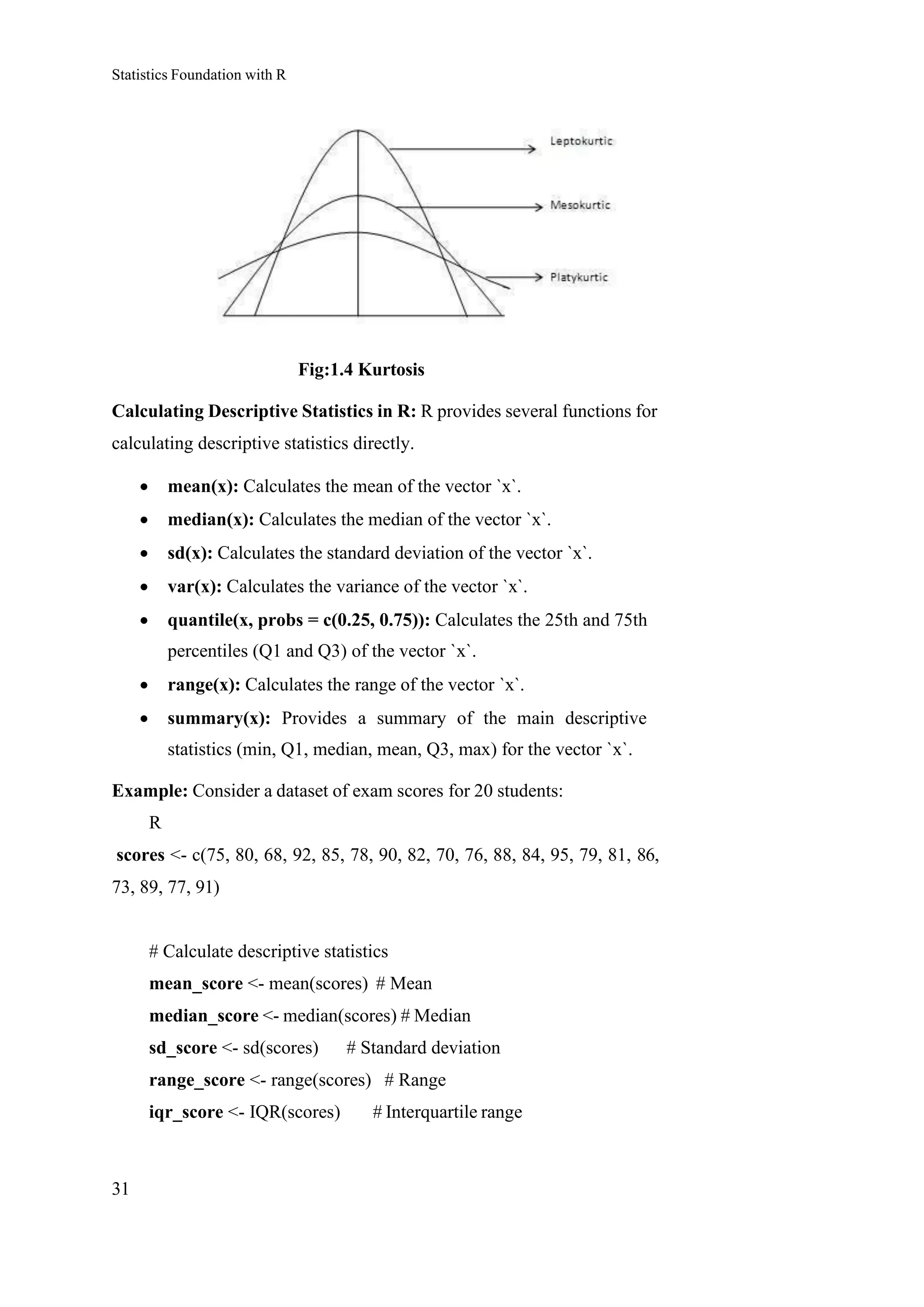
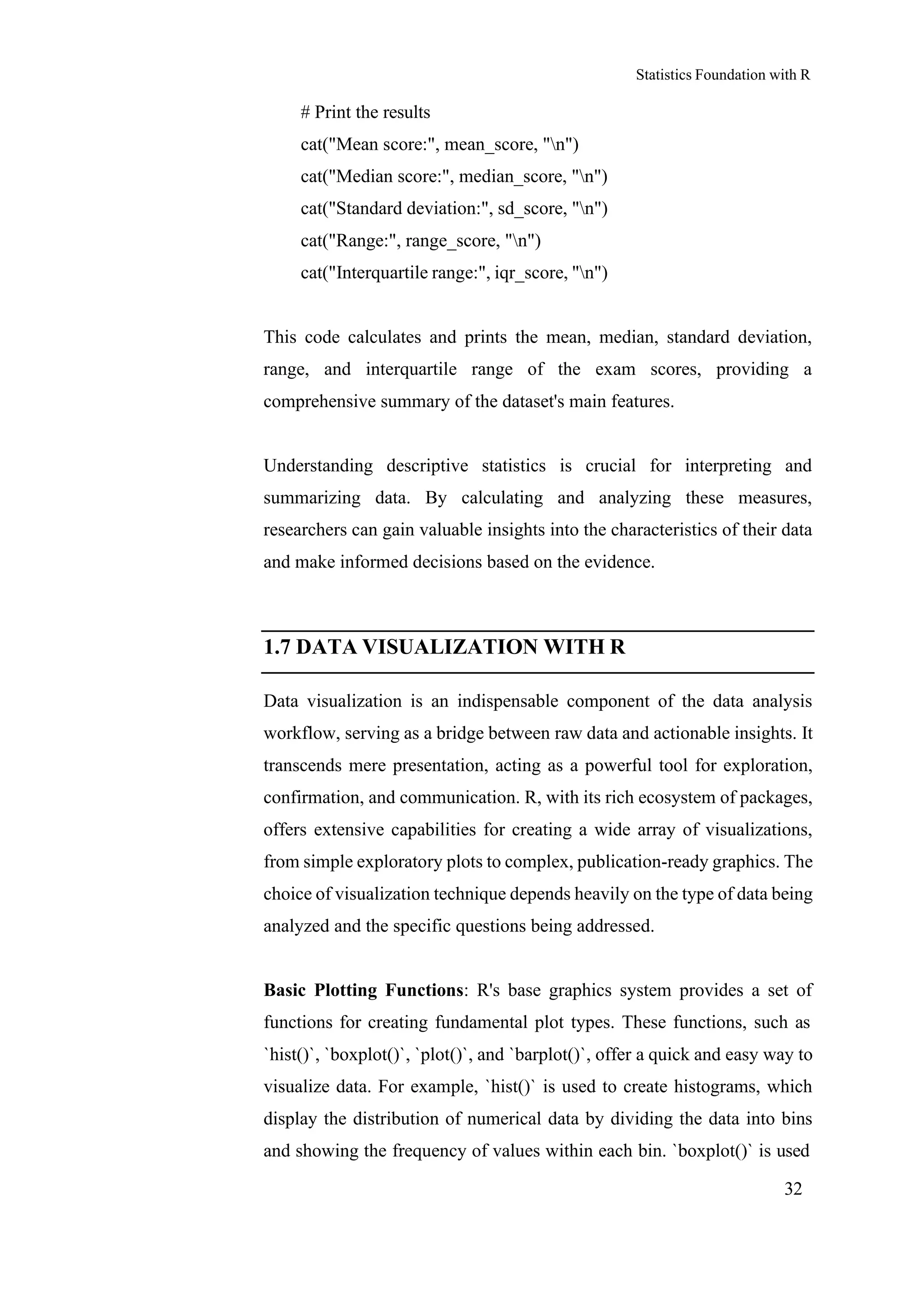
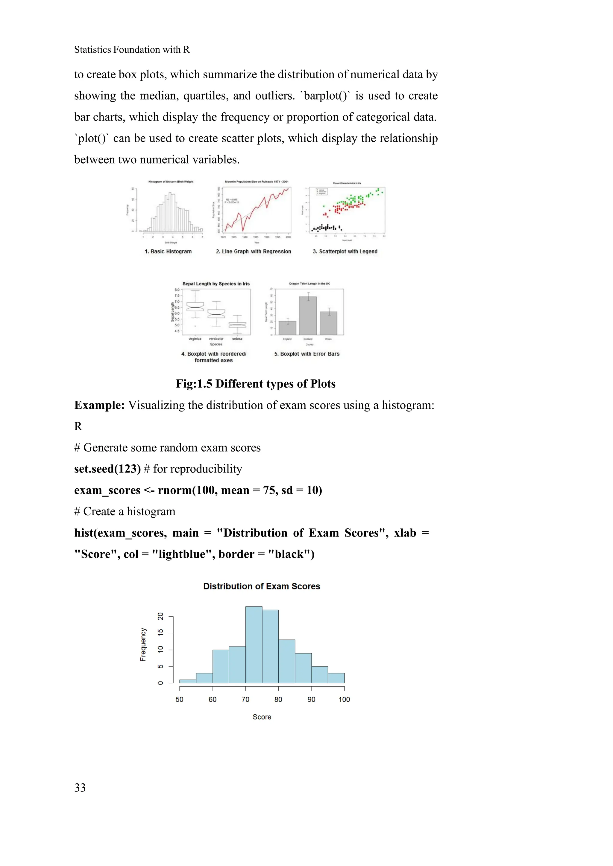

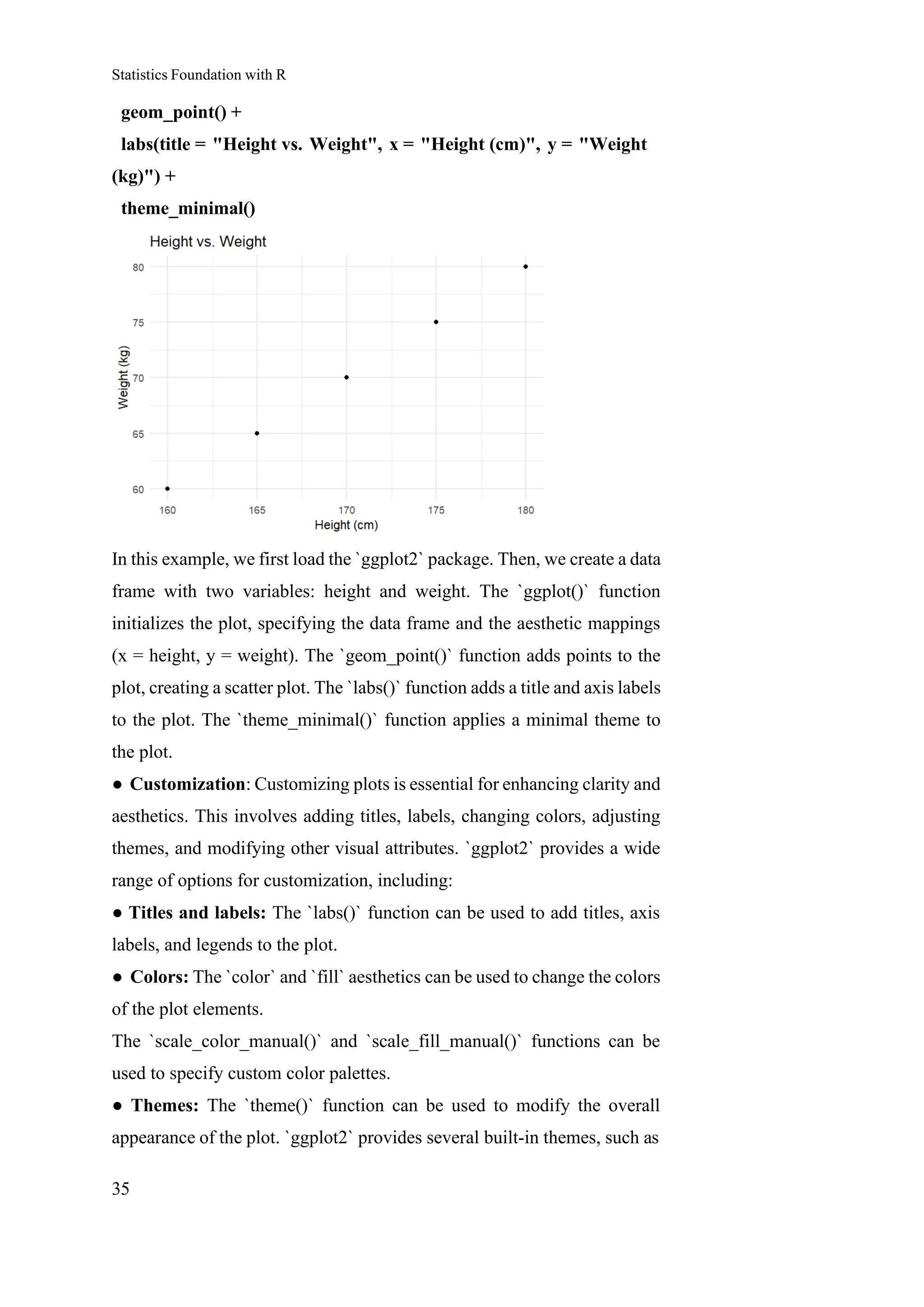


![Statistics Foundation with R
45
Refer 1.4 for Answer to check your progress- 3 Q. 2
Data frames are the most common data structure used in R for data
analysis. They are flexible, allowing columns to have different data types,
which is ideal for storing real-world datasets. Additionally, the availability
of powerful manipulation tools like dplyr makes them essential for data
scientists and statisticians.
Refer 1.4 for Answer to check your progress- 3 Q. 3
The provided content does not contain information about lists in R.
Therefore, I cannot provide a comparison between vectors and lists based
on the given text. The content focuses on vectors, matrices, and data
frames.
Refer 1.5 for Answer to check your progress- 4 Q. 1
In R, missing values are represented as NA, and the `is.na()` function
identifies them. Removal can be done using `na.omit()`, but it may reduce
sample size and introduce bias. Imputation replaces missing values with
estimates like mean imputation using `data$column[is.na(data$column)]
<- mean(data$column, na.rm = TRUE)` or more sophisticated methods
like regression imputation or multiple imputation.
Refer 1.5 for Answer to check your progress- 4 Q. 2
In R, recoding variables can be achieved using functions like ifelse() or
dplyr::case_when() to convert continuous variables into categorical ones
or collapse categories. The dplyr package also offers powerful tools such
as mutate() and recode() for transforming variable values. These methods
allow for flexible and efficient data transformation to suit specific analysis
needs.
Refer 1.5 for Answer to check your progress- 4 Q. 3
To import data from an Excel spreadsheet into R, you can use the
`read_excel()` function from the `readxl` package. This function allows
you to read data from both `.xls` and `.xlsx` files. For example,](https://image.slidesharecdn.com/homibhabha-b-250915190628-bb7fdcda/75/HomiBhabha-B-Sc-Business-AI-Sem-1-Statistics-Foundation-with-R-SLM-pdf-45-2048.jpg)


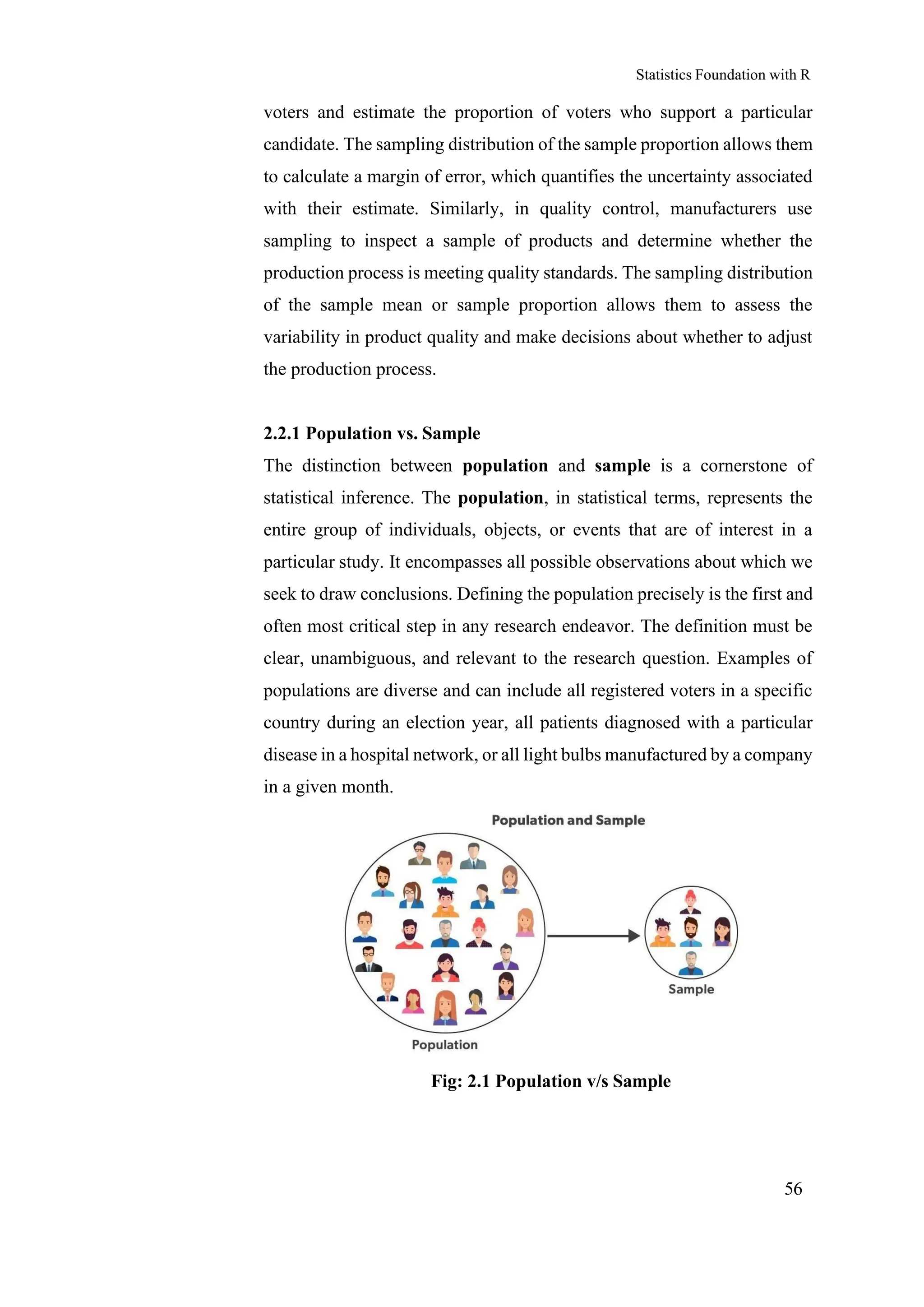

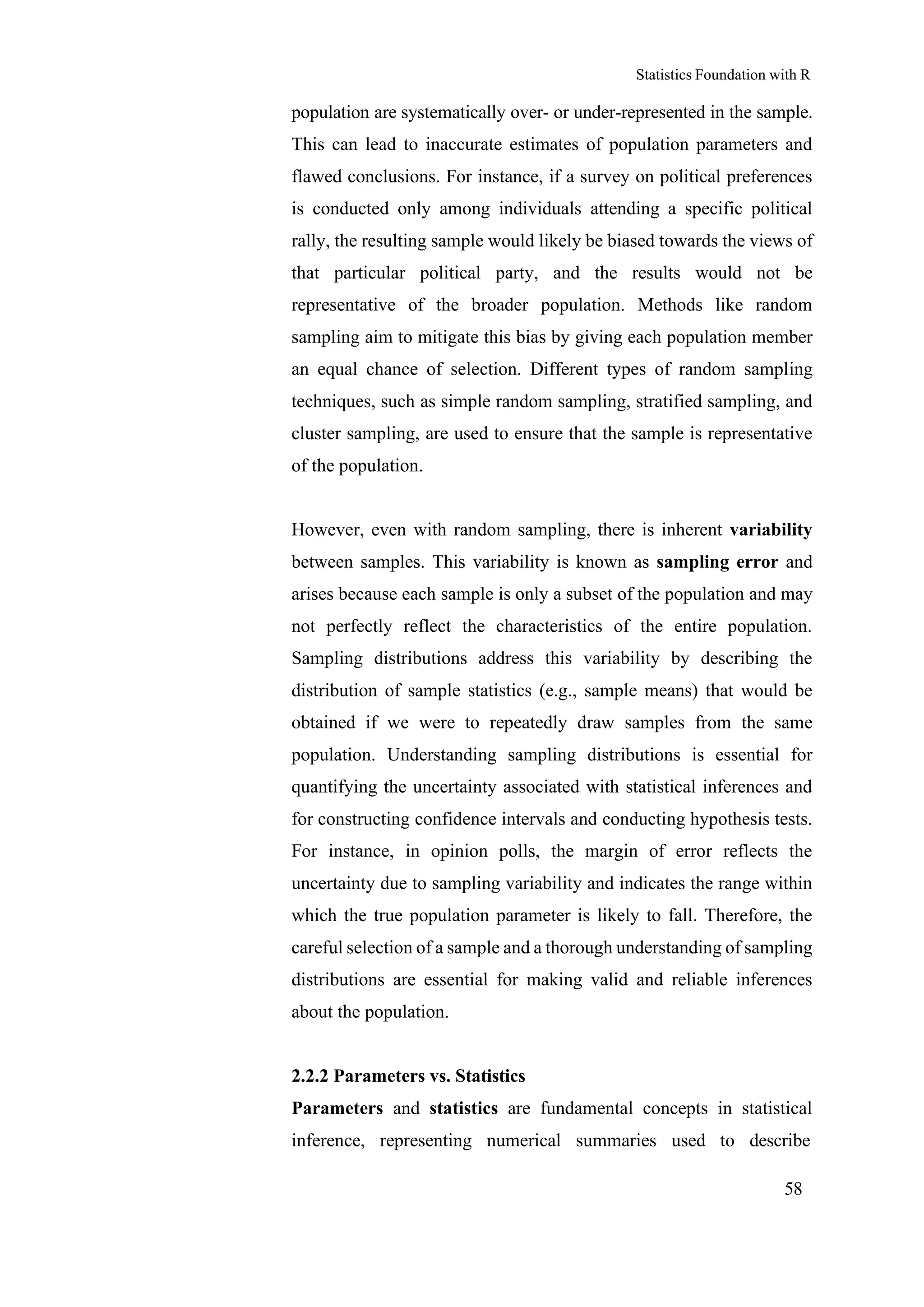


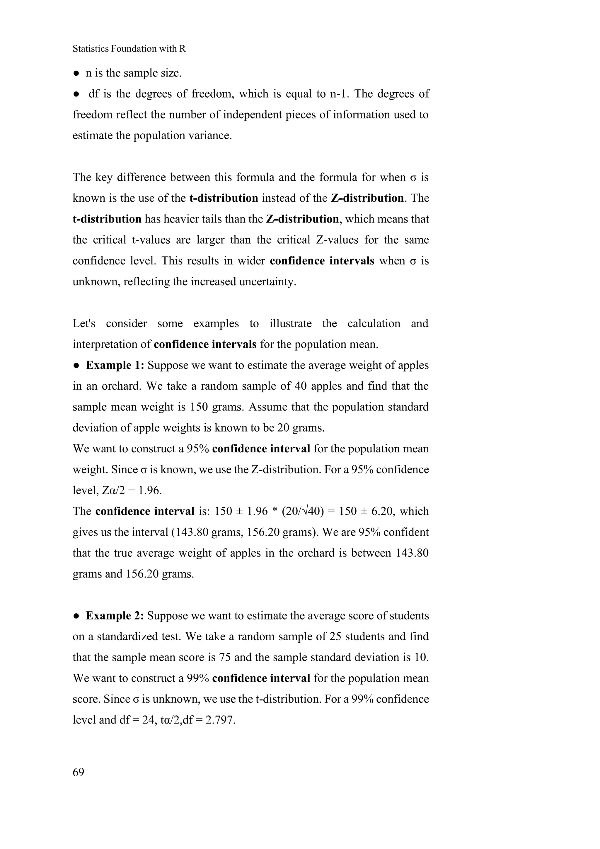


![Statistics Foundation with R
89
which specific groups differ significantly from each other. To determine
which specific groups differ significantly, post-hoc tests are necessary.
Post-hoc tests are pairwise comparisons that control for the familywise
error rate, which is the probability of making at least one Type I error
across all comparisons. Common post-hoc tests include Tukey's HSD test,
Bonferroni correction, Scheffé test, and Dunnett's test. These tests provide
p-values for each pairwise comparison, allowing us to determine which
pairs of groups differ significantly from each other. For example, suppose
we conduct an ANOVA to compare the effectiveness of four different
teaching methods on student test scores. The ANOVA results show a
significant F-statistic and a p-value less than 0.05, indicating that there are
significant differences in test scores among the four teaching methods.
However, the ANOVA does not tell us which specific teaching methods
differ significantly from each other. To determine this, we would perform
post-hoc tests such as Tukey's HSD test. The Tukey's HSD test would
provide p-values for each pairwise comparison of teaching methods,
allowing us to identify which pairs of teaching methods result in
significantly different test scores.
# Create a sample dataset
> # 3 groups: Method A, Method B, Method C
> scores <- c(85, 90, 88, 75, 78, 74, 92, 95, 94)
> method <- factor(c("A", "A", "A", "B", "B", "B", "C", "C", "C"))
>
> # Combine into a data frame
> data <- data.frame(scores, method)
>
> # View the dataset
> print("Dataset:")
[1] "Dataset:"](https://image.slidesharecdn.com/homibhabha-b-250915190628-bb7fdcda/75/HomiBhabha-B-Sc-Business-AI-Sem-1-Statistics-Foundation-with-R-SLM-pdf-89-2048.jpg)
![Statistics Foundation with R
90
# Perform one-way ANOVA
> anova_result <- aov(scores ~ method, data = data)
>
> # Show ANOVA summary (includes F-statistic and p-value)
> print("ANOVA Result:")
[1] "ANOVA Result:"
Check Your Progress -3
1. What is the primary purpose of ANOVA?
.....................................................................................................................
.....................................................................................................................
2. Explain the difference between between-group variance and within-
group variance in ANOVA.
.....................................................................................................................
.....................................................................................................................
3. How is the F-statistic calculated and what does a large F-statistic
indicate?
.....................................................................................................................
.....................................................................................................................](https://image.slidesharecdn.com/homibhabha-b-250915190628-bb7fdcda/75/HomiBhabha-B-Sc-Business-AI-Sem-1-Statistics-Foundation-with-R-SLM-pdf-90-2048.jpg)
![Statistics Foundation with R
92
The test statistic in both types of chi-squared tests is the chi-squared
statistic (χ²), which measures the discrepancy between the observed
frequencies and the expected frequencies. The chi-squared statistic is
calculated as the sum of the squared differences between the observed and
expected frequencies, divided by the expected frequencies.
The formula for the chi-squared statistic is: χ² = Σ [(Oᵢ - Eᵢ)² / Eᵢ] where
Oᵢ represents the observed frequency for category i, and Eᵢ represents the
expected frequency for category i. A large chi-squared statistic indicates a
significant difference between the observed and expected frequencies,
suggesting a relationship between the variables (in the case of the test for
independence) or a deviation from the expected distribution (in the case of
the goodness-of-fit test).
The chi-squared statistic follows a chi-squared distribution, and its
degrees of freedom are determined by the number of categories in the
variable(s) being analyzed. The degrees of freedom for the chi-squared
goodness-of-fit test are equal to the number of categories minus one (k -
1), where k is the number of categories. The degrees of freedom for the
chi-squared test for independence are equal to (r - 1)(c - 1), where r is the
number of rows in the contingency table and c is the number of columns
in the contingency table.](https://image.slidesharecdn.com/homibhabha-b-250915190628-bb7fdcda/75/HomiBhabha-B-Sc-Business-AI-Sem-1-Statistics-Foundation-with-R-SLM-pdf-92-2048.jpg)

![Statistics Foundation with R
94
that the expected frequencies in each cell of the contingency table are
sufficiently large (typically at least 5) to ensure the validity of the chi-
squared test. If the expected frequencies are too small, the chi-squared test
may not be accurate, and alternative tests such as Fisher's exact test may
be more appropriate.
R-Code to perform Chi-Square Test
# Create a contingency table
> # Rows = Gender (Male, Female)
> # Columns = Preference (Like, Dislike)
>
> data <- matrix(c(30, 10, 20, 40), # Counts
+ nrow = 2, # 2 genders
+ byrow = TRUE)
>
> # Add row and column names for clarity
> rownames(data) <- c("Male", "Female")
> colnames(data) <- c("Like", "Dislike")
>
> # Print the data table
> print("Contingency Table:")
[1] "Contingency Table:"
> print(data)
> # Perform Chi-Square Test of Independence
> chi_result <- chisq.test(data)
>
> # Print test results
> print("Chi-Square Test Result:")
[1] "Chi-Square Test Result:"](https://image.slidesharecdn.com/homibhabha-b-250915190628-bb7fdcda/75/HomiBhabha-B-Sc-Business-AI-Sem-1-Statistics-Foundation-with-R-SLM-pdf-94-2048.jpg)


![Statistics Foundation with R
100
familywise error rate, which is the probability of making at least one
Type I error across all comparisons. Common post-hoc tests include
Tukey's HSD test, Bonferroni correction, Scheffé test, and Dunnett's
test, which provide p-values for each pairwise comparison, allowing us to
determine which pairs of groups differ significantly from each other.
Refer 2.8 for Answer to check your progress- 4 Q. 1
Chi-squared tests are used to analyze categorical data. Categorical data
consists of variables divided into distinct categories or groups. These tests
examine the relationships between categorical variables, determining if
observed frequencies differ from expected frequencies or if variables are
independent.
Refer 2.8 for Answer to check your progress- 4 Q. 2
The chi-squared goodness-of-fit test assesses if the observed frequencies
of categories in a single categorical variable differ significantly from
expected frequencies, based on a theoretical distribution. In contrast, the
chi-squared test for independence examines the association between two
categorical variables to determine if they are independent of each other,
using a contingency table to compare observed and expected frequencies.
Refer 2.8 for Answer to check your progress- 4 Q. 3
The chi-squared statistic (χ²) is calculated as the sum of the squared
differences between the observed and expected frequencies, divided by the
expected frequencies, using the formula: χ² = Σ [(Oᵢ - Eᵢ)² / Eᵢ]. Here, Oᵢ
represents the observed frequency for category i, and Eᵢ represents the
expected frequency for category i. A large chi-squared statistic indicates
a significant difference between the observed and expected frequencies,
suggesting a relationship between the variables (in the case of the test for
independence) or a deviation from the expected distribution (in the case
of the goodness-of-fit test).](https://image.slidesharecdn.com/homibhabha-b-250915190628-bb7fdcda/75/HomiBhabha-B-Sc-Business-AI-Sem-1-Statistics-Foundation-with-R-SLM-pdf-100-2048.jpg)


![Statistics Foundation with R
111
other. The coefficient ranges from -1 to +1, providing a clear indication of
both the direction and strength of the linear relationship. A positive
coefficient indicates a direct relationship, where both variables increase or
decrease together, while a negative coefficient indicates an inverse
relationship, where one variable increases as the other decreases. A
coefficient of 0 suggests no linear relationship between the variables.
Fig: 3.1 Types of Correlation
The mathematical formula for calculating Pearson's correlation coefficient
is as follows:
r = Σ[(xi - x
̄ )(yi - ȳ)] / [√(Σ(xi - x
̄ )²) * √(Σ(yi - ȳ)²)]
where:
● xi and yi are the individual data points for variables x and y
● x
̄ and ȳ are the means of variables x and y
● Σ denotes the summation operator
This formula calculates the covariance between the two variables,
normalized by the product of their standard deviations. This normalization
ensures that the correlation coefficient is scale-invariant, meaning that it is
not affected by changes in the units of measurement of the variables.
Consider the following examples to illustrate the interpretation of
Pearson's correlation coefficient:
● Example 1: A researcher investigates the relationship between hours
studied and exam scores for a group of students. The calculated Pearson's](https://image.slidesharecdn.com/homibhabha-b-250915190628-bb7fdcda/75/HomiBhabha-B-Sc-Business-AI-Sem-1-Statistics-Foundation-with-R-SLM-pdf-111-2048.jpg)
![Statistics Foundation with R
114
The key difference between Spearman's rho and Pearson's correlation
coefficient lies in the data they utilize. Pearson's correlation works directly
with the raw values of the variables, while Spearman's rho operates on the
ranks of those values. This transformation to ranks makes Spearman's rho
less sensitive to outliers and suitable for ordinal data, where the values
represent ordered categories rather than precise measurements.
The calculation of Spearman's rho involves the following steps:
1. Rank the data: Assign ranks to the values of each variable separately.
If there are ties (i.e., two or more values are the same), assign the average
rank to those values.
2. Calculate the differences: For each pair of data points, calculate the
difference (d) between the ranks of the two variables.
3. Square the differences: Square each of the differences calculated in
the previous step.
4. Sum the squared differences: Add up all the squared differences.
5. Apply the formula: Calculate Spearman's rho using the following
formula:
ρ = 1 - [6 * Σ(d²)] / [n * (n² - 1)]
where:
● ρ is Spearman's rank correlation coefficient
● Σ(d²) is the sum of the squared differences between ranks
● n is the number of data points
Consider the following examples to illustrate the application and
interpretation of Spearman's rho:
● Example 1: A teacher wants to assess the relationship between students'
rankings in a math test and their rankings in a science test. Spearman's rho
is calculated to be 0.75. This indicates a strong positive monotonic
relationship, suggesting that students who rank highly in math tend to also
rank highly in science.](https://image.slidesharecdn.com/homibhabha-b-250915190628-bb7fdcda/75/HomiBhabha-B-Sc-Business-AI-Sem-1-Statistics-Foundation-with-R-SLM-pdf-114-2048.jpg)


![Statistics Foundation with R
117
The least squares method is the most common technique for estimating
the values of β0 and β1. This method aims to minimize the sum of the
squared differences between the observed Y values and the values
predicted by the model. In other words, it finds the line that best fits the
data by minimizing the overall prediction error. The formulas for
calculating β0 and β1 are derived from calculus and linear algebra,
ensuring the best possible fit under the least squares criterion. Specifically:
β1 = Σ[(Xi - X
̄ )(Yi - Ȳ)] / Σ[(Xi - X
̄ )²],
where X
̄ and Ȳ are the means of X and Y, respectively.
β0 = Ȳ - β1X
̄
The interpretation of the coefficients is crucial for understanding the
relationship between X and Y.
The slope (β1) indicates the magnitude and direction of the effect of X on
Y. A positive slope means that as X increases, Y tends to increase, while
a negative slope indicates that as X increases, Y tends to decrease.
The intercept (β0), while mathematically defined, may not always have a
practical interpretation, especially if X cannot realistically take on a value
of zero. For example, in a model predicting crop yield based on fertilizer
amount, the intercept would represent the predicted yield with no fertilizer,
which might be a theoretical rather than practical value.
Assessing the goodness of fit of the model is essential to determine how
well the regression line represents the data. R-squared (R²) is a commonly
used metric for this purpose. R-squared represents the proportion of the
variance in Y that is explained by X. It ranges from 0 to 1, with higher
values indicating a better fit. For instance, an R-squared of 0.80 means that
80% of the variability in Y is explained by the linear relationship with X.
However, R-squared should be interpreted with caution, as it can be
inflated by adding more predictor variables to the model, even if those
variables are not truly related to Y. Adjusted R-squared addresses this
issue by penalizing the inclusion of unnecessary predictors.](https://image.slidesharecdn.com/homibhabha-b-250915190628-bb7fdcda/75/HomiBhabha-B-Sc-Business-AI-Sem-1-Statistics-Foundation-with-R-SLM-pdf-117-2048.jpg)


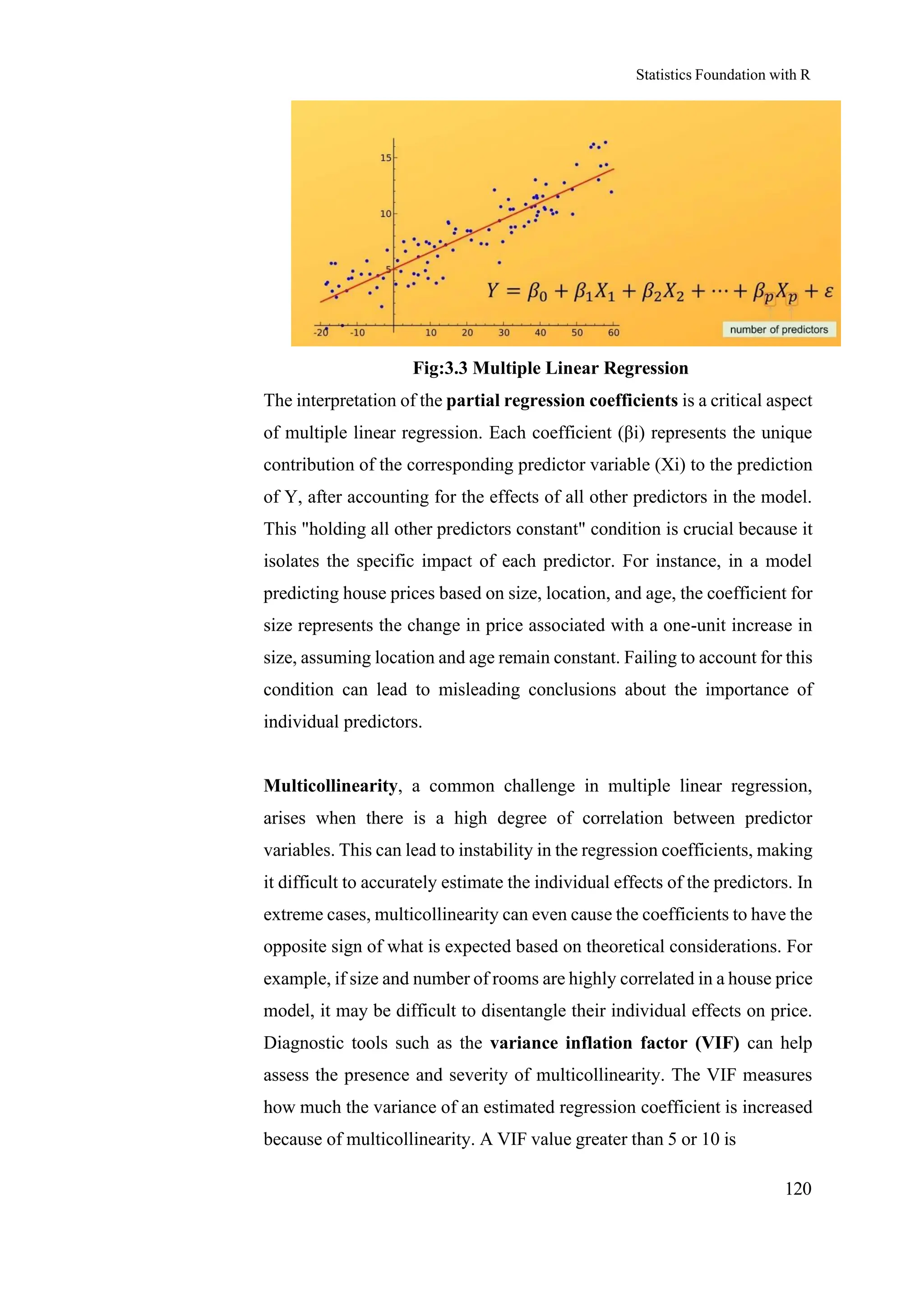


![Basics of R programming for analytics [Autosaved] (1).pdf](https://cdn.slidesharecdn.com/ss_thumbnails/basicsofrprogrammingforanalyticsautosaved1-240916080545-0682f8c8-thumbnail.jpg?width=640&height=640&fit=bounds)