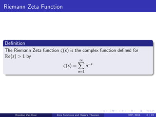
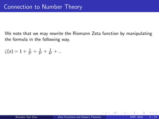
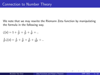
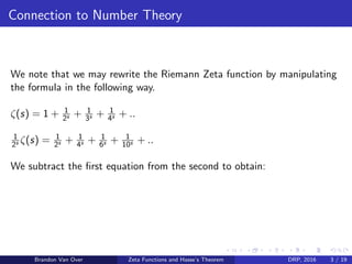
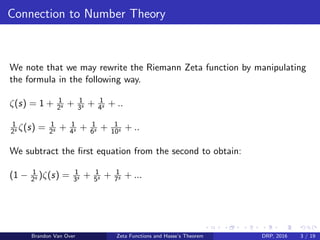
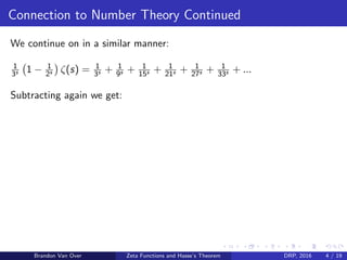
The document discusses zeta functions and their connection to number theory and algebraic geometry. It defines the Riemann zeta function and shows how it can be rewritten as an infinite product over prime numbers. This generalization is extended to Dedekind domains and used to define zeta functions for curves over finite fields. Properties of these curve zeta functions are explored, including a formula relating their coefficients to the number of points on the curves over finite fields.

1. Zeta Functions and Hasse’s Theorem
Brandon Van Over
DRP, 2016
Brandon Van Over Zeta Functions and Hasse’s Theorem DRP, 2016 1 / 19

2. Riemann Zeta Function
Definition
The Riemann Zeta function ζ(s) is the complex function defined for
Re(s) > 1 by
ζ(s) =
∞
n=1
n−s
Brandon Van Over Zeta Functions and Hasse’s Theorem DRP, 2016 2 / 19

3. Connection to Number Theory
We note that we may rewrite the Riemann Zeta function by manipulating
the formula in the following way.
Brandon Van Over Zeta Functions and Hasse’s Theorem DRP, 2016 3 / 19

4. Connection to Number Theory
We note that we may rewrite the Riemann Zeta function by manipulating
the formula in the following way.
ζ(s) = 1 + 1
2s + 1
3s + 1
4s + ..
Brandon Van Over Zeta Functions and Hasse’s Theorem DRP, 2016 3 / 19

5. Connection to Number Theory
We note that we may rewrite the Riemann Zeta function by manipulating
the formula in the following way.
ζ(s) = 1 + 1
2s + 1
3s + 1
4s + ..
1
2s ζ(s) = 1
2s + 1
4s + 1
6s + 1
10s + ..
Brandon Van Over Zeta Functions and Hasse’s Theorem DRP, 2016 3 / 19

6. Connection to Number Theory
We note that we may rewrite the Riemann Zeta function by manipulating
the formula in the following way.
ζ(s) = 1 + 1
2s + 1
3s + 1
4s + ..
1
2s ζ(s) = 1
2s + 1
4s + 1
6s + 1
10s + ..
We subtract the first equation from the second to obtain:
Brandon Van Over Zeta Functions and Hasse’s Theorem DRP, 2016 3 / 19

7. Connection to Number Theory
We note that we may rewrite the Riemann Zeta function by manipulating
the formula in the following way.
ζ(s) = 1 + 1
2s + 1
3s + 1
4s + ..
1
2s ζ(s) = 1
2s + 1
4s + 1
6s + 1
10s + ..
We subtract the first equation from the second to obtain:
(1 − 1
2s )ζ(s) = 1
3s + 1
5s + 1
7s + ...
Brandon Van Over Zeta Functions and Hasse’s Theorem DRP, 2016 3 / 19

8. Connection to Number Theory Continued
We continue on in a similar manner:
1
3s 1 − 1
2s ζ(s) = 1
3s + 1
9s + 1
15s + 1
21s + 1
27s + 1
33s + ...
Subtracting again we get:
Brandon Van Over Zeta Functions and Hasse’s Theorem DRP, 2016 4 / 19

9. Connection to Number Theory Continued
We continue on in a similar manner:
1
3s 1 − 1
2s ζ(s) = 1
3s + 1
9s + 1
15s + 1
21s + 1
27s + 1
33s + ...
Subtracting again we get:
1 − 1
3s 1 − 1
2s ζ(s) = 1 + 1
5s + 1
7s + 1
11s + 1
13s + 1
17s + . . .
Brandon Van Over Zeta Functions and Hasse’s Theorem DRP, 2016 4 / 19

10. Connection to Number Theory Continued
We continue on in a similar manner:
1
3s 1 − 1
2s ζ(s) = 1
3s + 1
9s + 1
15s + 1
21s + 1
27s + 1
33s + ...
Subtracting again we get:
1 − 1
3s 1 − 1
2s ζ(s) = 1 + 1
5s + 1
7s + 1
11s + 1
13s + 1
17s + . . .
We can see that we have gotten rid of all denominators which are
multiples of 2 and 3.
Brandon Van Over Zeta Functions and Hasse’s Theorem DRP, 2016 4 / 19

11. Connection to Number Theory Continued
We continue on in a similar manner:
1
3s 1 − 1
2s ζ(s) = 1
3s + 1
9s + 1
15s + 1
21s + 1
27s + 1
33s + ...
Subtracting again we get:
1 − 1
3s 1 − 1
2s ζ(s) = 1 + 1
5s + 1
7s + 1
11s + 1
13s + 1
17s + . . .
We can see that we have gotten rid of all denominators which are
multiples of 2 and 3.
We note that if we repeat this process infinitely many times, we obtain:
Brandon Van Over Zeta Functions and Hasse’s Theorem DRP, 2016 4 / 19

12. Connection to Number Theory Continued
We continue on in a similar manner:
1
3s 1 − 1
2s ζ(s) = 1
3s + 1
9s + 1
15s + 1
21s + 1
27s + 1
33s + ...
Subtracting again we get:
1 − 1
3s 1 − 1
2s ζ(s) = 1 + 1
5s + 1
7s + 1
11s + 1
13s + 1
17s + . . .
We can see that we have gotten rid of all denominators which are
multiples of 2 and 3.
We note that if we repeat this process infinitely many times, we obtain:
. . . 1 − 1
11s 1 − 1
7s 1 − 1
5s 1 − 1
3s 1 − 1
2s ζ(s) = 1
Brandon Van Over Zeta Functions and Hasse’s Theorem DRP, 2016 4 / 19

13. The Result
Dividing both side by our product we obtain:
Brandon Van Over Zeta Functions and Hasse’s Theorem DRP, 2016 5 / 19

14. The Result
Dividing both side by our product we obtain:
ζ(s) =
1
1 − 1
2s 1 − 1
3s 1 − 1
5s 1 − 1
7s 1 − 1
11s . . .
=
p prime
1
1 − p−s
Brandon Van Over Zeta Functions and Hasse’s Theorem DRP, 2016 5 / 19

15. The Famous Conjecture
All of the zeroes of ζ(s) where 0 ≤ Re(s) ≤ 1 lie on the line
Re(s) = 1
2.
Brandon Van Over Zeta Functions and Hasse’s Theorem DRP, 2016 6 / 19

16. Dedekind’s Generalization to More General Rings
Later on Riemann’s theory was generalized to an arbitrary Dedekind
domain A with finite quotients in the following manner:
Brandon Van Over Zeta Functions and Hasse’s Theorem DRP, 2016 7 / 19

17. Dedekind’s Generalization to More General Rings
Later on Riemann’s theory was generalized to an arbitrary Dedekind
domain A with finite quotients in the following manner:
ζA(s) =
a
(Na)−s
Brandon Van Over Zeta Functions and Hasse’s Theorem DRP, 2016 7 / 19

18. Dedekind’s Generalization to More General Rings
Later on Riemann’s theory was generalized to an arbitrary Dedekind
domain A with finite quotients in the following manner:
ζA(s) =
a
(Na)−s
ζA(s) =
p
(1 − (Np)−s
)−1
Where a an ideal of A, and Na is the number of cosets in A/a.
Brandon Van Over Zeta Functions and Hasse’s Theorem DRP, 2016 7 / 19

19. Dedekind’s Generalization to More General Rings
Later on Riemann’s theory was generalized to an arbitrary Dedekind
domain A with finite quotients in the following manner:
ζA(s) =
a
(Na)−s
ζA(s) =
p
(1 − (Np)−s
)−1
Where a an ideal of A, and Na is the number of cosets in A/a.
Note: ζZ(s) is Riemann’s function.
Brandon Van Over Zeta Functions and Hasse’s Theorem DRP, 2016 7 / 19

20. Here Comes Algebraic Geometry
We begin with an absolutely irreducible polynomial f ∈ Fq[x, y] such that
Zf ( ¯Fq) is nonsingular. Denote the associated coordinate ring Fq[x, y]/(f )
by Cf .
Brandon Van Over Zeta Functions and Hasse’s Theorem DRP, 2016 8 / 19

21. Here Comes Algebraic Geometry
We begin with an absolutely irreducible polynomial f ∈ Fq[x, y] such that
Zf ( ¯Fq) is nonsingular. Denote the associated coordinate ring Fq[x, y]/(f )
by Cf .
It can be shown that the coordinate ring is a Dedekind domain with finite
quotients, and so we may apply what we previously discussed to obtain a
zeta function associated to this curve:
ζ(Cf , s) =
M∈Max(Cf )
(1 − (N(M))−s
)−1
.
Brandon Van Over Zeta Functions and Hasse’s Theorem DRP, 2016 8 / 19

22. Here Comes Algebraic Geometry
We begin with an absolutely irreducible polynomial f ∈ Fq[x, y] such that
Zf ( ¯Fq) is nonsingular. Denote the associated coordinate ring Fq[x, y]/(f )
by Cf .
It can be shown that the coordinate ring is a Dedekind domain with finite
quotients, and so we may apply what we previously discussed to obtain a
zeta function associated to this curve:
ζ(Cf , s) =
M∈Max(Cf )
(1 − (N(M))−s
)−1
.
Note: In a Dedekind ring all prime ideals are maximal, which explains the
change of indexing in the product.
Brandon Van Over Zeta Functions and Hasse’s Theorem DRP, 2016 8 / 19

23. But First, A Nice Fact
Theorem
Let q = pn, and let ¯Fq be the algebraic closure of Fq. Let Fqn be the
unique subfield of ¯Fq of degree n over Fq. Let f ∈ Fq be absolutely
irreducible, and Cf its coordinate ring. Then the sets
{M ∈ Max(Cf ) : [Cf /M : Fq] = d} and Zf (Fqn ) are finite. Let
Nn = |Zf (Fqn )| and bd = |{M ∈ Max(Cf ) : [Cf /M : Fq] = d}|. Then
Nn = d|n dbd .
Brandon Van Over Zeta Functions and Hasse’s Theorem DRP, 2016 9 / 19

24. Back To Zeta Functions
Knowing that bd is finite, and noting that Cf /M ∼= Fqd for
M ∈ {M ∈ Max(Cf ) : [Cf /M : Fq] = d} we may group our product in the
following manner:
Brandon Van Over Zeta Functions and Hasse’s Theorem DRP, 2016 10 / 19

25. Back To Zeta Functions
Knowing that bd is finite, and noting that Cf /M ∼= Fqd for
M ∈ {M ∈ Max(Cf ) : [Cf /M : Fq] = d} we may group our product in the
following manner:
d∈N
(1 − (N(M)−s
))−bd
=
d∈N
(1 −
1
qds
))−bd
Brandon Van Over Zeta Functions and Hasse’s Theorem DRP, 2016 10 / 19

26. Back To Zeta Functions
Knowing that bd is finite, and noting that Cf /M ∼= Fqd for
M ∈ {M ∈ Max(Cf ) : [Cf /M : Fq] = d} we may group our product in the
following manner:
d∈N
(1 − (N(M)−s
))−bd
=
d∈N
(1 −
1
qds
))−bd
Allowing 1
qs = T, we obtain that:
Brandon Van Over Zeta Functions and Hasse’s Theorem DRP, 2016 10 / 19

27. Back To Zeta Functions
Knowing that bd is finite, and noting that Cf /M ∼= Fqd for
M ∈ {M ∈ Max(Cf ) : [Cf /M : Fq] = d} we may group our product in the
following manner:
d∈N
(1 − (N(M)−s
))−bd
=
d∈N
(1 −
1
qds
))−bd
Allowing 1
qs = T, we obtain that:
ζ(Cf , T) = d∈N(1 − Td )−bd
Brandon Van Over Zeta Functions and Hasse’s Theorem DRP, 2016 10 / 19

28. Back To Zeta Functions
Knowing that bd is finite, and noting that Cf /M ∼= Fqd for
M ∈ {M ∈ Max(Cf ) : [Cf /M : Fq] = d} we may group our product in the
following manner:
d∈N
(1 − (N(M)−s
))−bd
=
d∈N
(1 −
1
qds
))−bd
Allowing 1
qs = T, we obtain that:
ζ(Cf , T) = d∈N(1 − Td )−bd
After taking the log of both sides, using the power series expansion of log,
rearranging sums, and exponentiating we arrive at a nice formula for....
Brandon Van Over Zeta Functions and Hasse’s Theorem DRP, 2016 10 / 19

29. Definition
Let f ∈ Fq[x, y] be an absolutely irreducible polynomial, and assume that
Zf is nonsingular. Then the power series
Z(Zf /Fq, T) := Z(Cf , T) = exp( ∞
n=1 Nn
Tn
n ) is called the zeta function
of the affine curve Zf /Fq.
Brandon Van Over Zeta Functions and Hasse’s Theorem DRP, 2016 11 / 19

30. Definition
Let f ∈ Fq[x, y] be an absolutely irreducible polynomial, and assume that
Zf is nonsingular. Then the power series
Z(Zf /Fq, T) := Z(Cf , T) = exp( ∞
n=1 Nn
Tn
n ) is called the zeta function
of the affine curve Zf /Fq.
Example
The Affine line A1(Fqn ) consists of qn points, and so we have that
Z(A1/Fq, T) = exp( ∞
n=1 qn Tn
n ) = exp(− log(1 − qT)) = (1 − qT)−1.
Brandon Van Over Zeta Functions and Hasse’s Theorem DRP, 2016 11 / 19

31. Basics of Projective Space
We start with an n + 1 dimensional vector space over a field k with basis
{e0, ..., en}, and define the map
n
i=0
ci ei → (c0, ..., cn) ∈ kn+1
.
Brandon Van Over Zeta Functions and Hasse’s Theorem DRP, 2016 12 / 19

32. Basics of Projective Space
We start with an n + 1 dimensional vector space over a field k with basis
{e0, ..., en}, and define the map
n
i=0
ci ei → (c0, ..., cn) ∈ kn+1
.
We then consider kn+1 {(0, ..., 0)} modulo the action of k∗ on kn+1
defined as λ(c0, ..., cn) := (λc0, ..., λcn). Thus our system of coordinates
consists of the orbits of the action of k∗.
Brandon Van Over Zeta Functions and Hasse’s Theorem DRP, 2016 12 / 19

33. Basics of Projective Space
We start with an n + 1 dimensional vector space over a field k with basis
{e0, ..., en}, and define the map
n
i=0
ci ei → (c0, ..., cn) ∈ kn+1
.
We then consider kn+1 {(0, ..., 0)} modulo the action of k∗ on kn+1
defined as λ(c0, ..., cn) := (λc0, ..., λcn). Thus our system of coordinates
consists of the orbits of the action of k∗.
In less fancy terms, we consider (c0, ..., cn) = (b0, ..., bn) if one is a scalar
multiple of the other, and we denote this equivalence class of points by
(c0 : · · · : cn), and the set of these is denoted Pn(k).
Brandon Van Over Zeta Functions and Hasse’s Theorem DRP, 2016 12 / 19

34. To be able to study curves in projective space, we need to ensure that the
whole equivalence class of a zero is still a zero of the polynomial in
question.
To remedy this we consider homogeneous polynomials, as we then have
that F(λc0, ..., λcn) = λF(c0, .., cn).
Brandon Van Over Zeta Functions and Hasse’s Theorem DRP, 2016 13 / 19

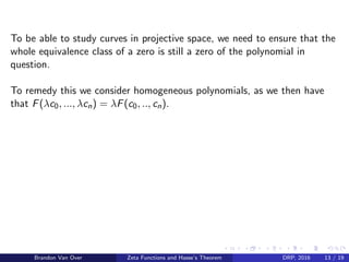
35. To be able to study curves in projective space, we need to ensure that the
whole equivalence class of a zero is still a zero of the polynomial in
question.
To remedy this we consider homogeneous polynomials, as we then have
that F(λc0, ..., λcn) = λF(c0, .., cn).
Definition
A plane projective curve is the set
XF (k) := {(c0 : c1 : c2) ∈ P2(k) : F(a0, a1, a2) = 0} for some
F ∈ k[x0, x1, x2].
Brandon Van Over Zeta Functions and Hasse’s Theorem DRP, 2016 13 / 19

36. To be able to study curves in projective space, we need to ensure that the
whole equivalence class of a zero is still a zero of the polynomial in
question.
To remedy this we consider homogeneous polynomials, as we then have
that F(λc0, ..., λcn) = λF(c0, .., cn).
Definition
A plane projective curve is the set
XF (k) := {(c0 : c1 : c2) ∈ P2(k) : F(a0, a1, a2) = 0} for some
F ∈ k[x0, x1, x2].
Note:The same formula for the zeta function of affine curves holds for
projective curves.
Brandon Van Over Zeta Functions and Hasse’s Theorem DRP, 2016 13 / 19

37. What’s So Great About Projective Plane Curves?
Brandon Van Over Zeta Functions and Hasse’s Theorem DRP, 2016 14 / 19

38. What’s So Great About Projective Plane Curves?
Their zeta functions can be expressed as rational functions with
coefficients in Z, namely for a homogeneous polynomial F of degree d:
Brandon Van Over Zeta Functions and Hasse’s Theorem DRP, 2016 14 / 19

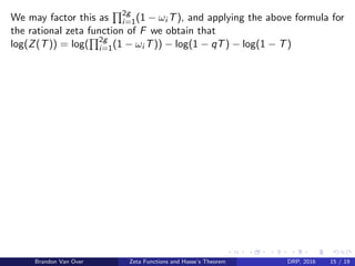
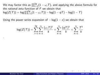
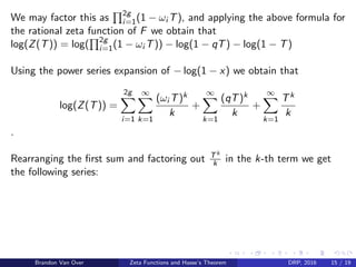
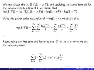
39. What’s So Great About Projective Plane Curves?
Their zeta functions can be expressed as rational functions with
coefficients in Z, namely for a homogeneous polynomial F of degree d:
Z(XF /Fq, T) =
f (T)
(1 − qT)(1 − T)
Where f (T) ∈ Z[X] is a polynomial of degree
2g = 2(d−1)(d−2)
2 = (d − 1)(d − 2).
We have f (0) = 1 by the exponentiation formula, and so we have that
f (T) = 1 + 2g
i=1 ci Ti .
Brandon Van Over Zeta Functions and Hasse’s Theorem DRP, 2016 14 / 19

40. We may factor this as 2g
i=1(1 − ωi T), and applying the above formula for
the rational zeta function of F we obtain that
log(Z(T)) = log( 2g
i=1(1 − ωi T)) − log(1 − qT) − log(1 − T)
Brandon Van Over Zeta Functions and Hasse’s Theorem DRP, 2016 15 / 19

41. We may factor this as 2g
i=1(1 − ωi T), and applying the above formula for
the rational zeta function of F we obtain that
log(Z(T)) = log( 2g
i=1(1 − ωi T)) − log(1 − qT) − log(1 − T)
Using the power series expansion of − log(1 − x) we obtain that
log(Z(T)) =
2g
i=1
∞
k=1
(ωi T)k
k
+
∞
k=1
(qT)k
k
+
∞
k=1
Tk
k
.
Brandon Van Over Zeta Functions and Hasse’s Theorem DRP, 2016 15 / 19

42. We may factor this as 2g
i=1(1 − ωi T), and applying the above formula for
the rational zeta function of F we obtain that
log(Z(T)) = log( 2g
i=1(1 − ωi T)) − log(1 − qT) − log(1 − T)
Using the power series expansion of − log(1 − x) we obtain that
log(Z(T)) =
2g
i=1
∞
k=1
(ωi T)k
k
+
∞
k=1
(qT)k
k
+
∞
k=1
Tk
k
.
Rearranging the first sum and factoring out Tk
k in the k-th term we get
the following series:
Brandon Van Over Zeta Functions and Hasse’s Theorem DRP, 2016 15 / 19

43. We may factor this as 2g
i=1(1 − ωi T), and applying the above formula for
the rational zeta function of F we obtain that
log(Z(T)) = log( 2g
i=1(1 − ωi T)) − log(1 − qT) − log(1 − T)
Using the power series expansion of − log(1 − x) we obtain that
log(Z(T)) =
2g
i=1
∞
k=1
(ωi T)k
k
+
∞
k=1
(qT)k
k
+
∞
k=1
Tk
k
.
Rearranging the first sum and factoring out Tk
k in the k-th term we get
the following series:
∞
k=1
(−
2g
i=1
ωk
i + qk
+ 1)
Tk
k
Brandon Van Over Zeta Functions and Hasse’s Theorem DRP, 2016 15 / 19

44. Number of Solutions
Recall Nk = |XF (Fqk )|, and that Z(XF /Fq, T) = exp( ∞
n=1 Nn
Tn
n )
Brandon Van Over Zeta Functions and Hasse’s Theorem DRP, 2016 16 / 19

45. Number of Solutions
Recall Nk = |XF (Fqk )|, and that Z(XF /Fq, T) = exp( ∞
n=1 Nn
Tn
n )
Equating power series gives us that Nk = − 2g
i=1 ωk
i + qk + 1.
Brandon Van Over Zeta Functions and Hasse’s Theorem DRP, 2016 16 / 19

46. Riemann Hypothesis for Curves
We can write our zeta function of our curve as a function of s by writing
T = q−s.
Brandon Van Over Zeta Functions and Hasse’s Theorem DRP, 2016 17 / 19

47. Riemann Hypothesis for Curves
We can write our zeta function of our curve as a function of s by writing
T = q−s.
The Riemann hypothesis for curves over finite fields states that if
0 ≤ Re(s) ≤ 1, and Z(XF /Fq, q−s) = 0 then Re(s) = 1
2. Since our
solutions look like 1
ωi
= q−s we have that:
Brandon Van Over Zeta Functions and Hasse’s Theorem DRP, 2016 17 / 19

48. Riemann Hypothesis for Curves
We can write our zeta function of our curve as a function of s by writing
T = q−s.
The Riemann hypothesis for curves over finite fields states that if
0 ≤ Re(s) ≤ 1, and Z(XF /Fq, q−s) = 0 then Re(s) = 1
2. Since our
solutions look like 1
ωi
= q−s we have that:
which implies that |ωi |C = qRe(s) and hence |ωi |C =
√
q for all
i = 1, ..., 2g.
Brandon Van Over Zeta Functions and Hasse’s Theorem DRP, 2016 17 / 19

49. Upper Bound for solutions
Noting that Nk = − 2g
i=1 ωk
i + qk + 1 for our curve, we may manipulate
the expression algebraically to obtain that
|Nk − (qk
+ 1)| ≤ 2g qk
.
Brandon Van Over Zeta Functions and Hasse’s Theorem DRP, 2016 18 / 19

50. Hasse’s Theorem
Theorem
Assume that XF /Fq is a nonsingular elliptic curve, and let N1 = |XF ( ¯Fq)|.
Then |N1 − (q + 1)| ≤ 2
√
q.
Brandon Van Over Zeta Functions and Hasse’s Theorem DRP, 2016 19 / 19

51. Hasse’s Theorem
Theorem
Assume that XF /Fq is a nonsingular elliptic curve, and let N1 = |XF ( ¯Fq)|.
Then |N1 − (q + 1)| ≤ 2
√
q.
Example
Let zy2 = x3 − z2x − z3 be our nonsingular elliptic curve and consider
solutions over F3. Hasse’s theorem gives us that |N1 − 4| ≤ 2
√
3. We
know 2
√
3 is about 3.46, so N1 cannot be greater than 7.
Brandon Van Over Zeta Functions and Hasse’s Theorem DRP, 2016 19 / 19