This document summarizes an experiment on gamma ray spectroscopy and attenuation. Key findings include:
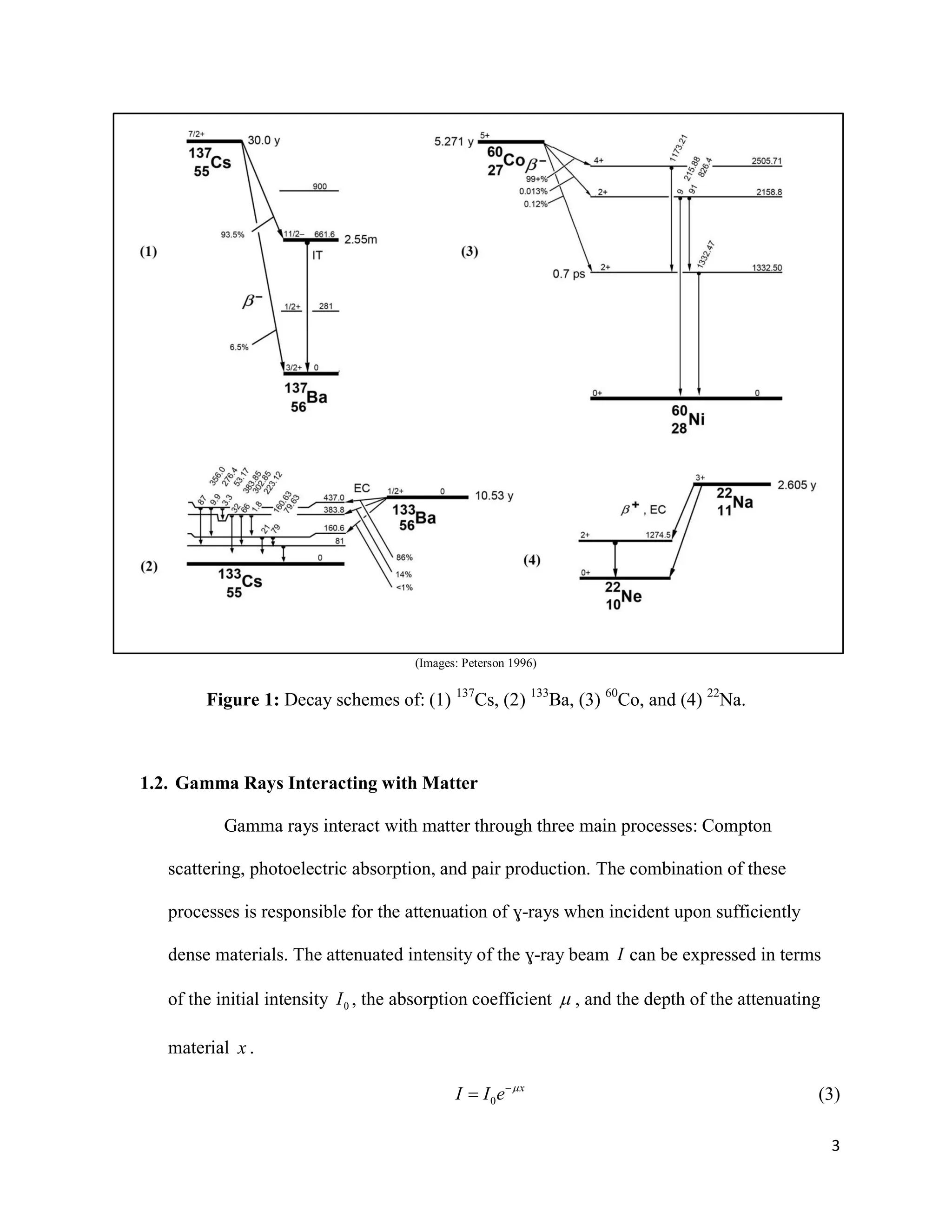
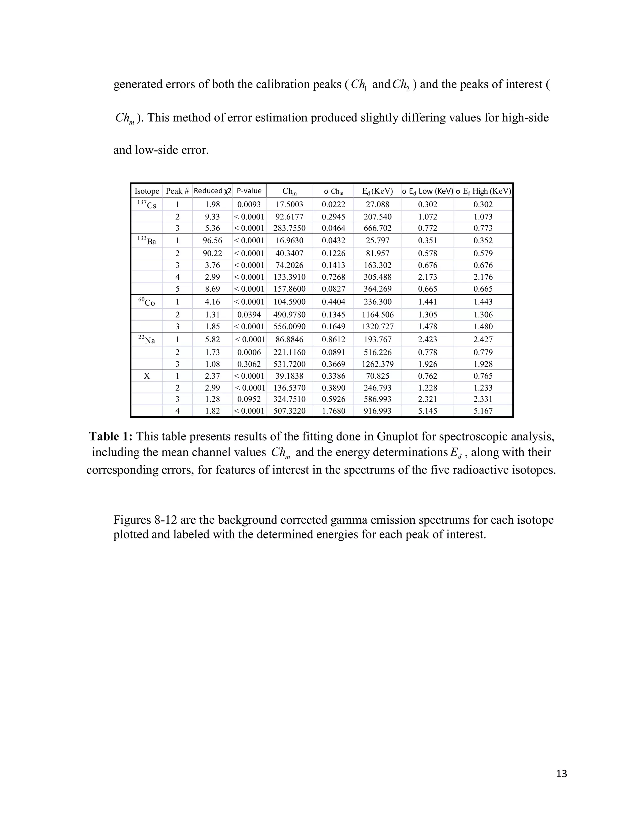
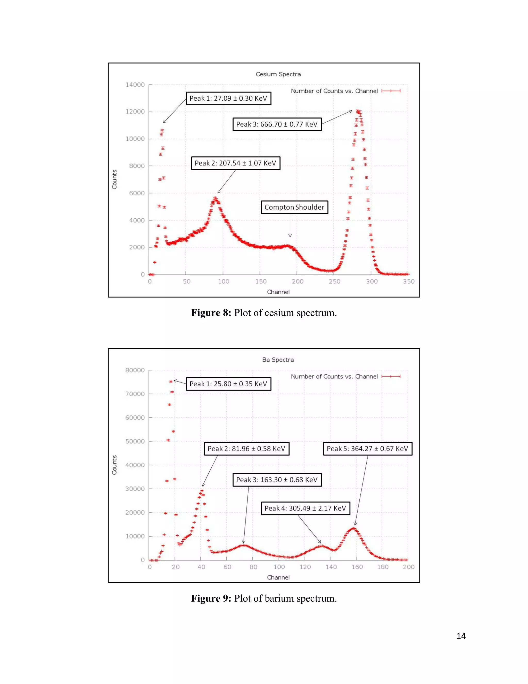
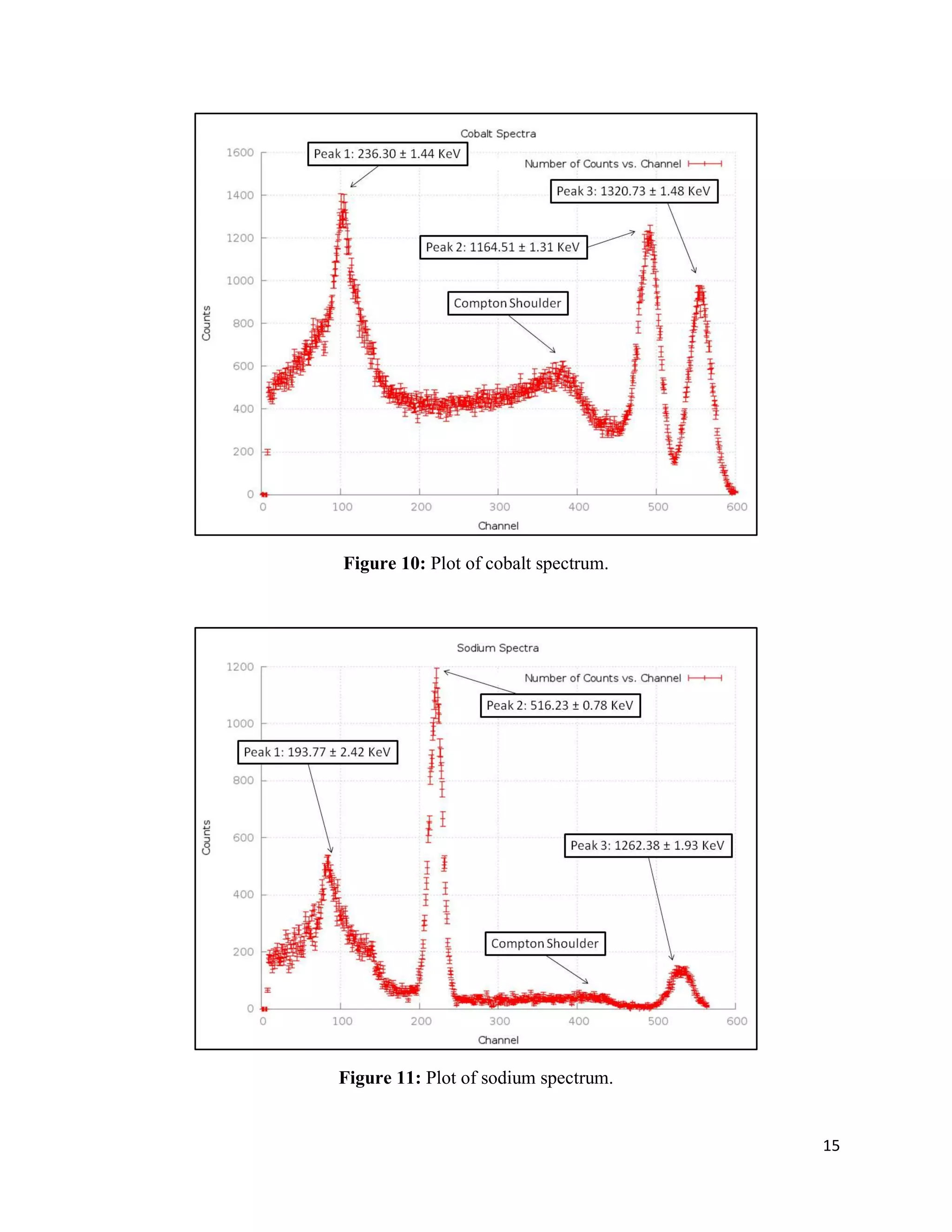
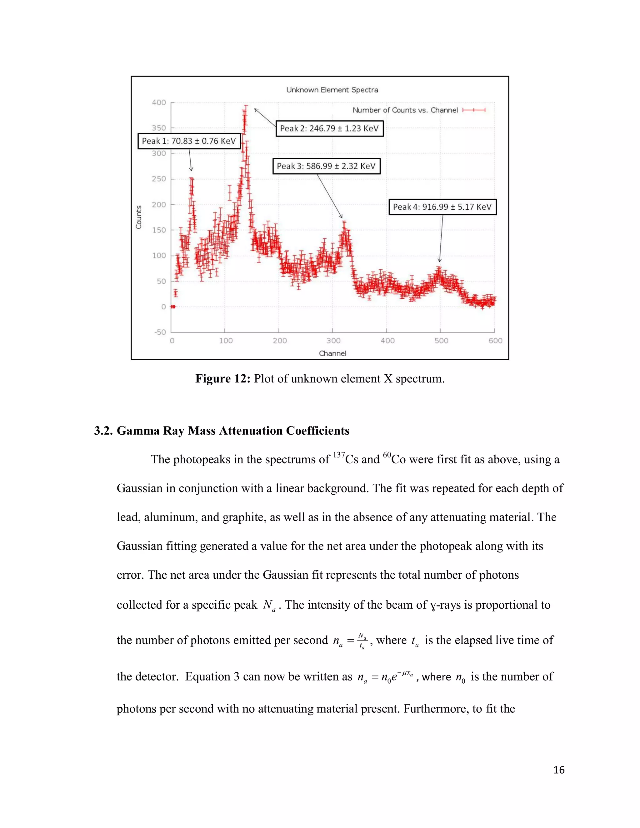
1) Gamma ray emission spectra were collected for isotopes 22Na, 60Co, 137Cs, and 133Ba and a mystery isotope was identified as 232Th.
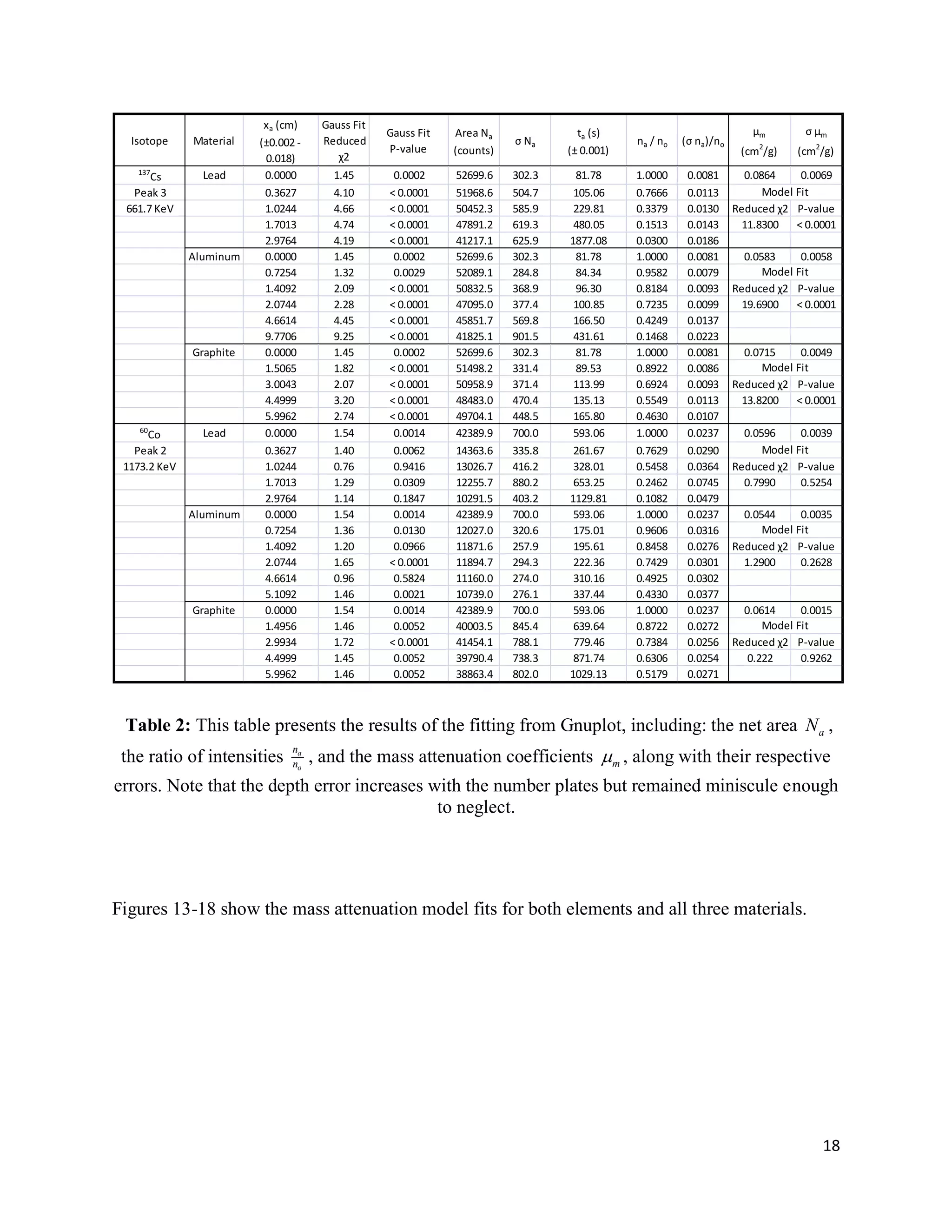
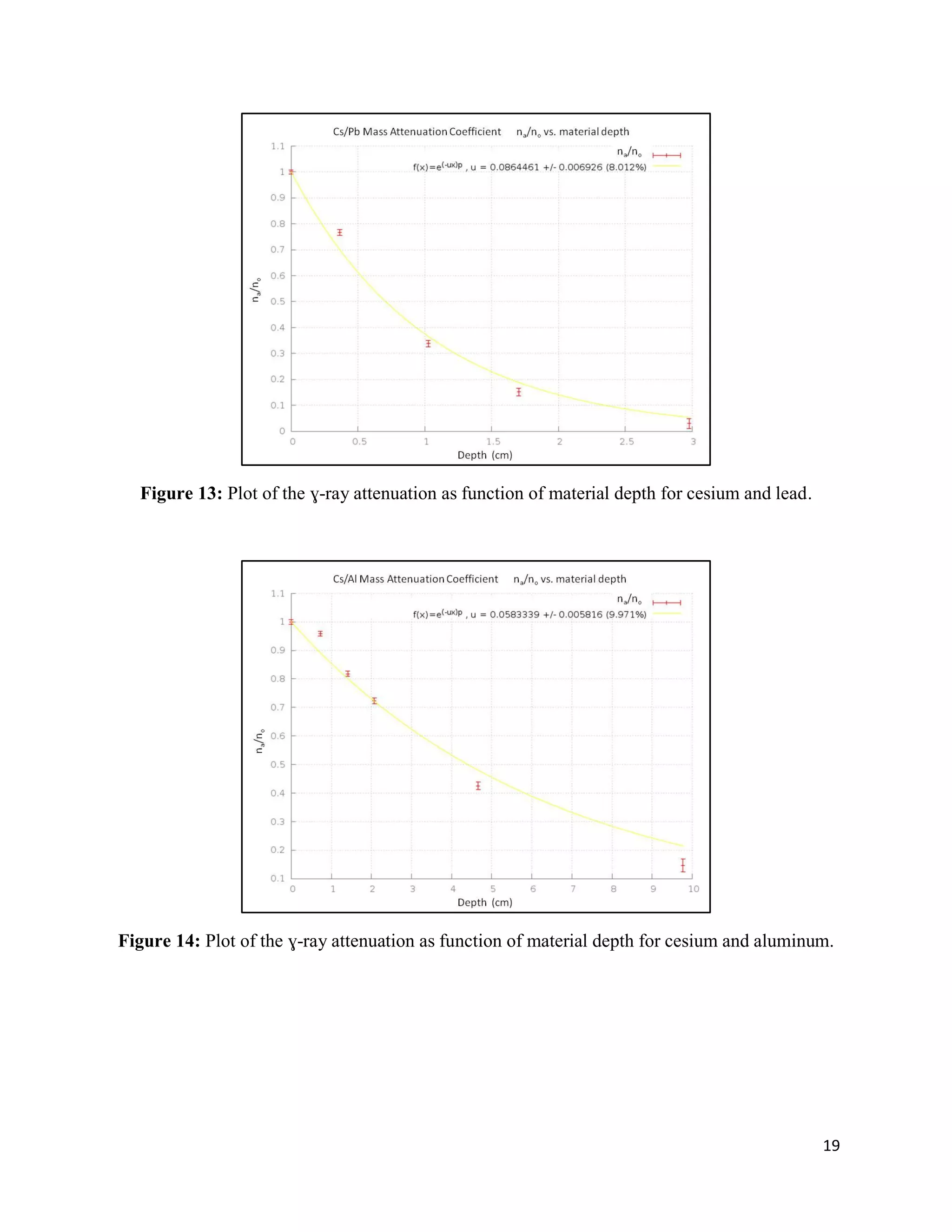
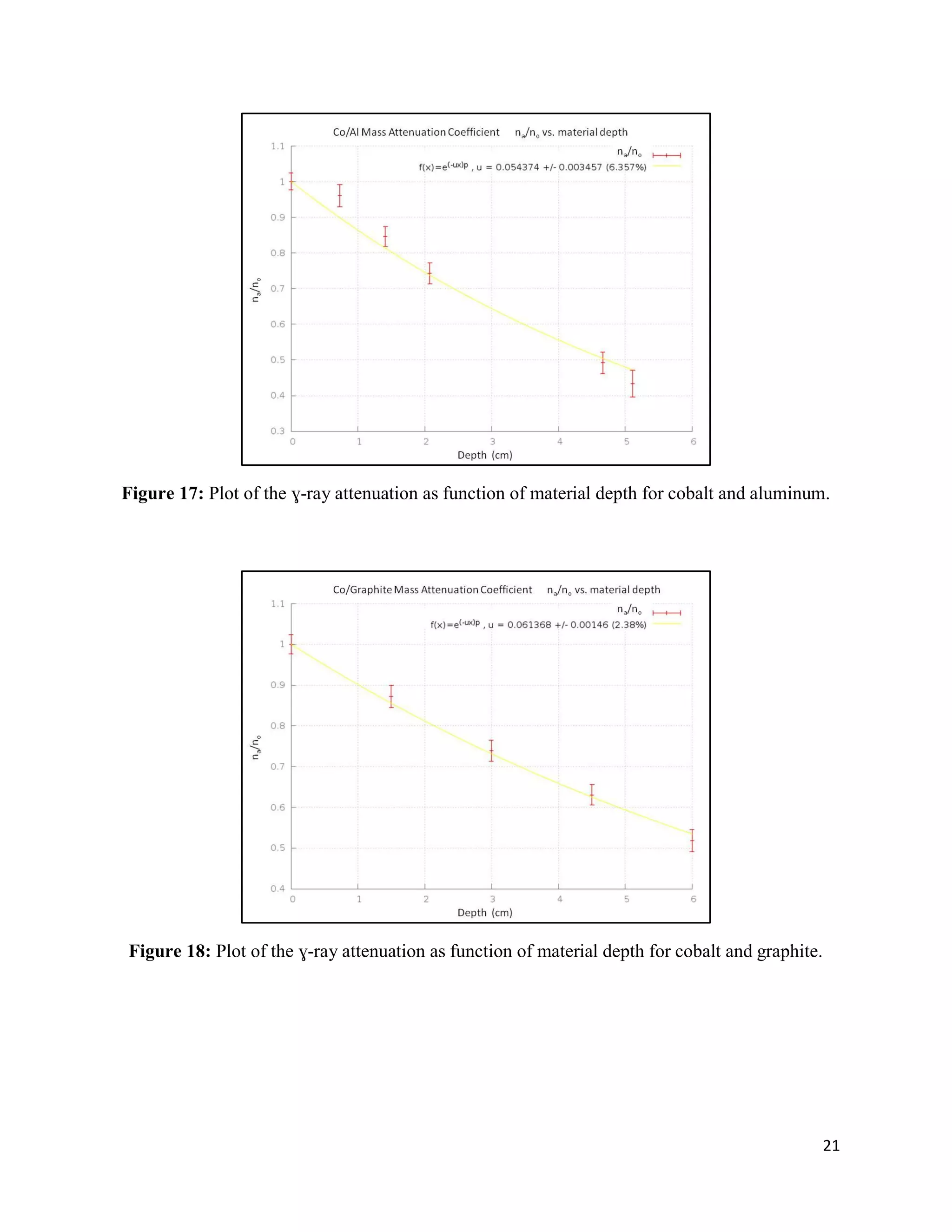
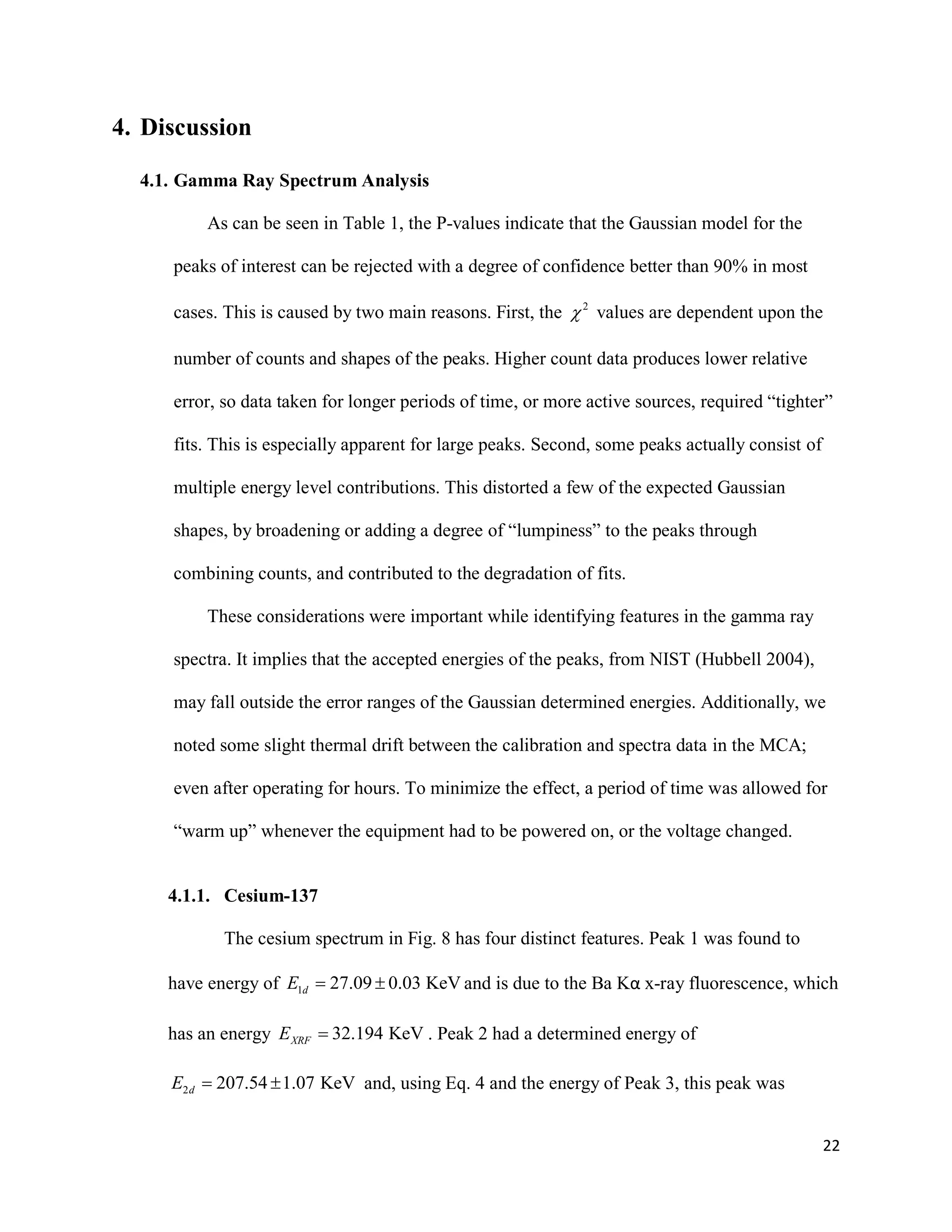
2) Exponential attenuation models were tested for 137Cs and 60Co interacting with lead, aluminum, and graphite. The model was rejected for 137Cs but not for 60Co.
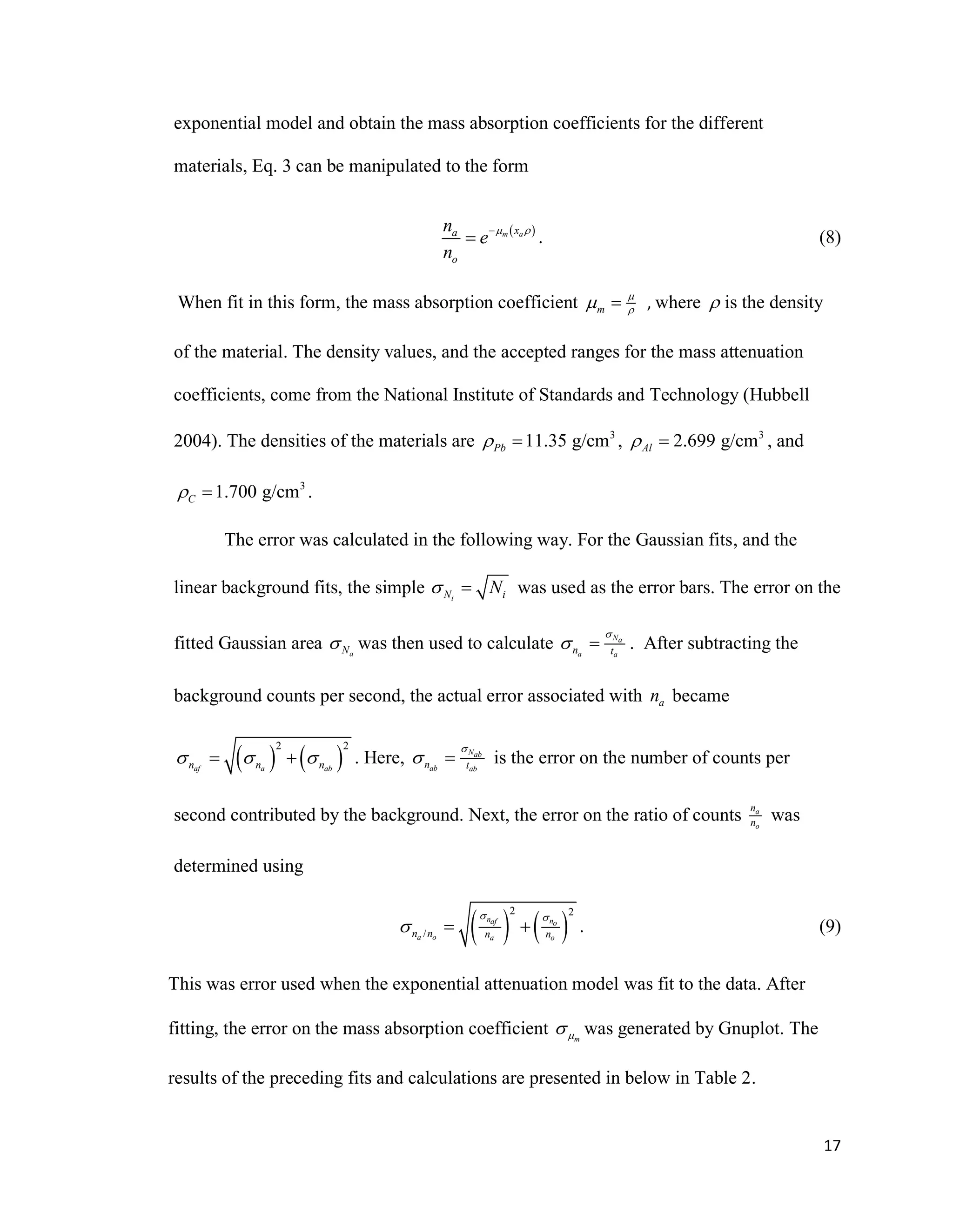
3) Mass attenuation coefficients were determined for the absorbing materials using photopeak photometry data from 137Cs and 60Co.