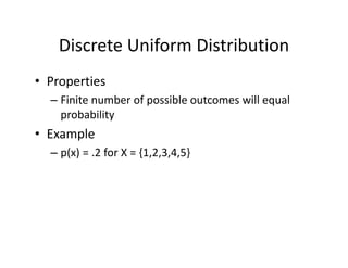
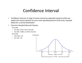
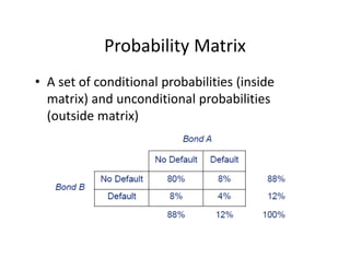
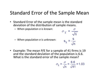
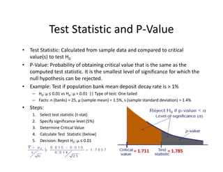
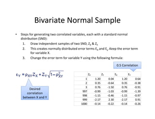
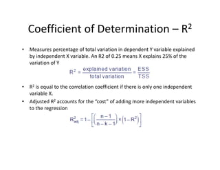
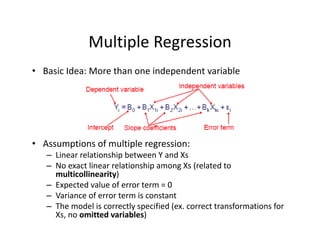
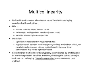
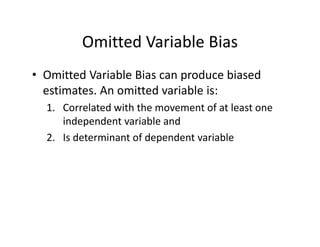
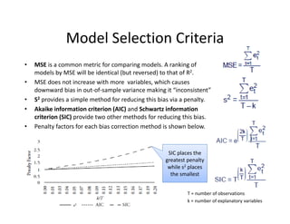
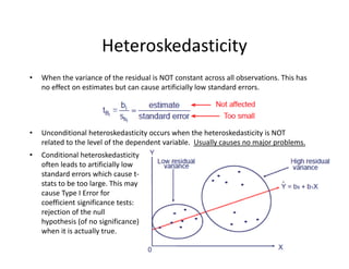
1) The document introduces several key concepts in probability theory and statistics including probability functions, distributions, measures of central tendency and dispersion.
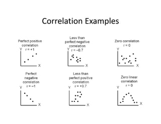
2) It covers topics such as probability, random variables, expectations, variance, covariance, correlation, and common distributions including the normal, binomial, and Poisson.
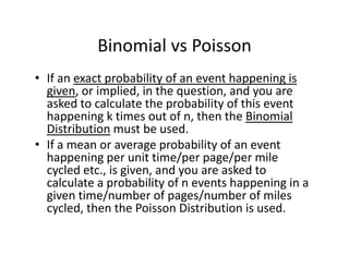
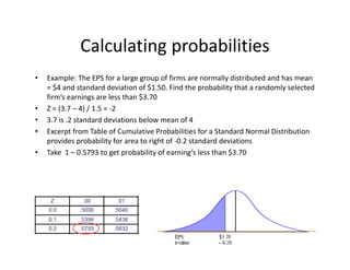
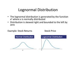
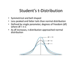
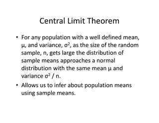
3) Examples are provided to help explain concepts like the difference between binomial and Poisson distributions and how the central limit theorem applies to sample means.
![Variance and Standard Deviation
• Variance = σ2 = E[(X – E(X))2], properties:
1. If c is constant: Var(c) = 0 and VaR(cX)=c2 x Var(X)
2. If c and a are constants: Var(aX+c ) = a2 x Var(X)
3. If c and a are constants: E(cX+a) = cE(X)+a
4. If X and Y are independent random variables:
Var(X+Y) = Var(X‐Y) = Var(X) + Var(Y)
• Standard Deviation = Square root of Variance
= σ = {E[(X – E(X))2]}1/2](https://image.slidesharecdn.com/6a7a5b80-4aac-4dda-ada0-970375a962a1-160726160328/85/FRM-Level-1-Part-2-Quantitative-Methods-including-Probability-Theory-10-320.jpg)
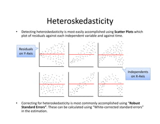
![Covariance
• Covariance: A measure of how to variables move together.
Cov(X,Y) = E[(X‐E(X))(Y‐E(Y))] = E(XY)‐E(X)E(Y)
• Interpretation:
– Values range from negative to positive infinity.
– Positive (negative) covariance means when one variable has
been above its mean the other variable has been above (below)
its mean.
– Units of covariance are difficult to interpret which is why we
more commonly use correlation (next slide)
• Properties:
– If X and Y are independent then Cov(X,Y) = 0
– Covariance of a variable X with itself is Var(X)
– If X and Y are NOT independent:
• Var(X+Y) = Var(X) + Var(Y) + 2(Cov(X,Y)
• Var(X‐Y) = Var(X) + Var(Y) ‐ 2(Cov(X,Y)](https://image.slidesharecdn.com/6a7a5b80-4aac-4dda-ada0-970375a962a1-160726160328/85/FRM-Level-1-Part-2-Quantitative-Methods-including-Probability-Theory-12-320.jpg)
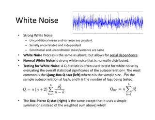
![• An F‐test is any statistical test in which the test statistic has an F‐distribution under the null
hypothesis.
• Often used to determine the best of two statistical models by identifying the one that best
fits the data they were both estimated upon.
• Tests whether any independent variables explain variation in dependent variable.
F‐statistic with k and n – (k+1) degrees of freedom
• k = number of independent variables (attributable to ESS)
• n – (k+1) = observations minus number of coefficients
Example:
• The ESS and SSR from a model are 500 and 200 respectivly
• Sample observations = 100, Model has 3 variables
• F = (500 / 3) / [200 /(100‐3‐1)] = 80
• Critical 95% F‐Value for 3 and 96 df = 2.72
F‐Test
Numerator Degrees
of Freedom
Denominator Degrees
of Freedom](https://image.slidesharecdn.com/6a7a5b80-4aac-4dda-ada0-970375a962a1-160726160328/85/FRM-Level-1-Part-2-Quantitative-Methods-including-Probability-Theory-44-320.jpg)
![Factor Models
• Factor models can be used to define correlations between normally distributed
variables.
• Equation below is for a one‐factor model where each Ui has a component
dependent on one common factor F in addition to another idiosyncratic factor Zi
that is uncorrelated with other variables.
• Steps to construct:
1. Create the SND common factor F
2. Choose a weight α for each Ui
3. Create correlations with F (previous slide)
4. Draw i number of SND idiosyncratic factors Z
5. Calculate U using equation to right
• Advantages of Single Factor Models:
– Covariance matrix is positive‐semidefinite
– Number of correlation estimations is reduced to N from [Nx(N‐1)]/2
• Capital Asset Pricing Model (CAPM) is well known example of Single Factor Model
Common
Factor
Idiosyncratic
Factor](https://image.slidesharecdn.com/6a7a5b80-4aac-4dda-ada0-970375a962a1-160726160328/85/FRM-Level-1-Part-2-Quantitative-Methods-including-Probability-Theory-48-320.jpg)


![Inverse Transform Method
• Converts a random number u that is between 0 and 1 to a number from
the inverse of the cumulative distribution function (CDF)
• For discrete distributions, the unit interval [0,1] on the y‐axis (representing
the CDF) is split into segments based on the cumulative probabilities of
the discrete variables
• For example, cumulative probabilities of 40% 75% and 100% could
correspond to values 5, 20, and 40.](https://image.slidesharecdn.com/6a7a5b80-4aac-4dda-ada0-970375a962a1-160726160328/85/FRM-Level-1-Part-2-Quantitative-Methods-including-Probability-Theory-76-320.jpg)